Scene Changes Understanding Framework Based on Graph Convolutional Networks and Swin Transformer Blocks for Monitoring LCLU Using High-Resolution Remote Sensing Images

Abstract

High-resolution remote sensing images with rich land surface structure can provide data support for accurately understanding more detailed change information of land cover and land use (LCLU) at different times. In this study, we present a novel scene change understanding framework for remote sensing which includes scene classification and change detection. To enhance the feature representation of images in scene classification, a robust label semantic relation learning (LSRL) network based on EfficientNet is presented for scene classification. It consists of a semantic relation learning module based on graph convolutional networks and a joint expression learning framework based on similarity. Since the bi-temporal remote sensing image pairs include spectral information in both temporal and spatial dimensions, land cover and land use change monitoring can be improved by using the relationship between different spatial and temporal locations. Therefore, a change detection method based on swin transformer blocks (STB-CD) is presented to obtain contextual relationships between targets. The experimental results on the LEVIR-CD, NWPU-RESISC45, and AID datasets demonstrate the superiority of LSRL and STB-CD over other state-of-the-art methods.

1. Introduction

Remote sensing high-resolution (HR) imagery [1] is capable of providing richly detailed structures of the land surface, which has unique advantages for detecting changes of fine land cover and land use (LCLU), and can also mine semantic level information according to the geometrical structures and spatial patterns of ground objects. However, the changes of simple ground objects cannot directly reflect the changes of scene semantics in the area [2]. In Figure 1, the new construction of houses in residential areas is not directly equivalent to the semantic changes of residential areas, so there is also a semantic gap between the changes of ground objects and the changes of scene semantics. Fueled by a variety of practical applications in the remote sensing community, we intend to effectively describe the changes of scene semantics while obtaining the change of the ground object, i.e., scene change understanding.

Currently, there is very little theory and research on the subject of scene change understanding, only a few works based on different scene tasks. Ref. [2] investigated the changes in spatial equity of greenery around residents in Guangdong, Hong Kong, and Macao’s Greater Bay Area by studying time series of remote sensing images from 1997 to 2017. Ref. [3] presents an end-to-end scene change understanding framework that observes the variation between two time-points using different types of input images (i.e., depth, RGB, and point cloud images). Meanwhile, Ref. [4] proposed two challenging task types: scene change detection and semantic simultaneous localisation and mapping. It is crucial to investigate the environment and comprehend the position and nature of every thing in it for indoor robotic systems that must interact intimately with humans. A new framework [5] is proposed that detects and describes changes occurring in 3D scenes observed from multiple perspectives with natural language text. In this paper, our scene change understanding is mainly based on the following two processes: (i) Scene classification: the purpose of this process is to output the most similar semantic label to each image to distinguish different scene categories [6]. (ii) Change detection: this process discriminates the changes of areas or phenomena in the same geographical area at different times [7,8].

In general, compared with natural scenes, remote sensing scenes are more complex and face more difficulties in terms of classification and detection tasks, for example, small inter-class dissimilarity, large intraclass variations, and smaller and more separated objects. In particular, remote sensing systems are affected by the changes in the solar position and ground target geometry during image acquisition, which cause different types of brightness and shadows in the same scene area.

To overcome these problems, we propose a novel framework for scene change understanding based on bi-temporal remote sensing images. The following are the contributions of this work:

1

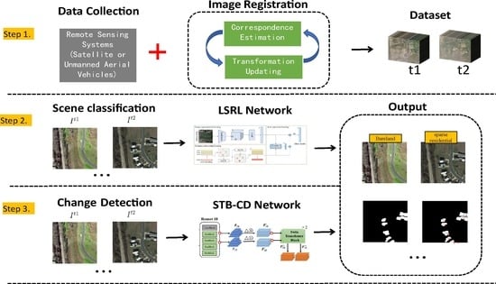
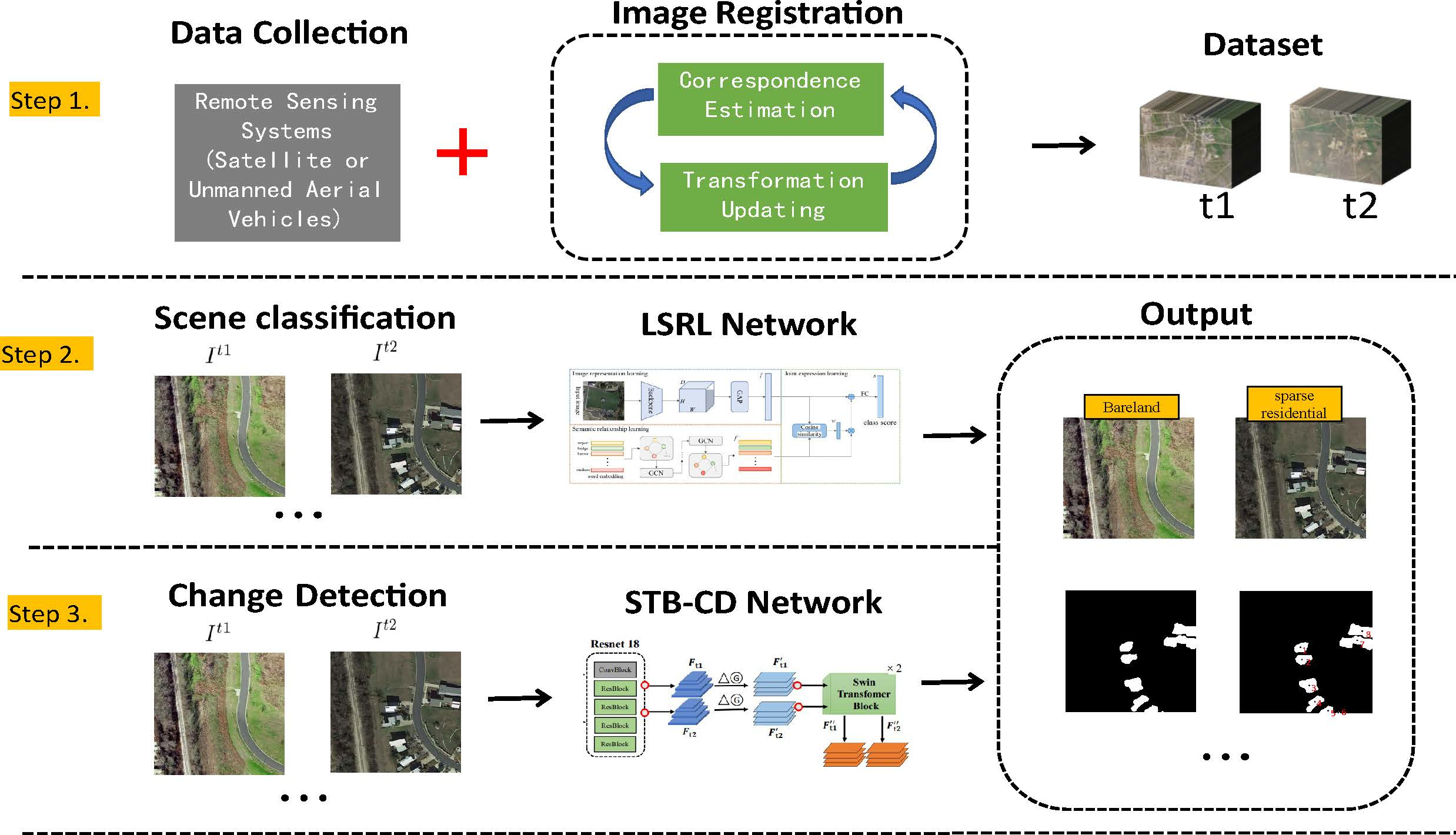
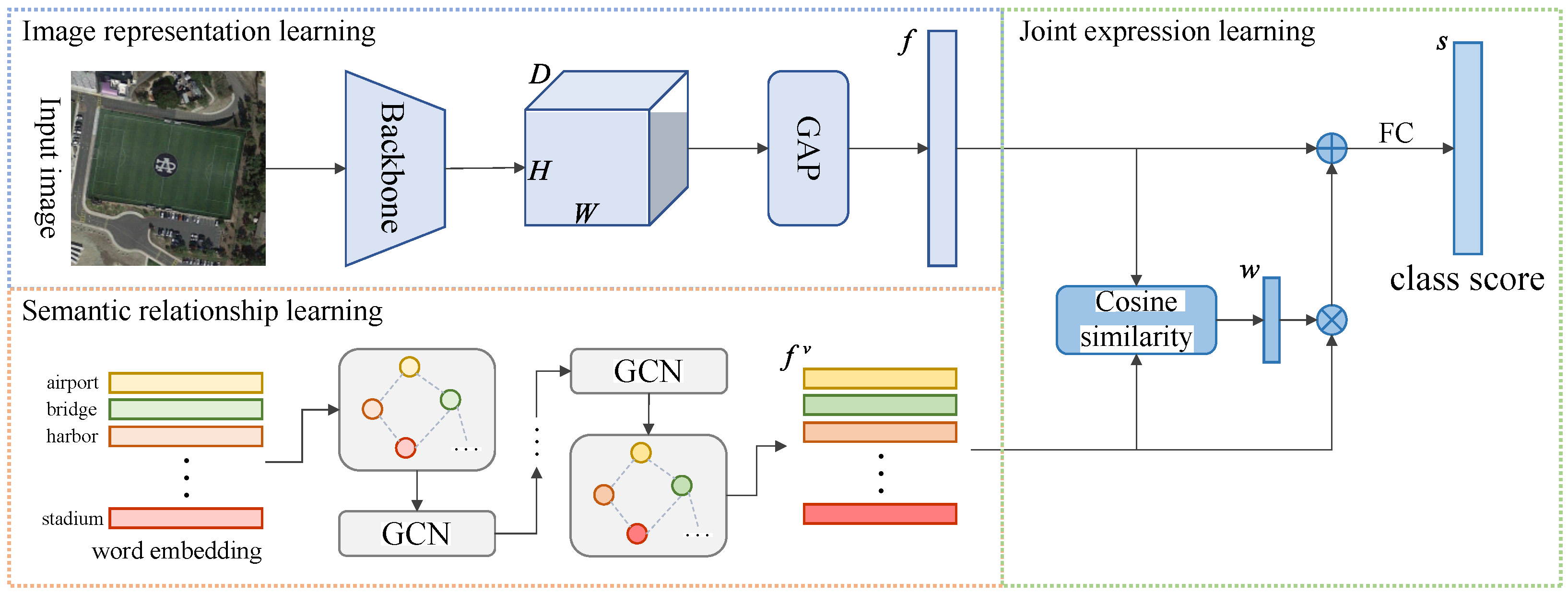
Based on EfficientNet, a robust LSRL network for scene classification is proposed. It consists of a semantic relation learning module based on graph convolutional networks and a joint expression learning framework based on similarity.

2

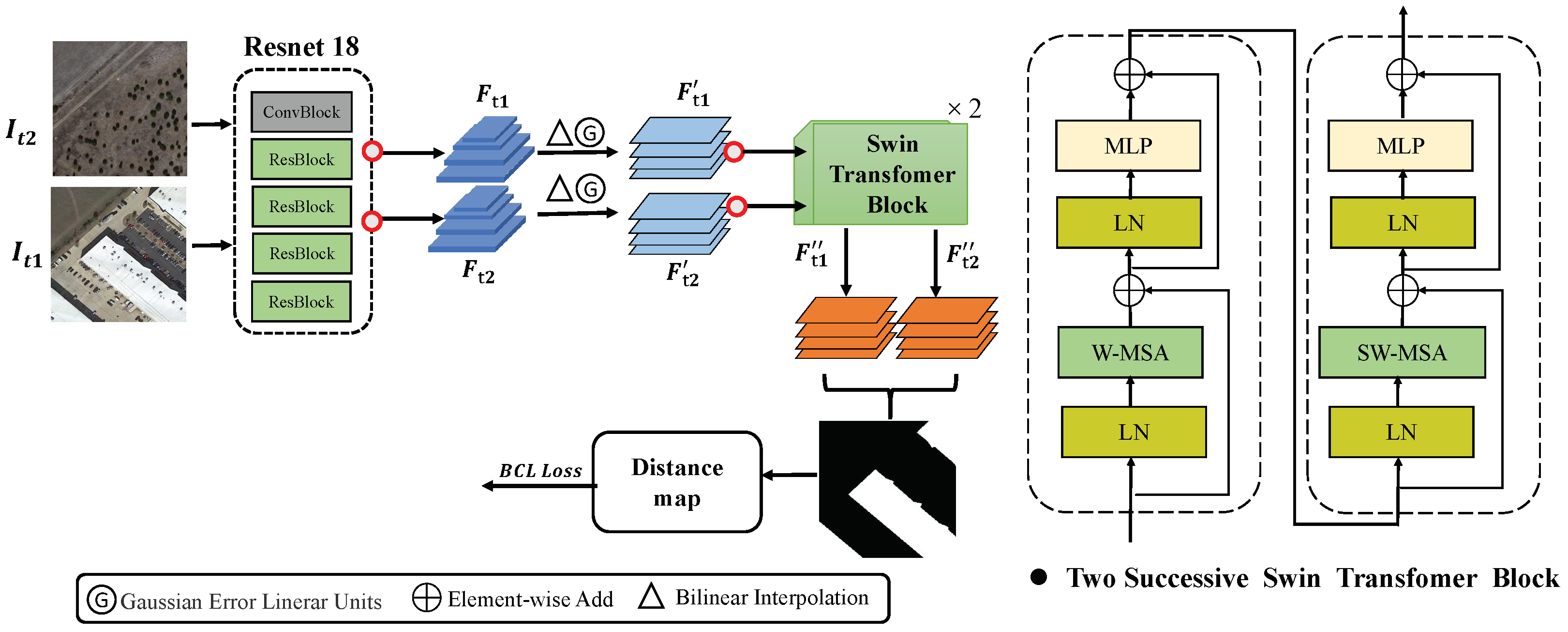
Simultaneously, we propose STB-CD for change detection on remote sensing images. STB-CD makes full use of the spatial and contextual relationships of the swin transformer blocks to identify areas of variation in buildings and green spaces of various scales.

3

The experiment results on the LEVIR-CD, NWPU-RESISC45, and AID datasets demonstrate the superiority of the two methods over state-of-the-art.

The rest of this paper is structured as follows. Section 1 is a description of related work. Section 2 describes the proposed framework for scene change understanding. Section 3 further describes the experimental details and results. Finally, the paper is summarized in Section 4.

2. Related Works

Our work builds on prior work in two domains: scene classification and change detection.

2.1. Scene Classification on Remote Sensing Images

Scene classification aims to accurately identify the high-level semantic labels to which different scenes belong according to their content. In recent decades, many studies have been conducted in military and civilian applications. Remote sensing scene classification relies heavily on the ability to efficiently and swiftly extract additional discriminative feature representations. Past methods mainly use manually designed feature descriptors, such as colour histograms [9], scale-invariant feature transform [10], and directional gradient histograms [11], to obtain the features representation of images. However, these methods rely heavily on the quality of the feature design and are unable to communicate high-level semantic data. As deep learning evolves, more and more models based on convolutional neural networks [6,12] have been used for scene classification, and by designing a series of network structures, the classification accuracy can be effectively improved. However, due to the increasing resolution of remote sensing images, the scenes contain more feature information and more complex spatial distribution, and the interclass similarity and intraclass diversity among different scenes increases the difficulty of scene classification. Therefore, to examine deconvolution networks for remote sensing scene classification, Ref. [6] proposed an unsupervised representation learning approach.

2.2. Change Detection on Remote Sensing Images

During the last few decades, many change detection methods have been proposed for gathering data on land cover change. Most methods in remote sensing rely on the difference between intensity. Ref. [13] proposed deep change vector analysis (DCVA) to generate robust feature vectors to model the spatial background information of remote sensing images. Lv et al. designed an object-oriented calculation of key point distances to measure the degree of variation between remote sensing images [14]. In order to generate difference images with a good separability for remote sensing images, Ref. [7] adopted a Fuzzy C-Means classifier to generate a similarity matrix between image a pair of geometric corrections. Ref. [15] presented three different types of fully convolutional neural networks (FC-Siam-conc, FC-Siam-diff, and FC-early fusion), which contain two skip-connection methods (connection and difference) and a pair of co-registered images. Deep learning-based algorithms are particularly suitable for effectively discriminating between real and complex irrelevant changes because these algorithms are robust (i.e., invariant) against differences in viewpoints and illumination conditions. However, these approaches still fail when dealing with targets of widely varying shape, size, and position in remotely sensed images. Therefore, some works fusing attention mechanisms (e.g., spatial attention, self-attention) to simulate the semantic connections between image pairings, such as the deep supervised attention metric network (DSAMNet) [16], have shown robustness and accuracy in promising results have been achieved.

3. Methodology

This section describes a robust scene change understanding framework using dual spatiotemporal remote sensing images. It has two main components: scene classification method (LSRL) and change detection method (STB-CD). The proposed framework is summarized in the latter part of this section.

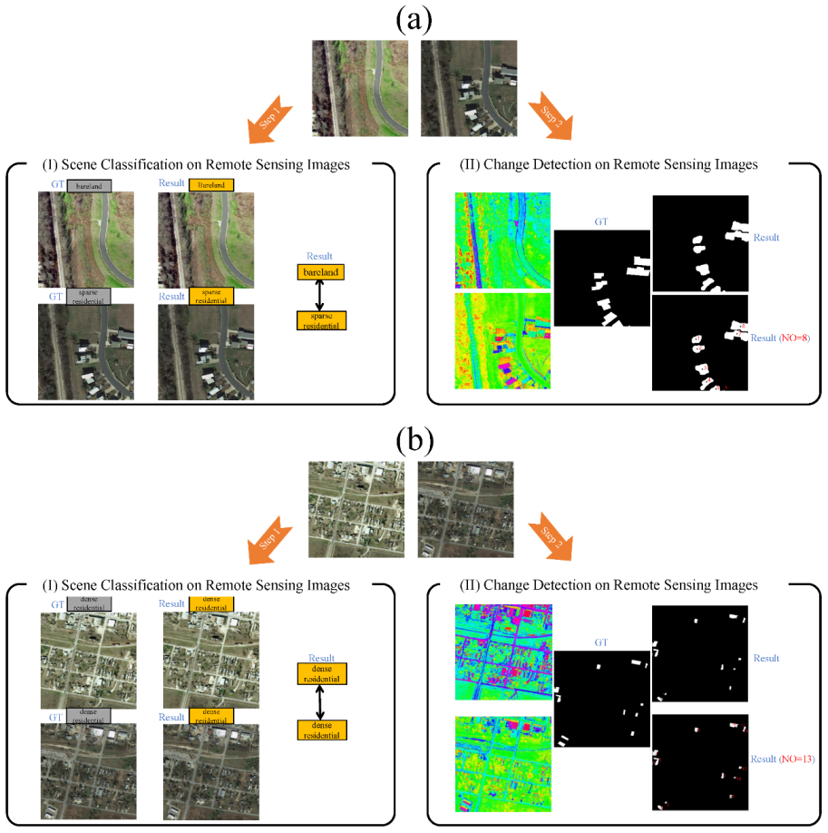
3.1. Scene Classification of Remote Sensing Images

How to effectively learn the semantic relations between labels of remote sensing scene categories to obtain more discriminative scene features is crucial for accurate classification. In this section, we detail the proposed label semantic relation learning (LSRL) network, which consists of a semantic relation learning module based on graph convolutional networks and a joint expression learning framework based on similarity. The overall framework model is shown in Figure 2.

Image representation learning. As an efficient convolutional neural network, efficientNet has achieved outstanding results in image classification. We directly apply this model as our backbone network. Specifically, given a remote sensing image, we use efficientNet to extract a feature map of size $W\times H\times D$. Then, a global level pooling (GAP) is applied to obtain the D-dimensional image features $f\in R^D$.

Semantic relationship learning. To learn semantic relations between category labels, we use graph structures to model the association between labels. For the learning process, the input data is defined as a graph $G=〈V,A〉$, where the graph nodes $V={\left\{v_i\right\}}_{i=1}^C$ are represented as $d_e\in R^C$ dimensional word embeddings of the category labels corresponding to the C scene categories. The adjacency matrix A describes the potential semantic relationships between different scene categories, and the operation can be written as

$$A_{ij}=\left\{\begin{array}{cc}1,& if\exists \widehat{ij}\\ 0,& otherwise\end{array}\right.$$

(1)

where $\widehat{ij}$ denotes the existence of a semantic relationship between category i and category j. In our experiments, the adjacency matrix A is predefined for different datasets. Then, we learn to convey information about the potential semantic relationships between different categories with the help of graph convolutional networks (GCN). For the $l+1$-layer GCN, both the node features $H^{\left(l\right)}$ of the previous layer and the adjacency matrix A are taken as input, and new node information is generated $H^{\left(l+1\right)}$. The node features at $l=0$ are initialized by the word embeddings of the input. Thus, the basic cyclic process can be formulated as

$$H^{\left(0\right)}=v{H}^{\left(l+1\right)}=\sigma \left(A{H}^{\left(l\right)}{W}^{\left(l\right)}\right)$$

(2)

where $W^{\left(l\right)}$ is the matrix of learnable weights for each layer, $\sigma \left(·\right)$ represents the nonlinear function. Eventually, the learned category label features are represented as $f^v=GCN\left(v,A\right)$.

Joint expression learning. Instead of the simple summation operation, we propose a cosine similarity-based joint expression learning framework. Specifically, the similarity coefficients $w_i$ of image features f and each category label feature $f_i^v\in R^D$ are first computed to obtain the coefficient vector w by

$$w={\left\{w_i=\frac{dot\left(f,f_i^v\right)}{{∥f∥}_2·{∥f_i^v∥}_2}\right\}}_{i=1}^C$$

(3)

where $dot\left(·\right)$ is the vector dot product, ${∥·∥}_2$ denoted as vector two-parametric operation. Then, in order to reduce the number of operations and avoid the interference of redundant features, we keep only the top k ($k=4$) large similarity coefficients and set the rest to 0. Based on the different similarity coefficients, the category label vectors are fused into the image features, which can be expressed as

$$f^{\prime }=f+\sum _{i=1}^C{w}_i{f}_i^v$$

(4)

A simple fully connected layer is finally used to the feature vector to compute the classification score vector s of the input image.

3.2. Change Detection on Remote Sensing Images

Three components make up the proposed network (STB-CD): multiscale feature extraction learning, spatial relations learning, and a new loss function. To extract distinctive features of all scale ground objects, multiscale features are extracted automatically from bi-temporal inputs by the feature extractor. Subsequently, spatial relations learning is constructed for improving the global and local relationship between the ground objects. Moreover, the losses for optimization are calculated by comparison with the ground truth. Figure 3 illustrates the overall flow of our STB-CD.

Multiscale feature extraction learning. The image pair ${\widehat{I}}_{t1}$ and ${\widehat{I}}_{t2}$ is input to ResNet18 to extract features, and all obtain a set of multi-scale features $F_t$ ($f_1$, $f_2$, $f_3$ and $f_4$), $t=t1,t2$.

Spatial and temporal relations learning. Since the bi–temporal remote sensing image pair is composed of spatial spectral information and temporal spectral information, the performance of the CD method can be improved by using the relationship between them. First, multiscale features $F_{t1}^{{}^{\prime }}$ and $F_{t2}^{{}^{\prime }}$ are partitioned into non-overlapping patches, and we view each patch as a “token”. Subsequently, a linear input layer for each feature sends it to any dimension (expressed as C). Meanwhile, the method applies swin transformer to the tokens independently, which are made up of a shifted-window-mechanism-based multi-head local self attention ((S)W-MSA) and multi-layer perceptron blocks. The strength of (S)W-MSA is that it can be concerned with inputs for several windows at different spatial locations at the same time. We divide the feature map $f^{{}^{\prime }}$ uniformly into $7\times 7$ windows. Therefore, the attention matrix is calculated by self-attention mechanism in each window, which is expressed as:

$$\begin{array}{c}\hfill Att(Q,K,V)=\sigma (\frac{Q{K}^T}{\sqrt{d}}+B)V\end{array}$$

(5)

where $\sigma (·)$ and $B\in {\Re }^{p^2\times p^2}$ are a nonlinear function and a learnable deviation [17], respectively. Generally, $Q,K,V\in {\Re }^{p^2\times d}$ are the attention information, $\sqrt{d}$ and $p^2$ denote the channel dimension and the number of patches, respectively.

Thereafter, we resize the two features $F_t^{{}^{″}}(m=t1,t2)$ to the equivalent size of the incoming image through bilinear interpolation and compute the euclidean distance $Dist$ between the features, according to the following formula:

$$Dist=\sqrt{(F_{t1}^{{}^{″}}-F_{t2}^{{}^{″}})\times {(F_{t1}^{{}^{″}}-F_{t2}^{{}^{″}})}^T}$$

(6)

where $F_{t1}^{{}^{″}}$ and $F_{t2}^{{}^{″}}$ denote the resized feature map of $t1$ and $t2$, respectively.

Loss function. To create the contrast loss required for optimization, $Dist$ is compared to the ground truth during training. Suppose that ${\widehat{I}}_{t_1}^b$$\in {\Re }^{B\times 3\times H\times W}$ and ${\widehat{I}}_{t_2}^b$$\in {\Re }^{B\times 3\times H\times W}$ are regarded as a batch bi_temporal image pairs ($M^{gt}$, $M^p$), where $M^{gt}$ denotes a set of Ground Truth binary label mappings, $M^p$ is generated using our model. Considering the positive–negative label imbalance of our samples at the beginning of training, the loss function is defined as

$$\begin{array}{c}\hfill L_{bcl}(M^p,M^{gt})=\frac{1}{2}\frac{1}{N_c}\sum _{b,h,w}{M}_{b,h,w}^{gt}Max(0,m-M_{b,h,w}^p)\\ \hfill +\frac{1}{2}\frac{1}{N_{uc}}\sum _{b,h,w}(1-M_{b,h,w}^{gt})M_{b,h,w}^p\end{array}$$

(7)

where $b,1\le b\le B$ denote the index of B, $w,h$ are width and height of image, 0 and 1 indicate unchanged and changed state. Pairs of changing pixels with distance greater than $m(m=2)$ have no effect on the loss function. $N_{uc}$ and $N_c$ represent the quantity of unchanged and changed pixel pairs, calculated as:

$$N_{uc}=\sum _{b,h,w}(1-M_{b,h,w}^{gt})$$

(8)

$$N_c=\sum _{b,h,w}{M}_{b,h,w}^{gt}$$

(9)

4. Experiments

In this subsection, we experimentally verify the feasibility of our proposed framework. We will begin with our experimental settings and then present the implmentation details and benchmark the state-of-the-art models. Finally, we present a detailed performance analysis.

4.1. Datasets

In our experiments, in order to achieve the theoretical goal of scene change understanding and simultaneously examine the feasibility of the proposed scene classification and change detection methods, we selected change detection and scene classification datasets with similar ground objects and resolutions, and carried out validation experiments (Algorithm 1).

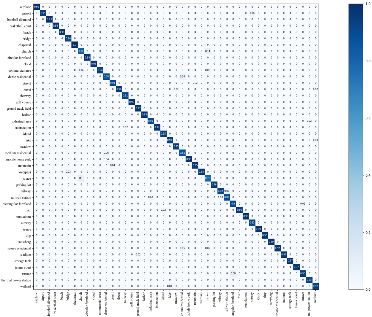
• NWPU-RESISC45 dataset [18] is the most widely used benchmark for remote sensing scene classification at the moment. It is made up of 31,500 images, covering 45 scene categories: mountain, runway, sea ice, ship, stadium, airplane, desert, circular farmland, basketball court, forest, meadow, airport, baseball diamond, bridge, beach, mobile home park, overpass, palace, river, roundabout, snow berg, harbor, storage tank, church, cloud, lake, commercial area, railway, intersection, railway station, industrial area, rectangular farmland, tennis court, chaparral, dense residential, freeway, sparse residential, terrace, thermal power station, island, wetland, golf course, ground track field, and medium residential. There are 700 images in each category, each having a resolution of $256\times 256$ pixels. When conducting evaluation experiments, a wide range of training and test set ratios are used: 1:9 and 2:8.
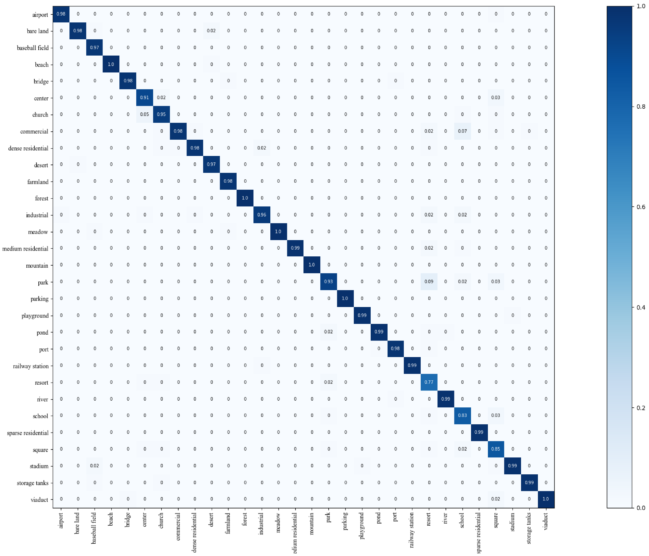
• Aerial Image Dataset (AID) [19] is a multi-source aerial scene classification dataset captured with different sensors. 10,000 photos of a $600\times 600$ pixel size are included, consisting of 30 scene categories, including mountain, park, desert, farmland, forest, industrial, river, school, sparse residential, square, airport, bare land, baseball field, railway station, resort, stadium, beach, bridge, center, church, parking, playground, pond, commercial, dense residential, meadow, port, storage tanks, viaduct, and medium residential. Each category has 220 to 420 images. When conducting evaluation experiments, a wide range of training and test set ratios are used: 2:8 and 5:5.
• LEVIR-CD [20] is a public large scale building change detection dataset, which contains 637 pairs of very high-resolution (0.5 m/pixel) remote sesing images of size $1024\times 1024$ pixels. LEVIR-CD includes different types of buildings, such as small garages, large warehouses, villa residences, and tall apartments. We follow its default dataset segmentation rules. In addition, the image is cut into $256\times 256$ small pieces without overlap. Finally, $7120/1024/2048$ patch pairs were obtained for training, validation, and testing, respectively.

Algorithm 1: Scene Changes Understanding Framework based on Graph Convolutional Networks and Swin Transformer Blocks for Monitoring LCLU using High-Resolution Remote Sensing Images.

Input: A pair of images of size $W\times H\times C$ taken at time $t1$ and $t2$, respectively. Output: Semantic changes and distance map $Dist$. ⊳Scene classification on remote sensing images (LSRL).   (i) Image representation learning:      extract a feature map of size $W\times H\times D$ via EfficientNet;      obtain the D-dimensional image features $f\in R^D$.   (ii) Semantic relationship learning:      compute the adjacency matrix A between different scene categories by Equation $\left(1\right)$;      learn to convey information about the potential semantic relationships between different categories using graph GCN.   (iii) Joint expression learning:      obtain the coefficient vector w by Equation $\left(3\right)$;      Then, to reduce the amount of operations and avoid the interference of redundant features, the category label vectors are calculated by Equation $\left(4\right)$. ⊳Change detection on remote sensing images (STB-CD).   (i) Multiscale feature extraction learning.      extract multiscale features $F_{t1}$ and $F_{t2}$ via ResNet 18;   (ii) Spatial relations learning:      compute a distance map D between reconstructed features $F_{t1}^{{}^{″}}$ and $F_{t2}^{{}^{″}}$ by Equation (6);   (iii) Loss function:      calculate loss of a batch bi_temporal images by Equations (7)–(9).

4.2. Evaluation Criteria

The F1 score, precision, recall, and IoU are applied to evaluate the improvement of our method. In addition, we employed the two most generally used quantitative assessment criteria in scene classification to assess the validity of the design approach, in terms of the confusion matrix (CM) and the overall accuracy (OA). The OA of the classification network is determined by dividing the number of successfully categorized pictures by the total number of images. This is a direct reflection of the overall effect of the network. The CM is calculated as the direct relationship between the true and predicted labels of each category. The confusion matrix focuses on analyzing the misclassification of each category to assess the robustness of the model. The corresponding equations are as follows:

$$F_1=\frac{2}{{Precision}^{-1}+{Recall}^{-1}}$$

(10)

$$Precision=\frac{TP}{TP+FP}$$

(11)

$$Recall=\frac{TP}{TP+FN}$$

(12)

where $TP$, $FP$, and $TP+FN$ denote the number of true positives, the false positives, and all ground truths, respectively.

4.3. Implementation Details

LSRL and STB-CD were implemented using PyTorch library. As for the LSRL, the optimizer adopts stochastic gradient descent (SGD), momentum set to 0.9. 30 training epochs and 8 batch sizes are used. The learning rate was initially set at 0.01. Moreover, to make the experimental outcomes more reliable, we repeat the training ten times with the identical parameter values. Then we compute the mean value and standard deviation. As for the STB-CD, we use Adam solver as the optimizer with an initial learning rate of 0.0001 on LEVIR-CD dataset, and a batch size of 4 sample pars was adopted to train the model. All of our experiments were conducted on a workstation consisting of an Nvidia GeForce Titan Xp GPU with 12 GB of video memory and an Intel(R) Core(TM) i7-7700K CPU with 32 GB of memory.

4.4. Comparisons of Scene Classification

Eight cutting-edge scene classification techniques are put up against the suggested LSRL approach in this comparison: MDFR (Multi-scale Deep Feature Representation) [21], VGG19 [22], SAFF (Self-attention-based Deep Feature Fusion) [23], EfficientNetB3-Attn-2 [24], H-GCN (High-order Graph Convolutional Network) [25], DMA (Dual-Model Architecture) [12], SEMSDNet (Multiscale Dense Networks with Squeeze and Excitation Attention) [26], and LCNN-CMGF (Lightweight Convolutional Neural Network based on Channel Multi-Group Fusion) [27]. For the AID dataset, as shown in

Table 1. The OA(%) of different methods on AID dataset.

Methods	20% Training Ratio	50% Training Ratio
MDFR [21]	90.62 ± 0.27	93.37 ± 0.29
VGG19 [22]	87.73 ± 0.25	91.71 ± 0.24
SAFF [23]	90.25 ± 0.29	93.83 ± 0.28
EfficientNetB3-Attn-2 [24]	92.48 ± 0.76	95.39 ± 0.43
H-GCN [25]	93.06 ± 0.26	95.78 ± 0.37
DMA [12]	94.05 ± 0.10	96.12 ± 0.14
LSRL (ours)	96.44 ± 0.10	97.36 ± 0.21

, LSRL achieves 96.44% and 97.36% overall accuracy at 20% and 50% training ratios, respectively, showing the best classification performance. For NWPU-RESISC45, the complete experimental results are shown in

Table 2. The OA(%) of different methods on NWPU-RESISC45 dataset.

Methods	10% Training Ratio	20% Training Ratio
MDFR [21]	83.37 ± 0.26	86.89 ± 0.17
VGG19 [22]	81.34 ± 0.32	83.57 ± 0.37
SAFF [23]	84.38 ± 0.19	87.86 ± 0.14
H-GCN [25]	91.39 ± 0.19	93.62 ± 0.28
SEMSDNet [26]	91.68 ± 0.39	93.89 ± 0.63
LCNN-CMGF [27]	92.53 ± 0.56	94.18 ± 0.35
LSRL (ours)	93.45 ± 0.16	94.27 ± 0.44

, where our method achieves an overall accuracy of 94.27% when the training ratio is 20%. A training ratio of 10% achieves an OA of 93.45%, and both are superior to the other approaches.

In addition, Figure 4 and Figure 5 show the confusion matrices in the AID when the training ratio is 20% and in the NWPU-RESISC45 dataset when the training ratio is 20%, respectively. In NWPU-RESISC45, the categories of palace and church produce greater confusion, with 10% of the palaces being misclassified as churches. The possible reason for the analysis is that because we designed the adjacency matrix to associate the palace and church classes and considered them to have a strong semantic relationship. However, all other classes achieved high classification accuracy and proved the effectiveness of the proposed method.

4.5. Comparisons of Change Detection

On the LEVIR-CD dataset, we contrast the efficiency of our proposed change detection method (STB-CD) with that of four cutting-edge approaches: FC-EF [15], FC-Siam-diff [15], FC-Siam-conc [15], and STANet (Spatial–temporal Attention Neural Network) [20]. FC-Siam-diff and FC-Siam-conc are an extension of FC-EF. Experimental comparison results of all methods are listed in

Table 3. Experimental Results on LEVIR-CD Dataset.

Methods	Pre (%)	Rec (%)	F1 (%)	IOU (%)
FC-EF [15]	86.91	80.17	83.40	71.53
FC-Siam-diff [15]	89.53	83.31	86.31	75.92
FC-Siam-conc [15]	91.99	76.77	83.69	71.96
STANet [20]	83.81	91.00	87.26	77.40
STB-CD (ours)	86.51	88.27	87.38	77.60

. From the data in Table 3, the proposed method significantly outperformes other change detection methods, achieving the best performance (F1: $87.38\%$, IoU: $77.60\%$). The STANet yield obtains more integral change areas in most cases (F1 and IOU: $87.26\%$ and $77.40\%$). Moreover, FC-Siam-diff outperforms FC-EF and FC-Siam-diff, with 86.31% F1 and 75.92% IoU, respectively.

We visualize the experimental results of the proposed framework to demonstrate the entire execution flow of the proposed framework more intuitively. According to Figure 6, the proposed method achieved satisfactory results.

5. Conclusions

We have introduced a novel scene changes understanding framework for monitoring LCLU changes by applying HR remote sensing images, which consists of two steps: scene classification (LSRL) and change detection (STB-CD). LSRL adopts a semantic-relation-learning module based on graph convolutional networks and a joint-expression-learning-framework-based similarity. Meanwhile, STB-CD for change detection is introduced. It fully applies the spatial and context relationship of swin transformer blocks to detect changes in different buildings and green space areas. The results on the LEVIR-CD, NWPU-RESISC45, and AID datasets show the two designed methods have advantages over other state-of-the-art methods (Scene Classification Methods: MDFR, VGG19, SAFF, EfficientNetB3-Attn-2, H-GCN, DMA, SEMSDNet, and LCNN-CMGF; Change Detection Methods: FC-EF, FC-Siam-diff, FC-Siam-conc, and STANet). In our experiments, we mainly choose remote sensing images with a resolution of 0.5 m/pixel. In future work, we will carry out further related research on remote sensing images of different resolutions. In addition, we will conduct further research on scattered scenes and targets (e.g., aircraft) to meet the dynamic monitoring of different types of remote sensing scenes.

References

1. Zhang, X.; Xiao, P.; Feng, X.; Yuan, M. Separate segmentation of multi-temporal high-resolution remote sensing images for object-based change detection in urban area. Remote Sens. Environ. 2017, 201, 243–255. [Google Scholar] [CrossRef]
2. Yang, G.; Zhao, Y.; Xing, H.; Fu, Y.; Liu, G.; Kang, X.; Mai, X. Understanding the changes in spatial fairness of urban greenery using time-series remote sensing images: A case study of Guangdong-Hong Kong-Macao Greater Bay. Sci. Total Environ. 2020, 715, 136763. [Google Scholar] [CrossRef] [PubMed]
3. Qiu, Y.; Satoh, Y.; Suzuki, R.; Iwata, K.; Kataoka, H. Indoor scene change captioning based on multimodality data. Sensors 2020, 20, 4761. [Google Scholar] [CrossRef] [PubMed]
4. Qiu, Y.; Satoh, Y.; Suzuki, R.; Iwata, K.; Kataoka, H. 3d-aware scene change captioning from multiview images. IEEE Robot. Autom. Lett. 2020, 5, 4743–4750. [Google Scholar] [CrossRef]
5. Hall, D.; Talbot, B.; Bista, S.R.; Zhang, H.; Smith, R.; Dayoub, F.; Sünderhauf, N. The robotic vision scene understanding challenge. arXiv 2020, arXiv:2009.05246. [Google Scholar]
6. Lu, X.; Zheng, X.; Yuan, Y. Remote sensing scene classification by unsupervised representation learning. IEEE Trans. Geosci. Remote Sens. 2017, 55, 5148–5157. [Google Scholar] [CrossRef]
7. Song, F.; Yang, Z.; Gao, X.; Dan, T.; Yang, Y.; Zhao, W.; Yu, R. Multi-scale feature based land cover change detection in mountainous terrain using multi-temporal and multi-sensor remote sensing images. IEEE Access 2018, 6, 77494–77508. [Google Scholar] [CrossRef]
8. Song, F.; Zhang, S.; Lei, T.; Song, Y.; Peng, Z. MSTDSNet-CD: Multiscale Swin Transformer and Deeply Supervised Network for Change Detection of the Fast-Growing Urban Regions. IEEE Geosci. Remote Sens. Lett. 2022, 19, 6508505. [Google Scholar] [CrossRef]
9. Swain, M.J.; Ballard, D.H. Color indexing. Int. J. Comput. Vis. 1991, 7, 11–32. [Google Scholar] [CrossRef]
10. Lowe, D.G. Distinctive image features from scale-invariant keypoints. Int. J. Comput. Vis. 2004, 60, 91–110. [Google Scholar] [CrossRef]
11. Dalal, N.; Triggs, B. Histograms of oriented gradients for human detection. In Proceedings of the 2005 IEEE computer society conference on computer vision and pattern recognition (CVPR’05), San Diego, CA, USA, 20–25 June 2005; Volume 1, pp. 886–893. [Google Scholar]
12. Shen, J.; Zhang, T.; Wang, Y.; Wang, R.; Wang, Q.; Qi, M. A Dual-Model Architecture with Grouping-Attention-Fusion for Remote Sensing Scene Classification. Remote Sens. 2021, 13, 433. [Google Scholar] [CrossRef]
13. Saha, S.; Bovolo, F.; Bruzzone, L. Unsupervised deep change vector analysis for multiple-change detection in VHR images. IEEE Trans. Geosci. Remote Sens. 2019, 57, 3677–3693. [Google Scholar] [CrossRef]
14. Lv, Z.; Liu, T.; Benediktsson, J.A. Object-oriented key point vector distance for binary land cover change detection using VHR remote sensing images. IEEE Trans. Geosci. Remote Sens. 2020, 58, 6524–6533. [Google Scholar] [CrossRef]
15. Daudt, R.C.; Le Saux, B.; Boulch, A. Fully convolutional siamese networks for change detection. In Proceedings of the 2018 25th IEEE International Conference on Image Processing (ICIP), Athens, Greece, 7–10 October 2018; pp. 4063–4067. [Google Scholar]
16. Shi, Q.; Liu, M.; Li, S.; Liu, X.; Wang, F.; Zhang, L. A deeply supervised attention metric-Based network and an open aerial image dataset for remote sensing change detection. IEEE Trans. Geosci. Remote Sens. 2021, 60, 5604816. [Google Scholar] [CrossRef]
17. Liu, Z.; Lin, Y.; Cao, Y.; Hu, H.; Wei, Y.; Zhang, Z.; Lin, S.; Guo, B. Swin transformer: Hierarchical vision transformer using shifted windows. arXiv 2021, arXiv:2103.14030. [Google Scholar]
18. Cheng, G.; Han, J.; Lu, X. Remote sensing image scene classification: Benchmark and state of the art. Proc. IEEE 2017, 105, 1865–1883. [Google Scholar] [CrossRef] [Green Version]
19. Xia, G.S.; Hu, J.; Hu, F.; Shi, B.; Bai, X.; Zhong, Y.; Zhang, L.; Lu, X. AID: A benchmark data set for performance evaluation of aerial scene classification. IEEE Trans. Geosci. Remote Sens. 2017, 55, 3965–3981. [Google Scholar] [CrossRef] [Green Version]
20. Chen, H.; Shi, Z. A spatial-temporal attention-based method and a new dataset for remote sensing image change detection. Remote Sens. 2020, 12, 1662. [Google Scholar] [CrossRef]
21. Zhang, J.; Zhang, M.; Shi, L.; Yan, W.; Pan, B. A multi-scale approach for remote sensing scene classification based on feature maps selection and region representation. Remote Sens. 2019, 11, 2504. [Google Scholar] [CrossRef] [Green Version]
22. Li, W.; Wang, Z.; Wang, Y.; Wu, J.; Wang, J.; Jia, Y.; Gui, G. Classification of high-spatial-resolution remote sensing scenes method using transfer learning and deep convolutional neural network. IEEE J. Sel. Top. Appl. Earth Obs. Remote Sens. 2020, 13, 1986–1995. [Google Scholar] [CrossRef]
23. Cao, R.; Fang, L.; Lu, T.; He, N. Self-attention-based deep feature fusion for remote sensing scene classification. IEEE Geosci. Remote Sens. Lett. 2020, 18, 43–47. [Google Scholar] [CrossRef]
24. Alhichri, H.; Alswayed, A.S.; Bazi, Y.; Ammour, N.; Alajlan, N.A. Classification of remote sensing images using EfficientNet-B3 CNN model with attention. IEEE Access 2021, 9, 14078–14094. [Google Scholar] [CrossRef]
25. Gao, Y.; Shi, J.; Li, J.; Wang, R. Remote sensing scene classification based on high-order graph convolutional network. Eur. J. Remote Sens. 2021, 54, 141–155. [Google Scholar] [CrossRef]
26. Tian, T.; Li, L.; Chen, W.; Zhou, H. SEMSDNet: A multiscale dense network with attention for remote sensing scene classification. IEEE J. Sel. Top. Appl. Earth Obs. Remote Sens. 2021, 14, 5501–5514. [Google Scholar] [CrossRef]
27. Shi, C.; Zhang, X.; Wang, L. A Lightweight Convolutional Neural Network Based on Channel Multi-Group Fusion for Remote Sensing Scene Classification. Remote Sens. 2021, 14, 9. [Google Scholar] [CrossRef]
Figure 1. Scene semantic change and land use/land cover change.
Remotesensing 14 03709 g001
Figure 2. Scene classification on remote sensing images based on label semantic relation learning (LSRL) network.
Remotesensing 14 03709 g002
Figure 3. Change Detection based on swin transformer block on remote sensing images.
Remotesensing 14 03709 g003
Figure 4. Confusion matrix in AID using LSRL at training ratio of 20%.
Remotesensing 14 03709 g004
Figure 5. Confusion matrix in NWPU-RESISC45 using LSRL at training ratio of 20%.
Remotesensing 14 03709 g005
Figure 6. Visualization results of scene changes understanding (a,b).
Remotesensing 14 03709 g006