
GDP Forecasting Model for China’s Provinces Using Nighttime Light Remote Sensing Data


Abstract
:1. Introduction
2. Study Area and Materials
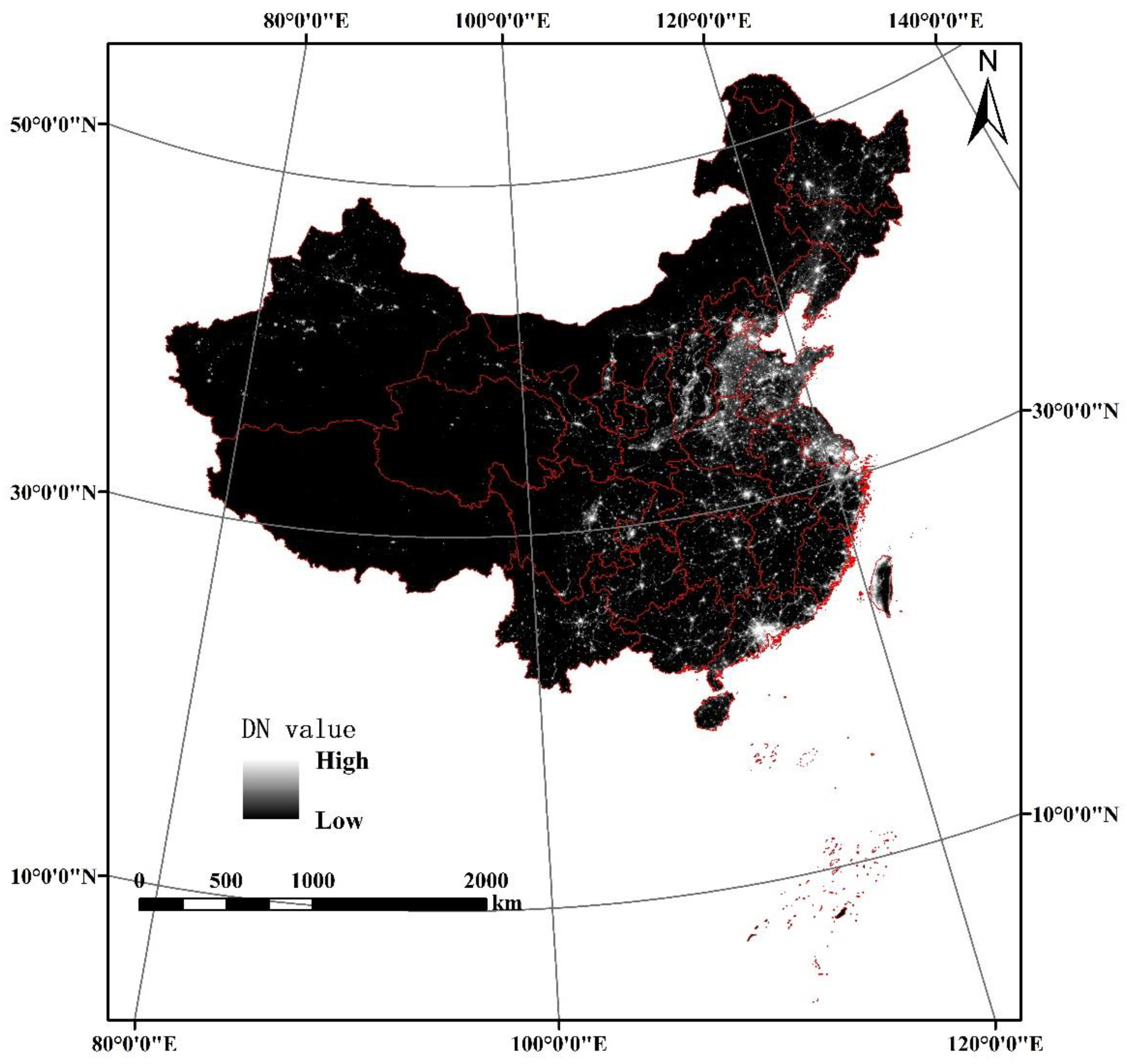
2.1. Study Area
2.2. Data Sources
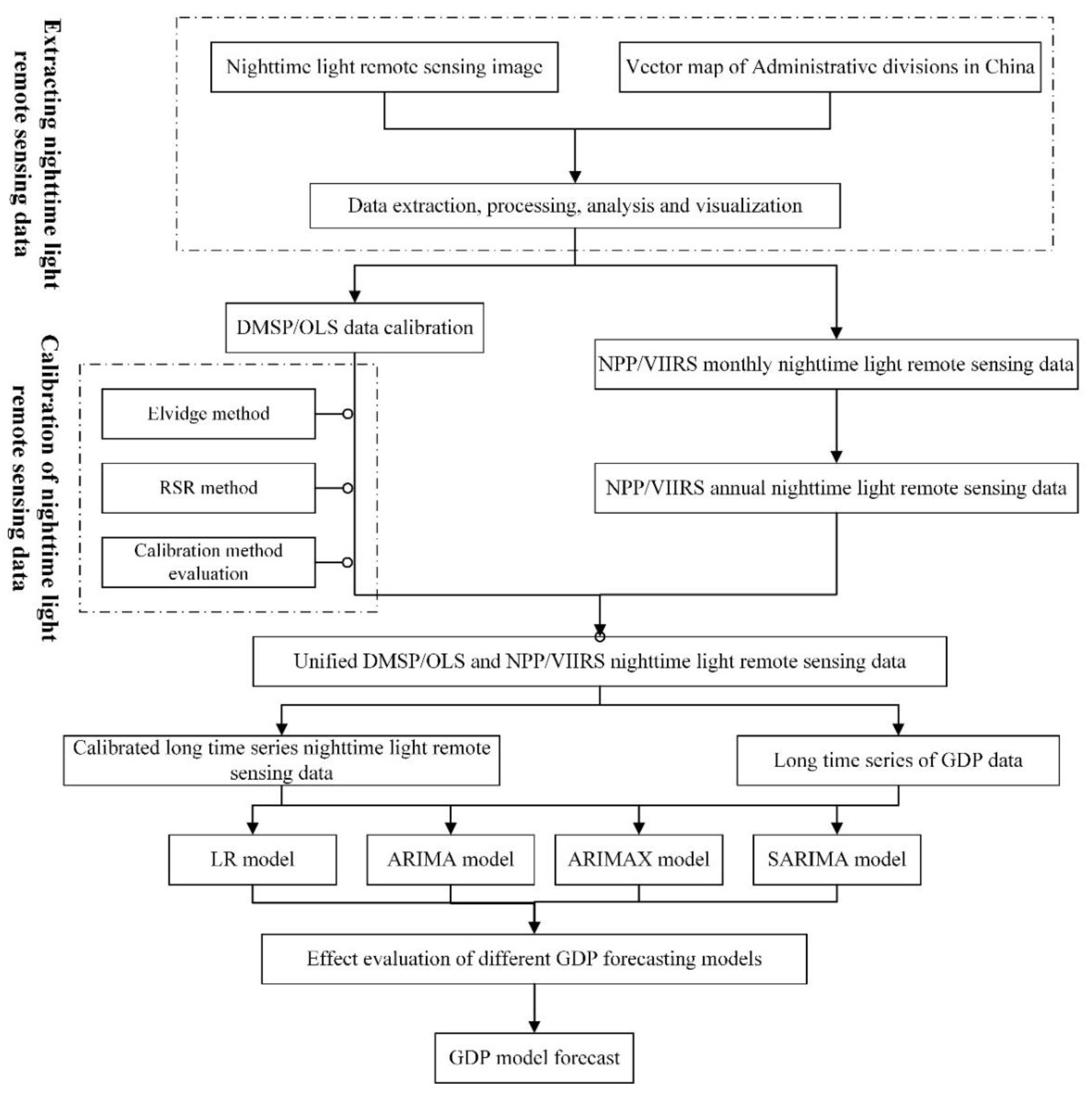
3. Methods
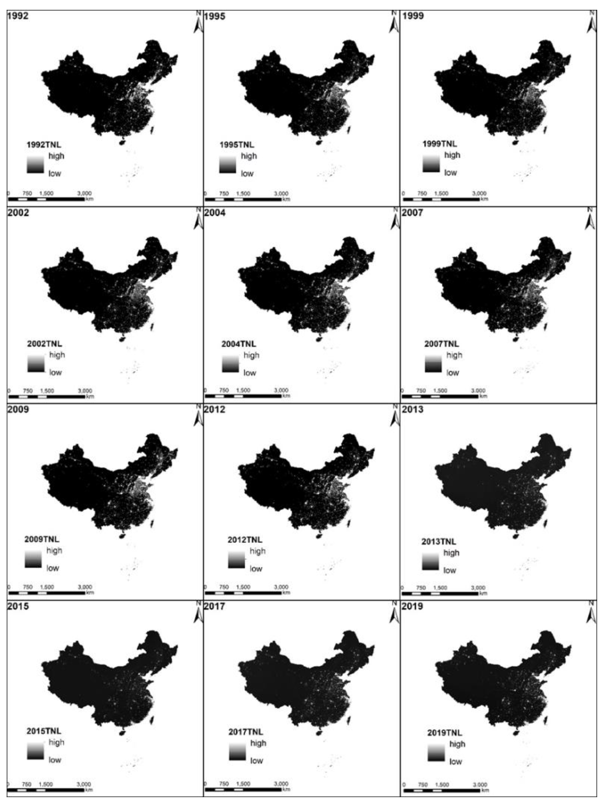
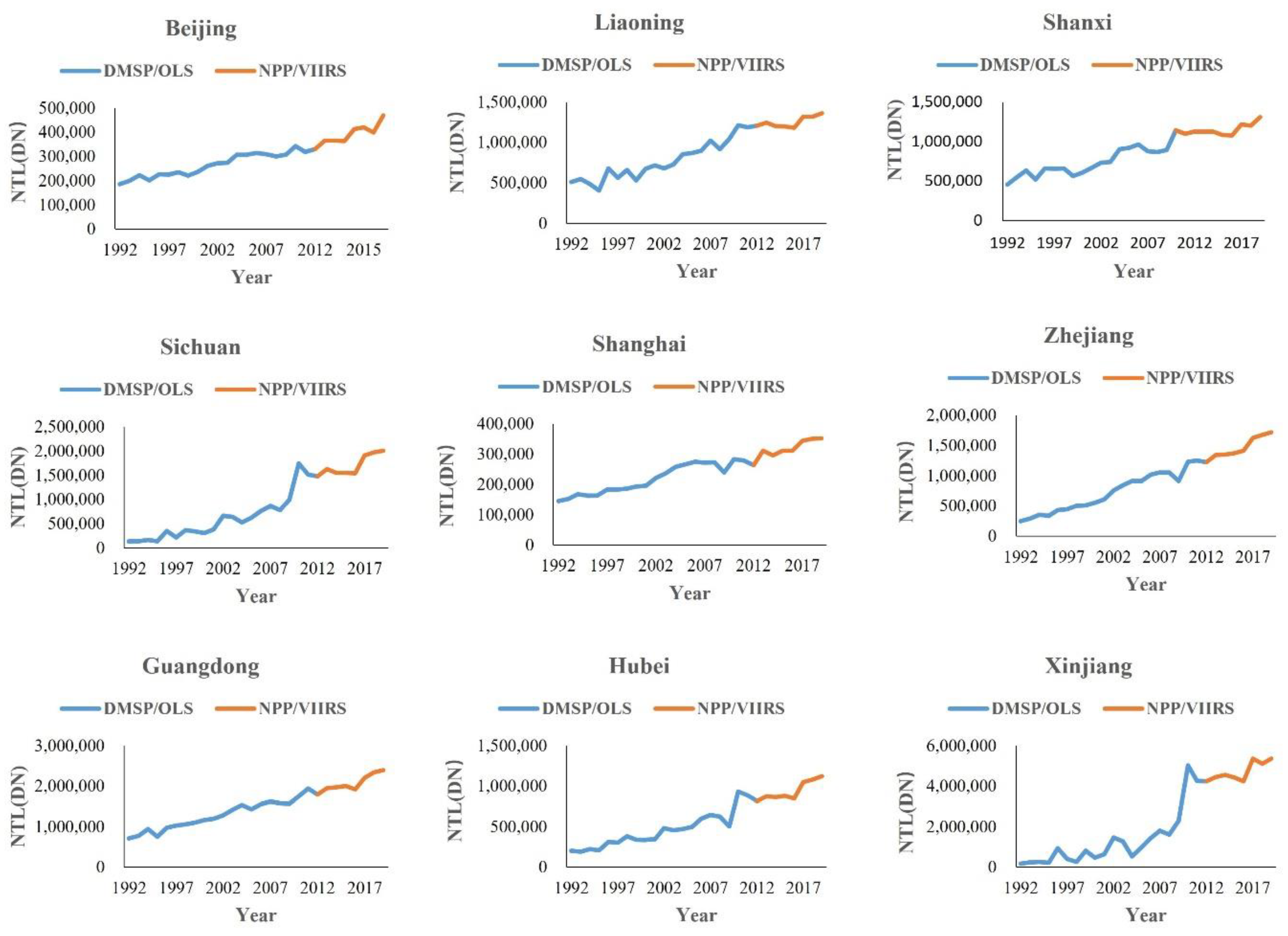
3.1. Establishing Consistent Long NTL Time Series
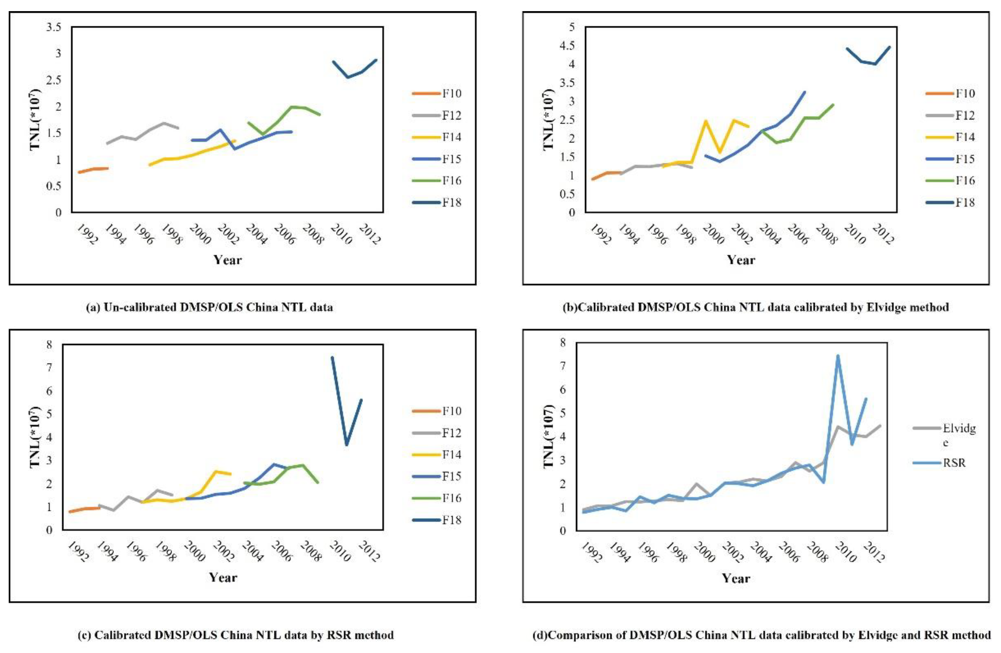
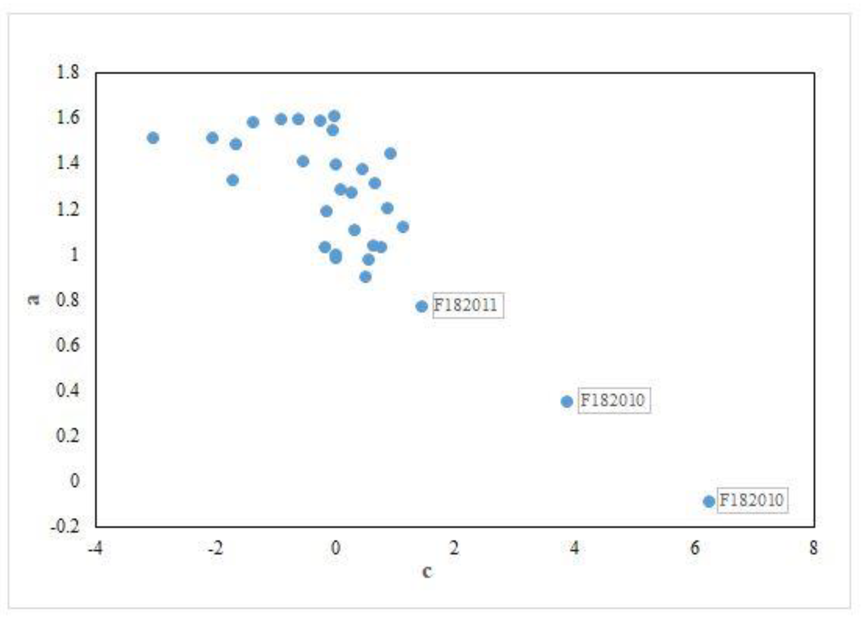
3.1.1. Internal Calibration of DMSP/OLS
3.1.2. Cross-Sensor Calibration of DMSP/OLS and NPP/VIIRS
3.2. GDP Forecasting Model
3.2.1. Linear Regression (LR) Model
3.2.2. ARIMA Model
3.2.3. ARIMAX Model
3.2.4. SARIMA Model
3.3. Accuracy Evaluation
4. Results
4.1. The Calibration of the NTL
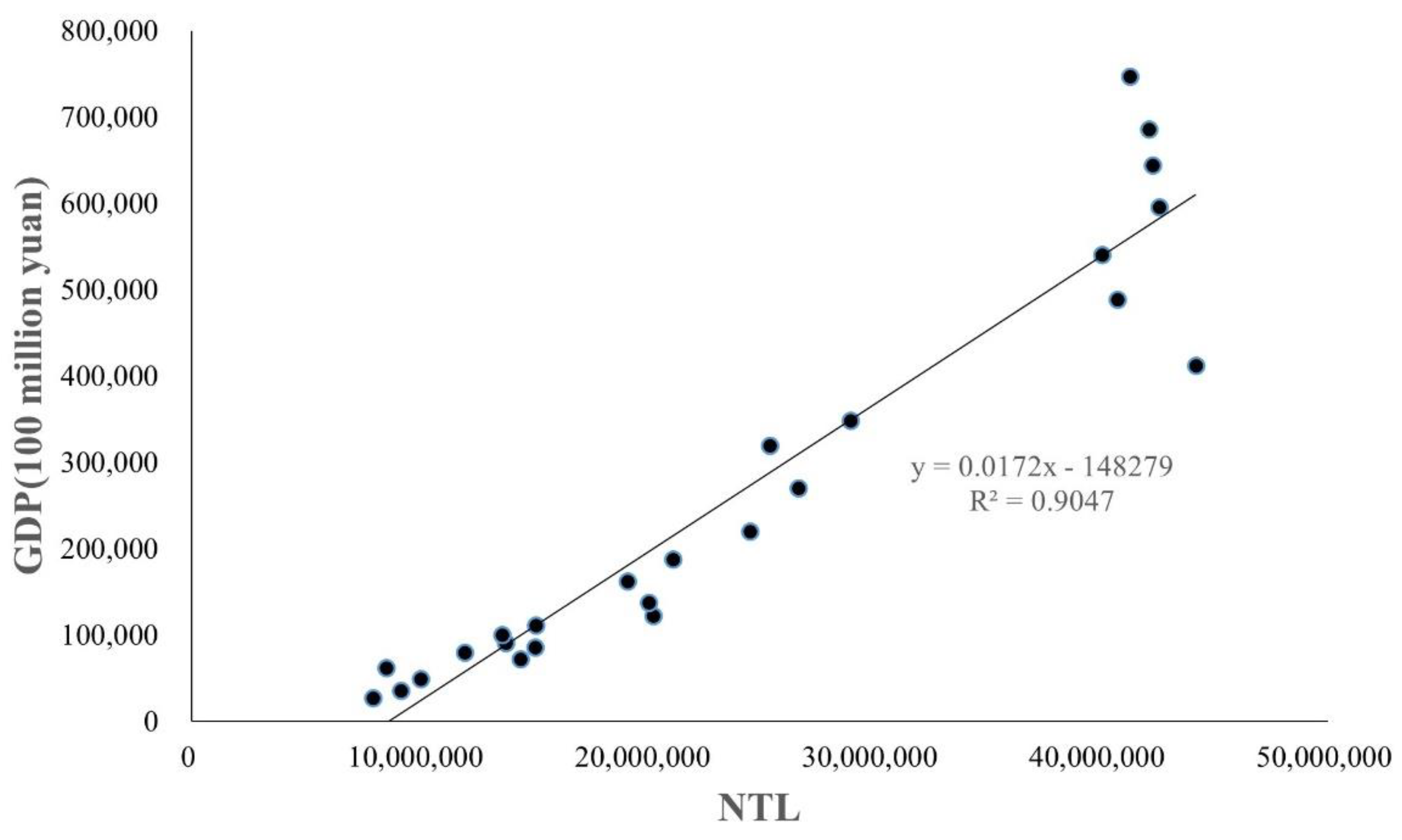
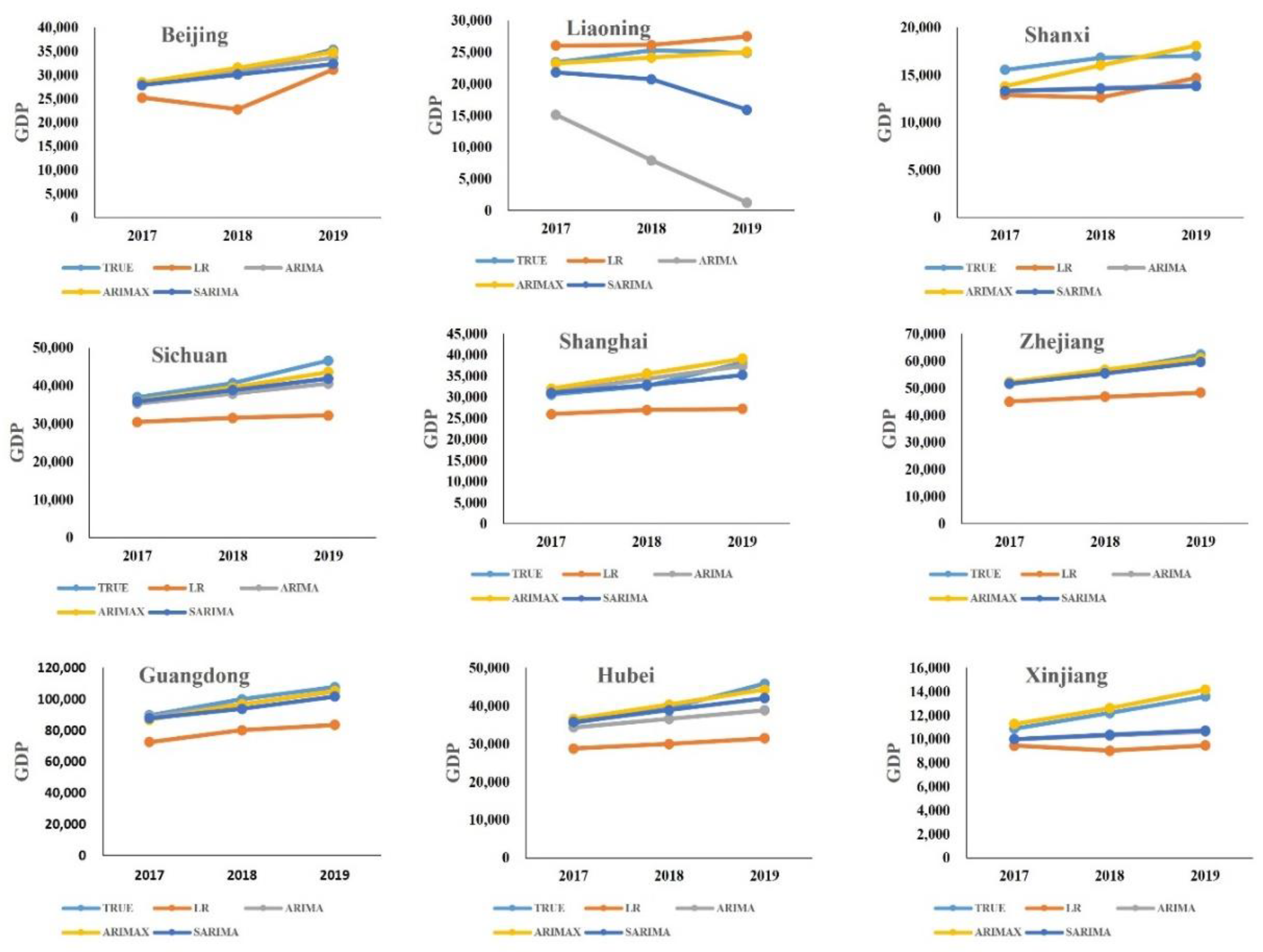
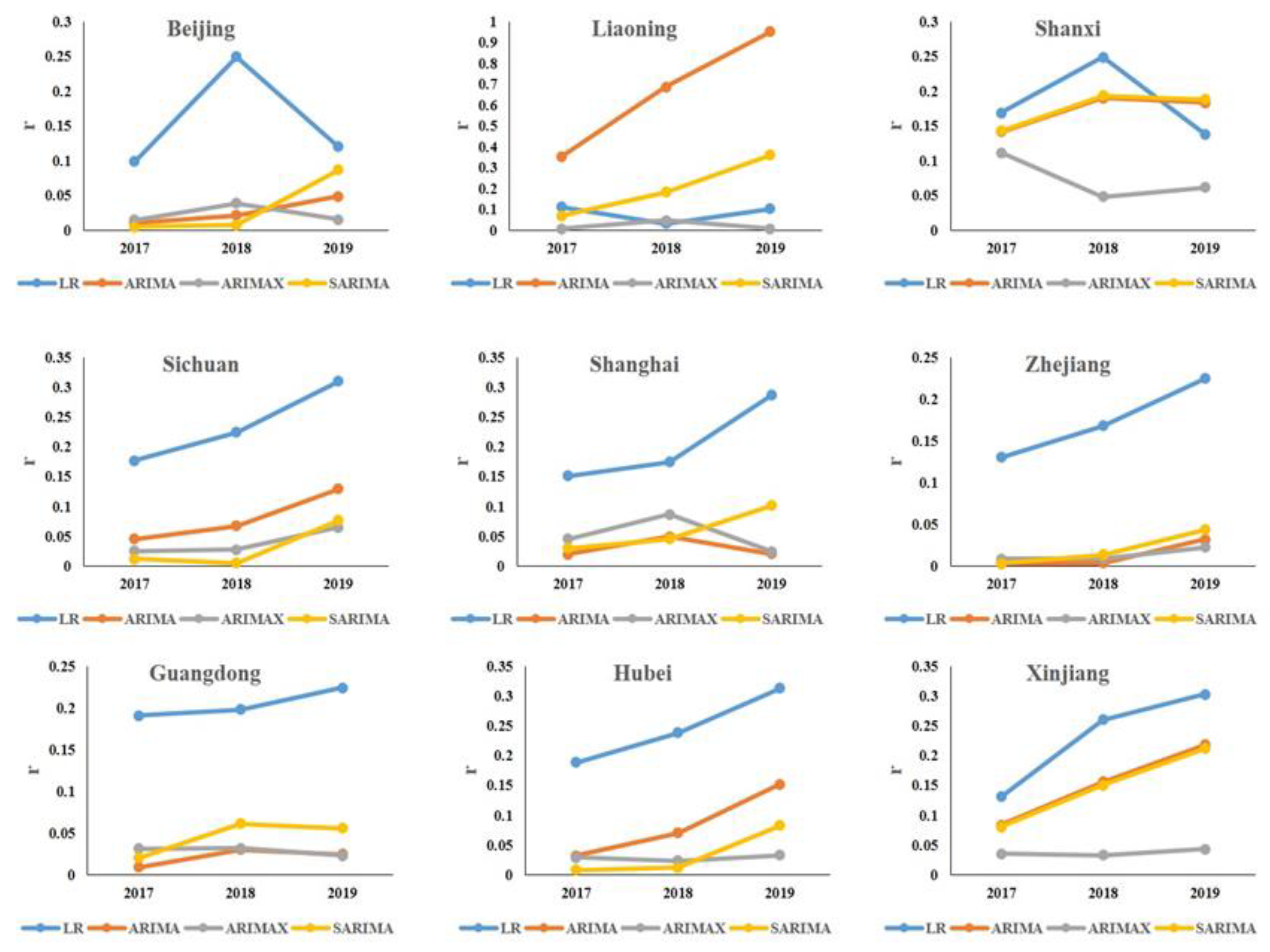
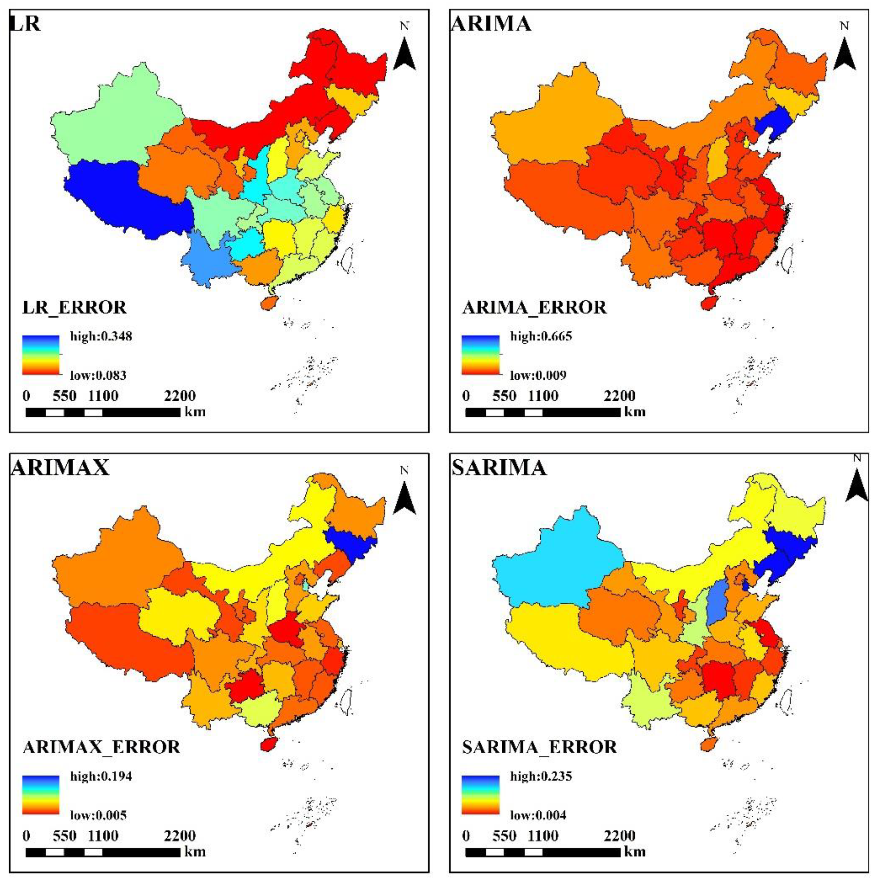
4.2. NTL–GDP Relationship and Model Evaluation
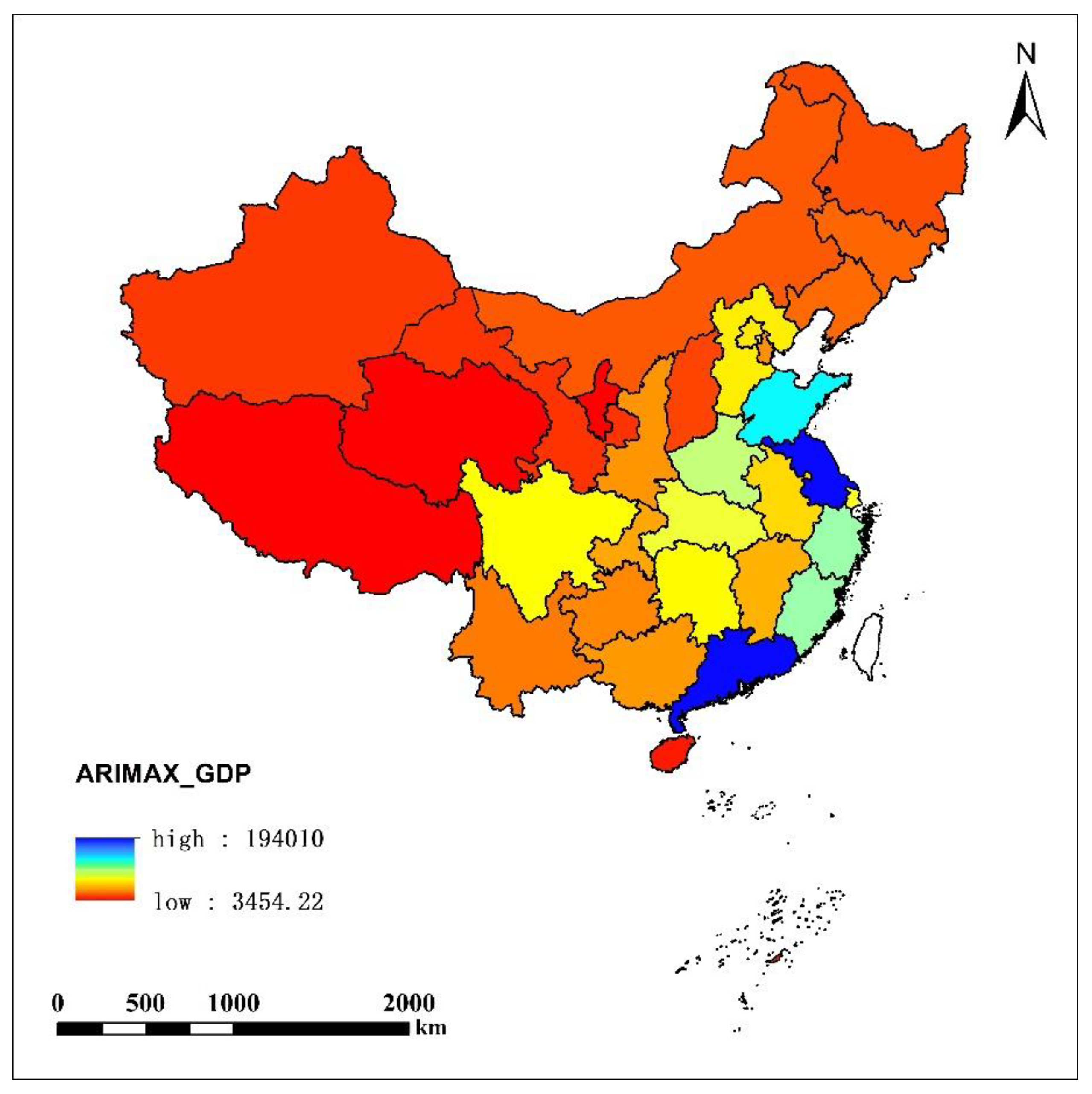
4.3. GDP Forecast in 2030
5. Discussion
5.1. Time Change of GDP
5.2. Spatial Variation of GDP
5.3. Limitation Analysis
6. Conclusions
Author Contributions
Funding
Data Availability Statement
Acknowledgments
Conflicts of Interest
References
- Chen, X.; Nordhaus, W. VIIRS Nighttime Lights in the Estimation of Cross-Sectional and Time-Series GDP. Remote Sens. 2019, 11, 1057. [Google Scholar] [CrossRef] [Green Version]
- Cai, B.; Shao, Z.; Fang, S.; Huang, X. Quantifying Dynamic Coupling Coordination Degree of Human–Environmental Interactions during Urban–Rural Land Transitions of China. Land 2022, 11, 935. [Google Scholar] [CrossRef]
- Li, Z.; Jiao, L.; Zhang, B.; Xu, G.; Liu, J. Understanding the pattern and mechanism of spatial concentration of urban land use, population and economic activities: A case study in Wuhan, China. Geo-Spat. Inf. Sci. 2021, 24, 678–694. [Google Scholar] [CrossRef]
- Zhuang, Q.; Shao, Z.; Li, D.; Huang, X.; Cai, B.; Altan, O.; Wu, S. Unequal weakening of urbanization and soil salinization on vegetation production capacity. Geoderma 2022, 411, 115712. [Google Scholar] [CrossRef]
- Marc, F.; Philippe, M. The news of the death of welfare economics is greatly exaggerated. Soc. Choice Welf. 2005, 25, 381–418. [Google Scholar] [CrossRef] [Green Version]
- Huh, H.; Chung, M. A method to allocate GDP statistical discrepancy. Appl. Econ. Lett. 2006, 13, 587–591. [Google Scholar] [CrossRef]
- Zhang, X.; Guo, S.; Guan, Y.; Cai, D.; Zhang, C.; Fraedrich, K.; Xiao, H.; Tian, Z. Urbanization and Spillover Effect for Three Megaregions in China: Evidence from DMSP/OLS Nighttime Lights. Remote Sens. 2018, 10, 1888. [Google Scholar] [CrossRef] [Green Version]
- Xu, P.; Jin, P.; Yang, Y.; Wang, Q.; Bagan, H. Evaluating Urbanization and Spatial-Temporal Pattern Using the DMSP/OLS Nighttime Light Data: A Case Study in Zhejiang Province. Math. Probl. Eng. 2016, 2016, 9850890. [Google Scholar] [CrossRef] [Green Version]
- Cai, B.; Shao, Z.; Fang, S.; Huang, X.; Huq, M.E.; Tang, Y.; Li, Y.; Zhuang, Q. Finer-scale spatiotemporal coupling coordination model between socioeconomic activity and eco-environment: A case study of Beijing, China. Ecol. Indic. 2021, 131, 108165. [Google Scholar] [CrossRef]
- Li, X.; Liu, S.; Jendryke, M.; Li, D.; Wu, C. Night-Time Light Dynamics during the Iraqi Civil War. Remote Sens. 2018, 10, 858. [Google Scholar] [CrossRef] [Green Version]
- Shao, Z.; Tang, Y.; Huang, X.; Li, D. Monitoring Work Resumption of Wuhan in the COVID-19 Epidemic Using Daily Nighttime Light. Photogramm. Eng. Remote Sens. 2021, 87, 197–206. [Google Scholar] [CrossRef]
- Elvidge, C.; Ziskin, D.; Baugh, K.; Tuttle, B.; Ghosh, T.; Pack, D.; Erwin, E.; Zhizhin, M. A Fifteen Year Record of Global Natural Gas Flaring Derived from Satellite Data. Energies 2009, 2, 595–622. [Google Scholar] [CrossRef]
- Fu, H.; Shao, Z.; Fu, P.; Cheng, Q.; Yu, B.; Thenkabail, P. The Dynamic Analysis between Urban Nighttime Economy and Urbanization Using the DMSP/OLS Nighttime Light Data in China from 1992 to 2012. Remote Sens. 2017, 9, 416. [Google Scholar] [CrossRef] [Green Version]
- Gonzales, F.; London, S.; Santos, M. Disasters and economic growth: Evidence for Argentina. Clim. Dev. 2021, 13, 932–943. [Google Scholar] [CrossRef]
- Li, X.; Cai, G.; Luo, D. GDP distortion and tax avoidance in local SOEs: Evidence from China. Int. Rev. Econ. Financ. 2020, 69, 582–598. [Google Scholar] [CrossRef]
- Galimberti, J. Forecasting GDP Growth from Outer Space. Oxf. Bull. Econ. Stat. 2020, 82, 697–722. [Google Scholar] [CrossRef] [Green Version]
- Sun, J.; Di, L.; Sun, Z.; Wang, J.; Wu, Y. Estimation of GDP Using Deep Learning with NPP-VIIRS Imagery and Land Cover Data at the County Level in CONUS. IEEE J. Sel. Top. Appl. Earth Obs. Remote Sens. 2020, 13, 1400–1415. [Google Scholar] [CrossRef]
- Liang, H.; Guo, Z.; Wu, J.; Chen, Z. GDP spatialization in Ningbo City based on NPP/VIIRS night-time light and auxiliary data using random forest regression. Adv. Space Res. 2020, 65, 481–493. [Google Scholar] [CrossRef]
- Ma, C.; Niu, Y.; Ma, Y.; Chen, F.; Yang, J.; Liu, J. Assessing the Distribution of Heavy Industrial Heat Sources in India between 2012 and 2018. ISPRS Int. J. Geo-Inf. 2020, 8, 568. [Google Scholar] [CrossRef] [Green Version]
- Zhang, E.; Feng, H.; Peng, S.; Gary, A. Measurement of Urban Expansion and Spatial Correlation of Central Yunnan Urban Agglomeration Using Nighttime Light Data. Math. Probl. Eng. 2021, 2021, 8898468. [Google Scholar] [CrossRef]
- Levin, N.; Kyba, C.; Zhang, Q.; Miguel, A.; Román, M.; Li, X.; Portnov, B.; Molthan, A.; Jechow, A.; Miller, S.; et al. Remote sensing of night lights: A review and an outlook for the future. Remote Sens. Environ. 2020, 237, 111443. [Google Scholar] [CrossRef]
- Li, X.; Li, D. Can night-time light images play a role in evaluating the Syrian Crisis? Int. J. Remote Sens. 2014, 35, 6648–6661. [Google Scholar] [CrossRef]
- Gu, Y.; Shao, Z.; Huang, X.; Fu, Y.; Gao, J.; Fan, Y. Assessing the Impact of Land Use Changes on Net Primary Productivity in Wuhan, China. Photogramm. Eng. Remote Sens. 2022, 88, 189–197. [Google Scholar] [CrossRef]
- Bayan, A.; Ryutaro, T.; Dong, X.; Nguyen, T.; Ahmad, A.; Bai, X. New urban map of Eurasia using MODIS and multi-source geospatial data. Geo-Spat. Inf. Sci. 2017, 20, 29–38. [Google Scholar] [CrossRef] [Green Version]
- Weidmann, N.; Theunissen, G. Estimating Local Inequality from Nighttime Lights. Remote Sens. 2021, 13, 4642. [Google Scholar] [CrossRef]
- Peled, Y.; Fishman, T. Estimation and mapping of the material stocks of buildings of Europe: A novel nighttime lights-based approach. Resour. Conserv. Recycl. 2021, 169, 105509. [Google Scholar] [CrossRef]
- Oda, T.; Román, M.; Wang, Z.; Stokes, E.; Sun, Q.; Shrestha, R.; Feng, S.; Lauvaux., T.; Bun, R.; Maksyutov, S.; et al. US Cities in the Dark: Mapping Man-Made Carbon Dioxide Emissions Over the Contiguous US Using NASA’s Black Marble Nighttime Lights Product. In Urban Remote Sensing: Monitoring, Synthesis, and Modeling in the Urban Environment, 2nd ed.; Yang, X., Ed.; Wuhan University: Wuhan, China, 2021; pp. 337–367. [Google Scholar] [CrossRef]
- Straka, T.; Wolf, M.; Gras, P.; Buchholz, S.; Voigt, C. Tree cover mediates the effect of artificial light on urban bats. Front. Ecol. Evol. 2019, 7, 91. [Google Scholar] [CrossRef] [Green Version]
- James, P.; Bertrand, K.; Hart, J.; Schernhammer, E.; Tamimi, R.; Laden, F. Outdoor light at night and breast cancer incidence in the nurses’ health study II. Environ. Health Perspect. 2017, 125, 087010. [Google Scholar] [CrossRef] [Green Version]
- Shao, Z.; Chong, L. The Integrated Use of DMSP-OLS Nighttime Light and MODIS Data for Monitoring Large-Scale Impervious Surface Dynamics: A Case Study in the Yangtze River Delta. Remote Sens. 2014, 6, 9359–9378. [Google Scholar] [CrossRef] [Green Version]
- Ledolter, J.; Box, G. Conditions for the optimality of exponential smoothing forecast procedures. Springer Nat. J. 1978, 25, 77–93. [Google Scholar] [CrossRef] [Green Version]
- Lim, W.; To, W. The economic impact of a global pandemic on the tourism economy: The case of COVID-19 and Macao’s destination- and gambling-dependent economy. Curr. Issues Tour. 2021, 25, 1258–1269. [Google Scholar] [CrossRef]
- Kumar, K.; Paramanik, R. Nexus between Indian Economic Growth and Financial Development: A Non-Linear ARDL Approach. J. Asian Financ. Econ. Bus. 2020, 7, 109–116. [Google Scholar] [CrossRef]
- Shuai, Y.; Zhou, Z. GDP Analysis and Comparison in Coastal Cities Based on Time Series Analysis. J. Coast. Res. 2019, 98, 402–406. [Google Scholar] [CrossRef]
- Zou, J.; Bui, K.; Xiao, Y.; Doan, C. Dam deformation analysis based on BPNN merging models. Geo-Spat. Inf. Sci. 2018, 21, 149–157. [Google Scholar] [CrossRef] [Green Version]
- Miah, M.; Tabassum, M.; Rana, M. Modelling and Forecasting of GDP in Bangladesh: An ARIMA Approach. J. Mech. Contin. Math. Sci. 2019, 14, 150–166. [Google Scholar] [CrossRef]
- Zhu, Y.; Wang, Y.; Liu, T.; Sui, Q. Assessing macroeconomic recovery after a natural hazard based on ARIMA—A case study of the 2008 Wenchuan earthquake in China. Nat. Hazards 2018, 91, 1025–1038. [Google Scholar] [CrossRef]
- Ediger, V.; Akar, S. ARIMA forecasting of primary energy demand by fuel in Turkey. Energy Policy 2007, 35, 1701–1708. [Google Scholar] [CrossRef]
- Ma, L.; Hu, C.; Lin, R.; Han, Y. ARIMA model forecast based on EViews software. In Proceedings of the International Conference on Air Pollution and Environmental Engineering 2018, Hong Kong, China, 26–28 October 2018. [Google Scholar] [CrossRef]
- Zhao, N.; Cao, G.; Zhang, W.; Samson, E.; Chen, Y. Remote sensing and social sensing for socioeconomic systems: A comparison study between nighttime lights and location-based social media at the 500 m spatial resolution. Int. J. Appl. Earth Obs. Geoinf. 2020, 87, 102058. [Google Scholar] [CrossRef]
- Dong, K.; Li, X.; Cao, H.; Tong, Z. Intercalibration Between Night-Time DMSP/OLS Radiance Calibrated Images and NPP/VIIRS Images Using Stable Pixels. IEEE J. Sel. Top. Appl. Earth Obs. Remote Sens. 2021, 14, 8838–8848. [Google Scholar] [CrossRef]
- Elvidge, C.; Hsu, F.; Baugh, K.; Ghosh, T.; Weng, Q. National Trends in Satellite-Observed Lighting: 1992–2012. Remote Sens. Appl. Ser. 2014, 23, 97–118. [Google Scholar] [CrossRef]
- Zhang, Q.; Pandey, B.; Seto, K. A robust method to generate a consistent time series from DMSP/OLS nighttime light data. IEEE Trans. Geosci. Remote Sens. 2016, 54, 5821–5831. [Google Scholar] [CrossRef]
- Zheng, Q.; Weng, Q.; Wang, K. Developing a new cross-sensor calibration model for DMSP-OLS and Suomi-NPP VIIRS night-light imageries. ISPRS J. Photogramm. Remote Sens. 2019, 153, 36–47. [Google Scholar] [CrossRef]
- Green, J.; Perkins, C.; Steinbach, R.; Edwards, P. Reduced street lighting at night and health: A rapid appraisal of public views in England and Wales. Health Place 2015, 34, 171–180. [Google Scholar] [CrossRef] [PubMed] [Green Version]
- Altan, O.; Dowman, I. The changing world under the corona virus threat—from human needs to SDGs and what next? Geo-Spat. Inf. Sci. 2021, 24, 50–57. [Google Scholar] [CrossRef]
- Griffith, D.; Li, B. Spatial-temporal modeling of initial COVID-19 diffusion: The cases of the Chinese Mainland and Conterminous United States. Geo-Spat. Inf. Sci. 2021, 24, 340–362. [Google Scholar] [CrossRef]
- Román, M.; Wang, Z.; Sun, Q.; Kalb, V.; Miler, S.; Molthan, A.; Schultz, L.; Bell, J.; Stokes, E.; Pandey, B.; et al. NASA’s Black Marble nighttime lights product suite. Remote Sens. Environ. 2018, 210, 113–143. [Google Scholar] [CrossRef]
- Kyba, C.; Garz, S.; Kuechly, H.; De Miguel, S.; Zamorano, J.; Fischer, J.; Hölker, F. High-resolution imagery of earth at night: New sources, opportunities and challenges. Remote Sens. 2015, 7, 1–23. [Google Scholar] [CrossRef] [Green Version]
- Sánchez de Miguel, A.; Aubé, M.; Zamorano, J.; Kocifaj, M.; Roby, J.; Tapia, C. Sky Quality Meter measurements in a colour-changing world. Mon. Not. R. Astron. Soc. 2017, 467, 2966–2979. [Google Scholar] [CrossRef]


| Sensor | DMSP/OLS | Suomi NPP/VIIRS |
|---|---|---|
| Archive year | 1992–2013 | April 2012- |
| Spatial resolution/m | 2700 | 740 |
| Time resolution/h | 12 | 12 |
| Country | America | America |
| Data accessibility | Free annual video download, monthly average and daily video to order | Monthly average, daily video free download |
| Year | F10 | F12 | F14 | F15 | F16 | F18 |
|---|---|---|---|---|---|---|
| 1992 | F101992 | |||||
| 1993 | F101993 | |||||
| 1994 | F101994 | F121994 | ||||
| 1995 | F121995 | |||||
| 1996 | F121996 | |||||
| 1997 | F121997 | F141997 | ||||
| 1998 | F121998 | F141998 | ||||
| 1999 | F121999 | F141999 | ||||
| 2000 | F142000 | F152000 | ||||
| 2001 | F142001 | F152001 | ||||
| 2002 | F142002 | F152002 | ||||
| 2003 | F142003 | F152003 | ||||
| 2004 | F152004 | F162004 | ||||
| 2005 | F152005 | F162005 | ||||
| 2006 | F152006 | F162006 | ||||
| 2007 | F152007 | F162007 | ||||
| 2008 | F162008 | |||||
| 2009 | F162009 | |||||
| 2010 | F182010 | |||||
| 2011 | F182011 | |||||
| 2012 | F182012 | |||||
| 2013 | F182013 |
| Year | Satellite 1 | Satellite 2 | Raw | Elvidge | RSR | ||
|---|---|---|---|---|---|---|---|
| 1994 | F10 | F12 | 0.023 | 0.015 | 0.052 | ||
| 1997 | F12 | F14 | 0.532 | 0.017 | 0.008 | ||
| 1998 | F12 | F14 | 0.089 | 0.012 | 0.129 | ||
| 1999 | F12 | F14 | 0.077 | 0.054 | 0.099 | ||
| 2000 | F14 | F15 | 0.238 | 0.234 | 0.002 | ||
| 2001 | F14 | F15 | 0.361 | 0.084 | 0.088 | ||
| 2002 | F14 | F15 | 0.241 | 0.221 | 0.242 | ||
| 2003 | F14 | F15 | 0.086 | 0.118 | 0.206 | ||
| 2004 | F15 | F16 | 0.006 | 0.003 | 0.059 | ||
| 2005 | F15 | F16 | 0.079 | 0.108 | 0.064 | ||
| 2006 | F15 | F16 | 0.149 | 0.145 | 0.151 | ||
| 2007 | F15 | F16 | 0.150 | 0.119 | 0.008 | ||
| 2.033 | 1.132 | 1.108 | |||||
| Year | Trillion Yuan | Year | Trillion Yuan | Year | Trillion Yuan | |||
|---|---|---|---|---|---|---|---|---|
| Province | Province | Province | ||||||
| Beijing | 62,832.69 | Tianjin | 36,746.19 | Hebei | 63,771.21 | |||
| Shanxi | 19,321.30 | Neimenggu | 22,280.36 | Liaoning | 26,416.12 | |||
| Jilin | 24,768.18 | Heilongjiang | 19,619.97 | Shanghai | 71,024.35 | |||
| Jiangsu | 194,010.35 | Zhejiang | 108,359.54 | Anhui | 58,035.48 | |||
| Fujian | 68,441.22 | Jiangxi | 46,614.7 | Shandong | 13,3058.04 | |||
| Henan | 95,018.14 | Hubei | 76,278.04 | Hunan | 68,639.61 | |||
| Guangdong | 193,447.95 | Guangxi | 39,520.92 | Hainan | 8959.36 | |||
| Chongqing | 43,340.22 | Sichuan | 69,464.10 | Guizhou | 35,046.67 | |||
| Yunnan | 31,157.92 | Xizang | 3454.22 | Shaanxi | 38,687.81 | |||
| Gansu | 12,941.07 | Qinghai | 4720.20 | Ningxia | 6764.07 | |||
| Xinjiang | 14,198.30 | |||||||
Publisher’s Note: MDPI stays neutral with regard to jurisdictional claims in published maps and institutional affiliations. |
© 2022 by the authors. Licensee MDPI, Basel, Switzerland. This article is an open access article distributed under the terms and conditions of the Creative Commons Attribution (CC BY) license (https://creativecommons.org/licenses/by/4.0/).
Share and Cite
Gu, Y.; Shao, Z.; Huang, X.; Cai, B. GDP Forecasting Model for China’s Provinces Using Nighttime Light Remote Sensing Data. Remote Sens. 2022, 14, 3671. https://doi.org/10.3390/rs14153671
Gu Y, Shao Z, Huang X, Cai B. GDP Forecasting Model for China’s Provinces Using Nighttime Light Remote Sensing Data. Remote Sensing. 2022; 14(15):3671. https://doi.org/10.3390/rs14153671
Chicago/Turabian StyleGu, Yan, Zhenfeng Shao, Xiao Huang, and Bowen Cai. 2022. "GDP Forecasting Model for China’s Provinces Using Nighttime Light Remote Sensing Data" Remote Sensing 14, no. 15: 3671. https://doi.org/10.3390/rs14153671