

Remote Monitoring of Atmospheric and Hydrophysical Characteristics of the Water Surface Based on Microwave Radiometric Measurements


Abstract
:
1. Introduction
2. Materials and Methods
2.1. Estimates of Atmospheric Characteristics Based on Microwave Radiometry Data
2.2. Estimates of the Main Hydrophysical Characteristics of the Water Surface Based on the Data of Microwave Radiometric Measurements
3. Results and Discussion
3.1. Processing Results of Satellite Measurements for Certain Areas of the Pacific Ocean
- -
- Development and improvement of means for remote sensing of ocean surface and ice fields;
- -
- Development of methods and means of sub-satellite support for space oceanographic systems;
- -
- Accumulation of experience by consumers of satellite information on the use of remote sensing data.
- Tbmax—maximum value of radio brightness temperature;
- k—a parameter that determines the number of thresholds (for example, k = 1.9);
- d is a parameter determined in the following way d = kmax + 1.
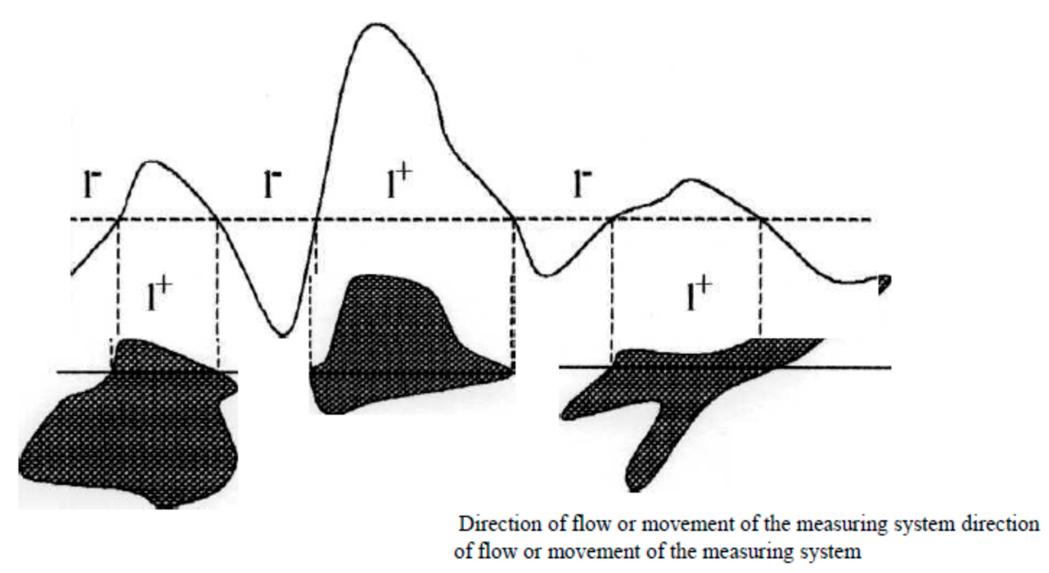
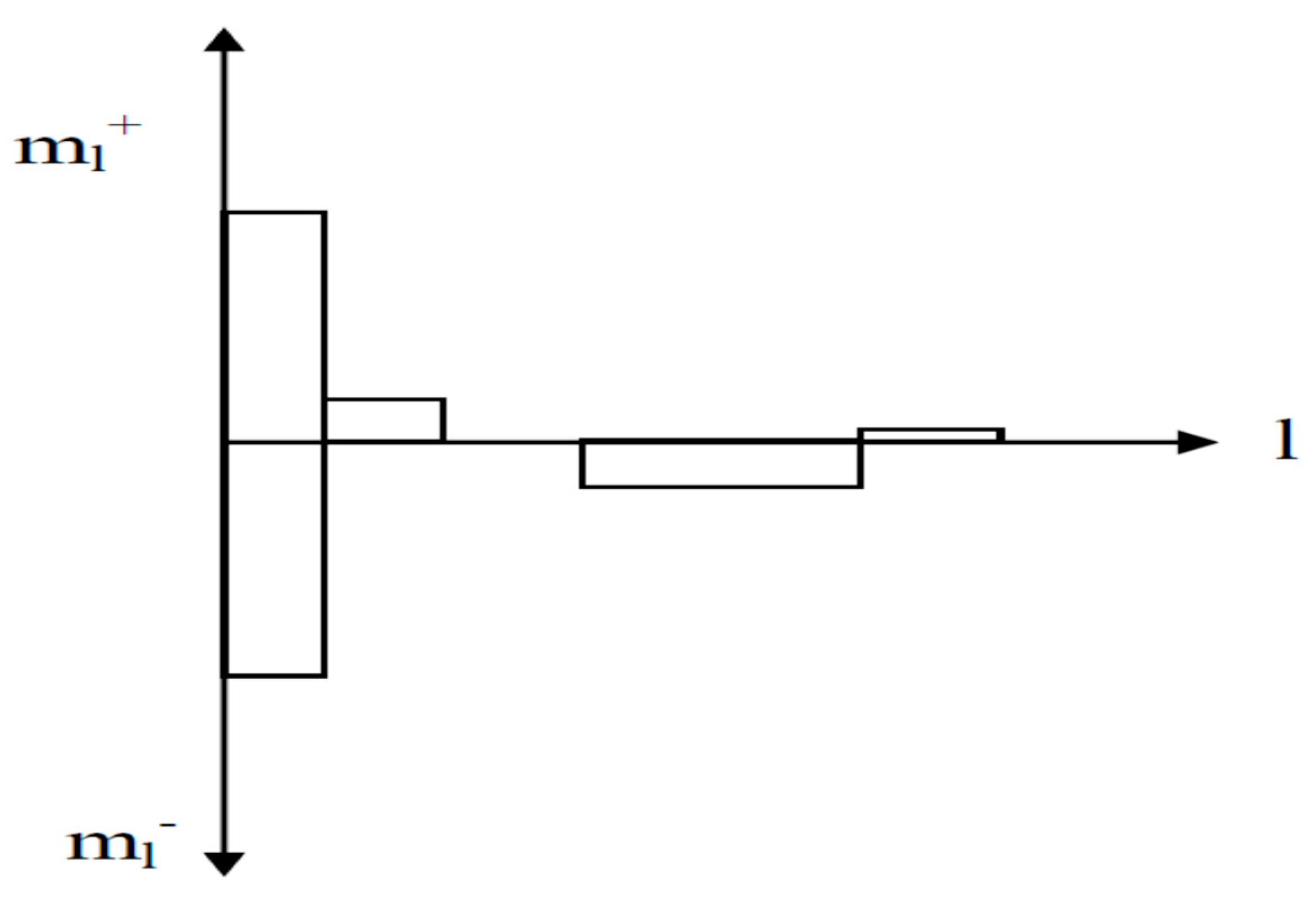
- Tables of statistical characteristics of positive and negative spots (l+, l−)-characteristics).
- Tables of statistical characteristics for average amplitude values of positive and negative “spots”.
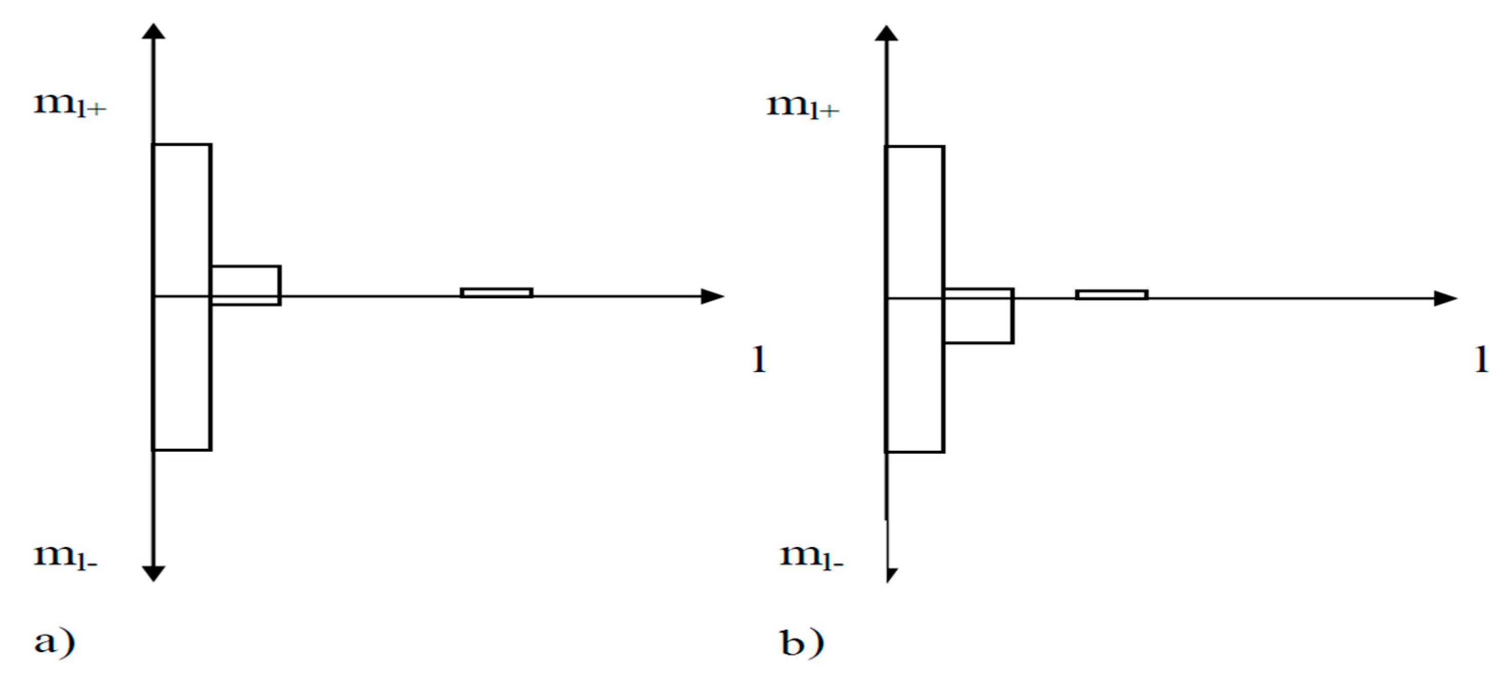
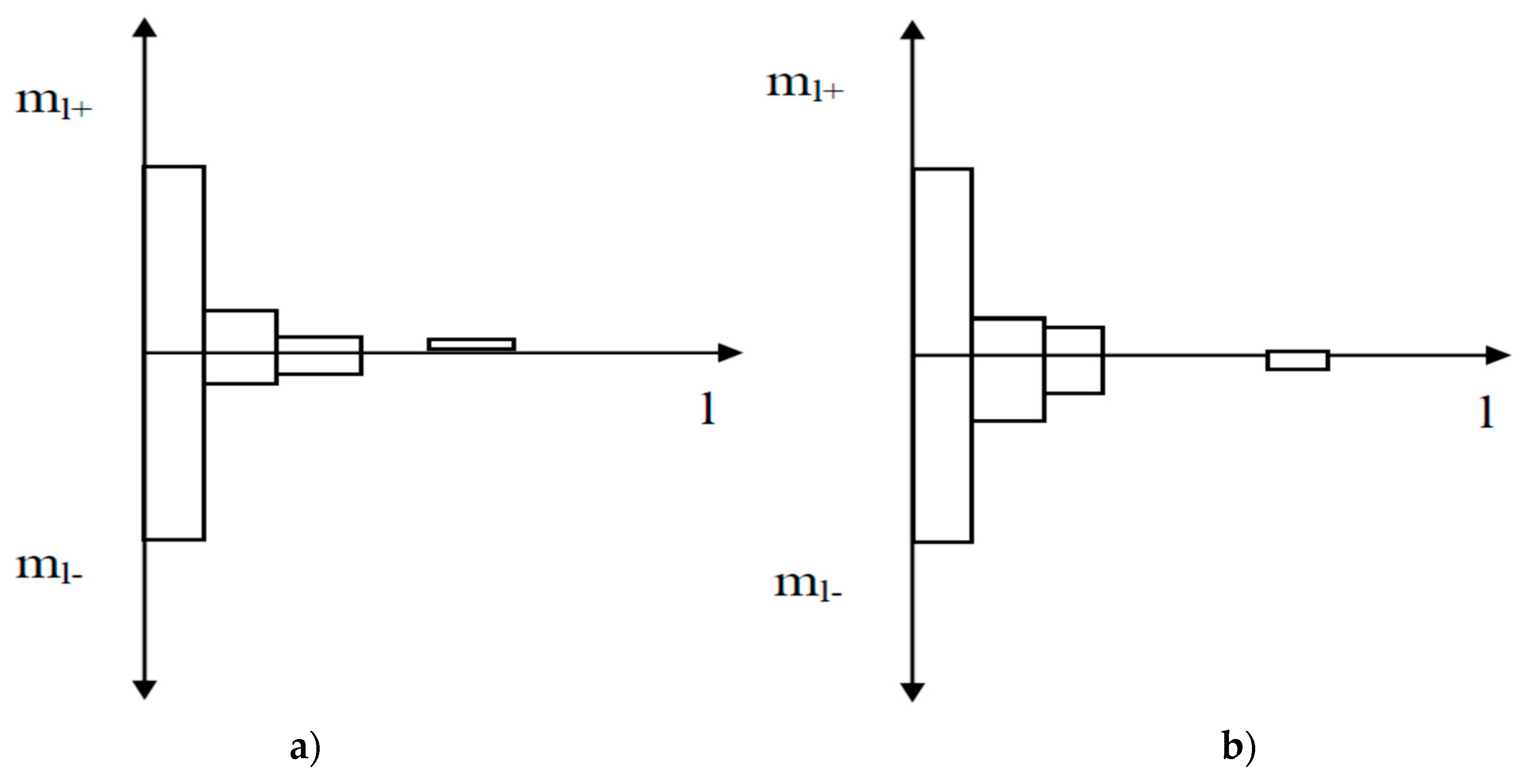
- One-dimensional histograms of (l+, l−)-characteristics (both in terms of the width of the outliers and in terms of the average amplitude values of the outliers).
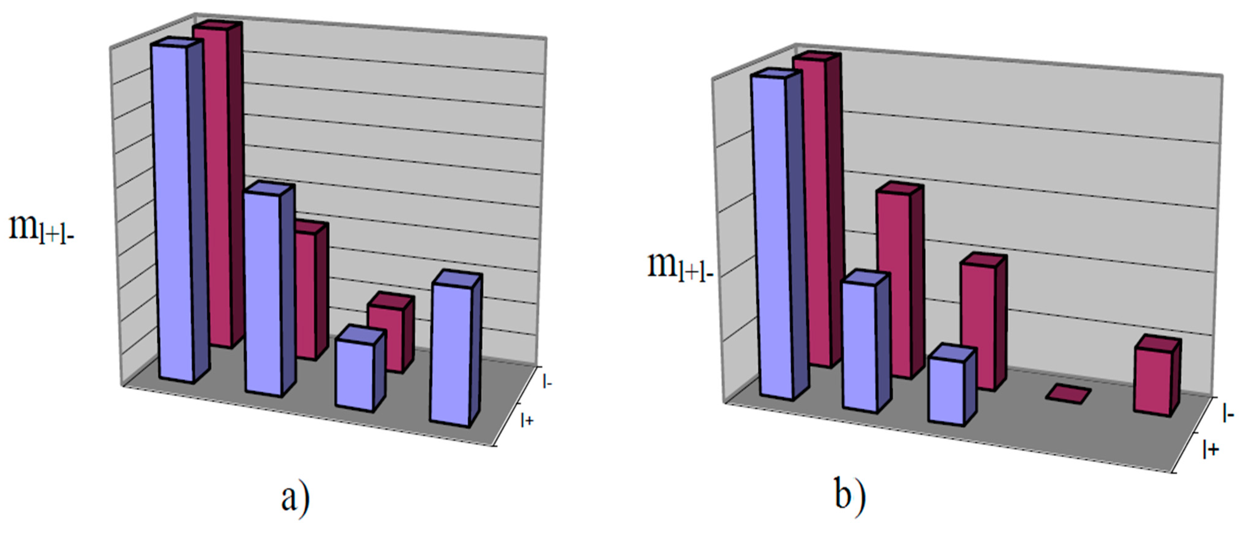
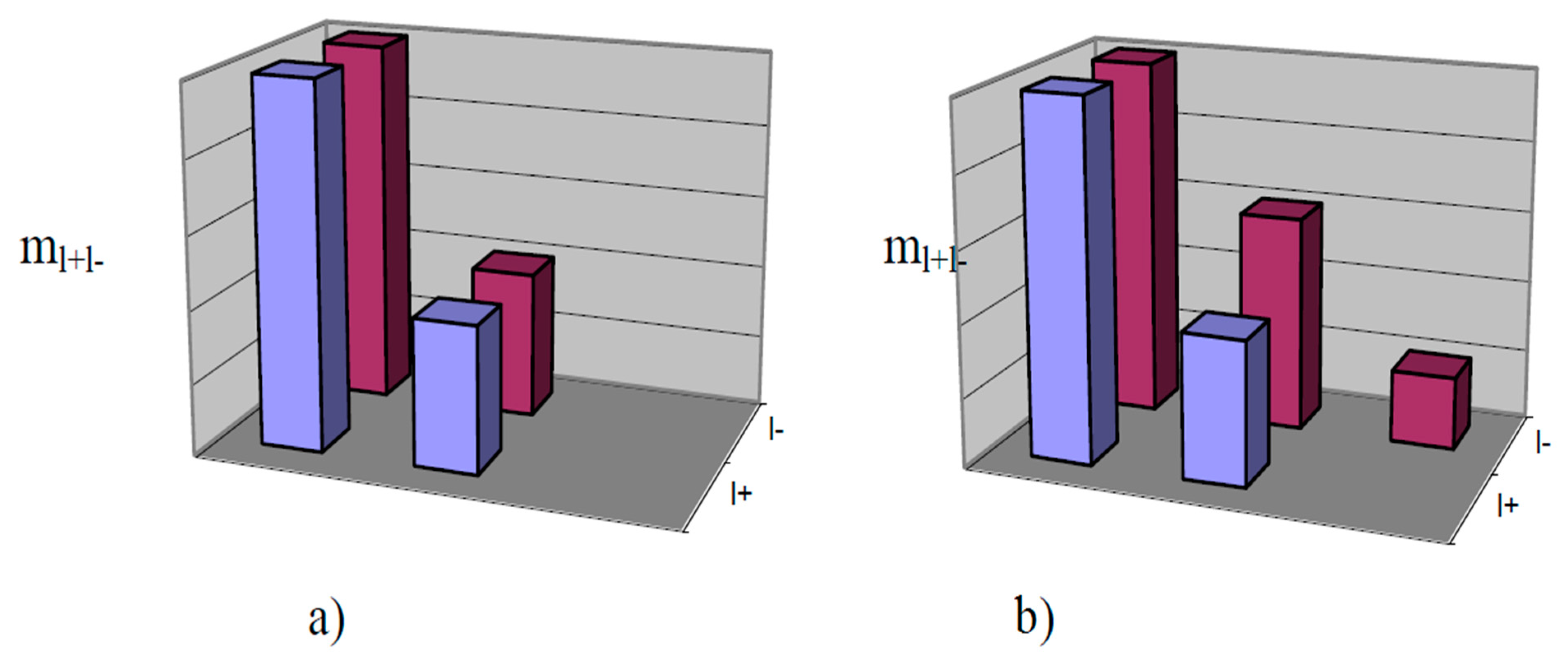
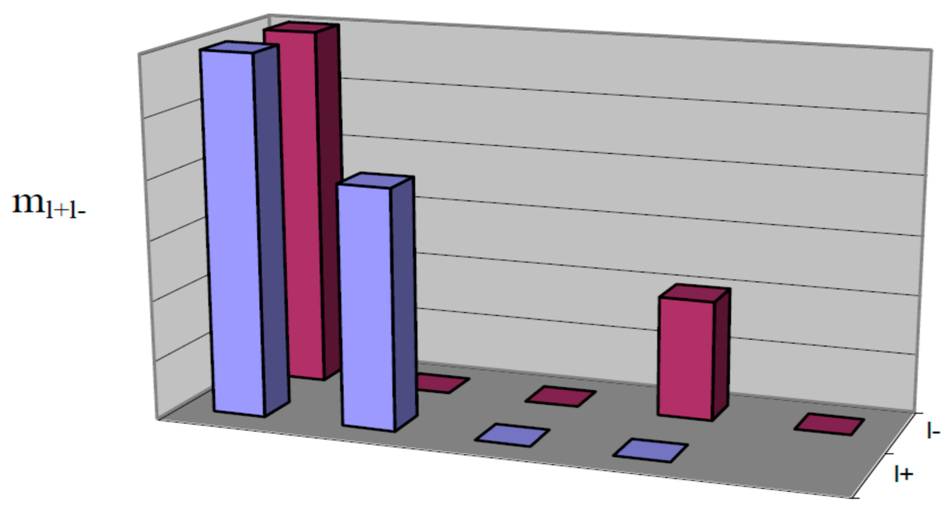
- Two-dimensional histograms (l+, l−)-characteristics (both in terms of the width of the outliers and in terms of the average amplitude values of the outliers).
- Results of the analysis of the joint distribution of (l+, l−)-characteristics for independence.
- Results of the analysis of the distribution type (l+, l−)-characteristics.
3.2. The Case of Calm Surface Water
3.3. The Case of Moderate Surface Water Waves
3.4. The Case of Storm Surface Water Waves
3.5. The Case of Averaged Values
4. Conclusions
Author Contributions
Funding
Acknowledgments
Conflicts of Interest
References
- Armand, N.A.; Savorsky, V.P.; Smirnov, M.T. Study of the earth’s natural resources and environment on the russian segment of the international space station. Mapp. Sci. Remote Sens. 2001, 38, 191–198. [Google Scholar] [CrossRef]
- Afanasiev, Y.A.; Nelepo, B.A.; Selivanov, A.S. Program of experiments “Cosmos-500”. Sov. J. Space 1985, 3–8. [Google Scholar]
- Egorov, D.P.; Kutuza, B.G. Atmospheric brightness temperature fluctuations in the resonance absorption band of water vapor 18–27.2 GHz. IEEE Trans. Geosci. Remote Sens. 2020, 59, 7627–7634. [Google Scholar] [CrossRef]
- Gurvich, A.S.; Egorov, S.T.; Kutuza, B.G. Radiophysical methods of sounding the atmosphere and the surface of the ocean from space. Sov. J. Space 1981, 63–70. [Google Scholar]
- Kutuza, B.G.; Mitnik, L.M.; Akvilonova, A.B. The world’s first experiment on microwave Earth sensing from space on the Kosmos-243 satellite. Curr. Probl. Remote Sens. Earth Space 2019, 16, 9–30. [Google Scholar] [CrossRef]
- Schutko, A.M.; Liberman, B.M.; Chukhray, G. On the influence of dielectric property variations on the microwave radiation of a water surface. IEEE J. Ocean. Ing. 1982, 7, 35. [Google Scholar] [CrossRef]
- Mkrtchyan, F.A. Problems of statistical decisions for remote environmental monitoring. In Proceedings of the SPIE 11501, Earth Observing Systems XXV, 115010R, Online, 24 August–4 September 2020. [Google Scholar]
- Schutko, A.M.; Grankov, A.G. Some peculiarities of formulation and solution of invers problems in the microwave radiometry of the ocean surface and atmosphere. IEEE J. Ocean. Ing. 1982, 7, 40. [Google Scholar] [CrossRef]
- Kutuza, B.G.; Smirnov, M.T. Influence of cloudiness on the average radiothermal radiation of the “atmosphere—ocean surface” system. Sov. J. Space 1980, 76–83. [Google Scholar]
- Malkevich, M.S.; Kosolapov, V.S. On the possibility of remote determination of the vertical moisture profile of clouds. Sov. J. Space 1981, 63–72. [Google Scholar]
- Zhevakin, S.A.; Naumov, A.P. On the calculation of the absorption coefficient of centimeter and millimeter radio waves in atmospheric oxygen. J. Commun. Technol. Electron. 1965, 10, 987–996. [Google Scholar]
- Kalmykov, A.I.; Pichugin, A.P.; Tsymbal, V.N. Determination of the near-water wind field by the side-scan radar system of the Kosmos-1500 satellite. Sov. J. Space 1985, 65–67. [Google Scholar]
- Varotsos, C.A.; Cracknell, A.P. Remote Sensing Letters contribution to the success of the Sustainable Development Goals-UN 2030 agenda. Remote Sens. Lett. 2020, 11, 715–719. [Google Scholar] [CrossRef]
- Nelepo, B.A.; Armand, N.A.; Khmyrov, B.E. The oceanographic experiment involving Cosmos-1076 and Cosmos-1151. Sov. J. Remote Sens. 1984, 2, 383. [Google Scholar]
- Gagarin, S.P.; Kutuza, B.G. Influence of sea roughness and atmospheric inhomogeneities on microwave radiation of the atmosphere–ocean system. IEEE J. Ocean. Eng. 1983, 8, 62–70. [Google Scholar] [CrossRef]
- Grankov, A.G.; Lieberman, B.M.; Shutko, A.M. On the assessment of the physico-chemical parameters of surface waters of water areas by their own microwave radiation. J. Commun. Technol. Electron. 1981, 26, 624. [Google Scholar]
- Krapivin, V.F.; Shutko, A.M. Information Technologies for Remote Monitoring of the Environment; Springer/Praxis: Chichester, UK, 2012; p. 498. [Google Scholar]
- Mkrtchyan, F.A. Problems of Statistical Decisions for Remote Monitoring of the Environment. PIERS 2015 in Prague. In Proceedings of the Progress in Electromagnetics Research Symposium, Prague, Czech Republic, 6–9 July 2015; pp. 639–643. [Google Scholar]
- Mkrtchyan, F.A.; Varotsos, C.A. A New Monitoring System for the Surface Marine Anomalies. Water Air Soil Pollut. 2018, 229, 273. [Google Scholar] [CrossRef]
- Mkrtchyan, F.A.; Shapovalov, S.M. Some aspects of remote monitoring systems of marine ecosystems. Russ. J. Earth Sci. 2018, 18, Es40011-10. [Google Scholar] [CrossRef] [Green Version]
- Kondratyev, K.Y.; Krapivin, V.F.; Savinykh, V.P.; Varotsos, C.A. Global Ecodynamics: A Multidimensional Analysis; Springer-Praxis: Chichester, UK, 2004; 658p. [Google Scholar]
- Krapivin, V.F.; Varotsos, C.A. Biogeochemical Cycles in Globalization and Sustainable Development; Springer/Praxis: Chichester, UK, 2008; 565p. [Google Scholar]
- Krapivin, V.F.; Varotsos, C.A. Globalization and Sustainable Development: Environmental Agendas; Springer/Praxis: Chichester, UK, 2007; 304p. [Google Scholar]
- Basharinov, A.E.; Kutuza, B.G. Investigation of radiation and absorption of cloudy atmosphere in the microwave range. Bull. Am. Meteorol. Soc. 1968, 40, 597. [Google Scholar]
- Mkrtchyan, F.A.; Krapivin, V.F. GIMS-Technology in Monitoring Marine Ecosystems. In Proceedings of the International Symposium of the Photogrammetry, Remote Sensing and Spatial Information Science-Vol XXXVIII, Part 8, Kyoto, Japan, 9–12 August 2010; pp. 427–430. [Google Scholar]
- Cracknell, A.P.; Varotsos, C.A. New aspects of global climate-dynamics research and remote sensing. Int. J. Remote Sens. 2011, 32, 579–600. [Google Scholar] [CrossRef]
- Bettenhausen, M.H.; Smith, G.K.; Bevilacqua, R.M.; Wang, N.Y.; Gaiser, P.W.; Cox, S. Nonlinear Optimization Algorithm for WindSat Wind Vector Retrievals. IEEE Trans. Geosci. Remote Sens. 2006, 44, 597–610. [Google Scholar] [CrossRef]
- Varotsos, C.A.; Krapivin, V.F. Microwave Remote Sensing Tools in Environmental Science; Springer International Publishing: New York, NY, USA, 2020; 468p. [Google Scholar]
- Krapivin, V.F.; Varotsos, C.A. Modelling the CO2 atmosphere-ocean flux in the upwelling zones using radiative transfer tools. J. Atmos. Sol. Terr. Phys. 2016, 150, 47–54. [Google Scholar] [CrossRef]
- Krapivin, V.F.; Mkrtchan, F.A.; Varotsos, C.A.; Xue, Y. Operational diagnosis of arctic waters with instrumental technology and information modeling. Water Air Soil Pollut. 2021, 232, 137. [Google Scholar] [CrossRef]
- Varotsos, C.A. The global signature of the ENSO and SST-like fields. Theor. Appl. Climatol. 2013, 113, 197–204. [Google Scholar] [CrossRef]
- Varotsos, C.A.; Krapivin, V.F. Pollution of Arctic waters has reached a critical point: An innovative approach to this problem. Water Air Soil Pollut. 2018, 229, 343. [Google Scholar] [CrossRef]


| Threshold | Sample Size | M | σ2 | MIN | MAX | RAZ | A | K | ρ | |
|---|---|---|---|---|---|---|---|---|---|---|
| 147.8 | 13 | + | 11 | 326 | 1 | 69 | 68 | 2.53 | 5.27 | −0.101 |
| − | 1.08 | 0.08 | 1 | 2 | 1 | 3.02 | 7.09 | |||
| 149.6 | 18 | + | 6.72 | 162.31 | 1 | 54 | 53 | 2.99 | 7.84 | 0.074 |
| − | 2.06 | 3.7 | 1 | 9 | 8 | 2.74 | 7.07 | |||
| 151.4 | 19 | + | 4.79 | 116.9 | 1 | 48 | 47 | 3.4 | 10.52 | −0.234 |
| − | 3.61 | 7.9 | 1 | 13 | 12 | 1.87 | 4.17 | |||
| 153.2 | 9 | + | 6.56 | 205.36 | 1 | 47 | 46 | 2.45 | 4.07 | −0.266 |
| − | 12.13 | 107.61 | 3 | 34 | 31 | 1.16 | −0.16 | |||
| Threshold | Sample Size | M | σ2 | MIN | MAX | RAZ | A | K | ρ | |
|---|---|---|---|---|---|---|---|---|---|---|
| 159.9 | 16 | + | 12.31 | 257.09 | 1 | 61 | 60 | 1.82 | 2.66 | −0.351 |
| − | 1.4 | 0.37 | 1 | 3 | 2 | 1.26 | 0.51 | |||
| 161.8 | 35 | + | 4.09 | 23.79 | 1 | 22 | 21 | 2.45 | 5.66 | −0.198 |
| − | 2.21 | 5.28 | 1 | 13 | 12 | 3.31 | 11.99 | |||
| 163.7 | 37 | + | 1.81 | 3.5 | 1 | 11 | 10 | 3.46 | 13.23 | −0.020 |
| − | 4.08 | 35.16 | 1 | 34 | 33 | 3.67 | 14.95 | |||
| 165.6 | 8 | + | 2.57 | 3.10 | 1 | 6 | 5 | 0.82 | −0.61 | −0.266 |
| − | 25 | 1268.5 | 1 | 117 | 116 | 2.06 | 2.63 | |||
| Threshold | Sample Size | M | σ2 | MIN | MAX | RAZ | A | K | ρ | |
|---|---|---|---|---|---|---|---|---|---|---|
| 162 | 6 | + | 13.5 | 333.25 | 1 | 52 | 51 | 1.42 | 0.39 | 0.1 |
| − | 1.5 | 1.25 | 1 | 4 | 3 | 1.79 | 1.2 | |||
| 163.5 | 12 | + | 5.5 | 157.25 | 1 | 47 | 46 | 2.99 | 7.01 | 0.034 |
| − | 2 | 1 | 1 | 4 | 3 | 0.5 | −1 | |||
| 166.5 | 7 | + | 7.5 | 96.58 | 1 | 29 | 28 | 1.63 | 0.89 | 0.16 |
| − | 7.5 | 86.58 | 1 | 23 | 22 | 0.78 | −1.29 | |||
| Threshold | Sample Size | M | σ2 | MIN | MAX | RAZ | A | K | ρ | |
|---|---|---|---|---|---|---|---|---|---|---|
| 147.8 | 13 | + | 150.55 | 3.71 | 148.7 | 155.9 | 7.2 | 1.5 | 1.97 | −0.373 |
| − | 146.7 | 0.87 | 144.2 | 147.2 | 3 | −1.68 | 1.53 | |||
| 149.6 | 18 | + | 151.3 | 2.86 | 150.2 | 157.5 | 7.3 | 2.67 | 6.98 | 0.21 |
| − | 148 | 0.93 | 145.7 | 148.7 | 3 | −1.43 | 0.97 | |||
| 151.4 | 19 | + | 152.5 | 2.58 | 151.4 | 158.3 | 6.9 | 2.54 | 6.14 | 0.336 |
| − | 149.2 | 0.61 | 147.8 | 150.2 | 2.4 | −0.64 | −0.68 | |||
| 153.2 | 9 | + | 154.9 | 3.14 | 153.3 | 158.5 | 5.2 | 0.61 | −0.77 | 0.471 |
| − | 150.5 | 1.46 | 149.1 | 152.5 | 3.4 | 0.44 | −1.30 | |||
Publisher’s Note: MDPI stays neutral with regard to jurisdictional claims in published maps and institutional affiliations. |
© 2022 by the authors. Licensee MDPI, Basel, Switzerland. This article is an open access article distributed under the terms and conditions of the Creative Commons Attribution (CC BY) license (https://creativecommons.org/licenses/by/4.0/).
Share and Cite
Varotsos, C.A.; Mkrtchyan, F.A.; Soldatov, V.Y. Remote Monitoring of Atmospheric and Hydrophysical Characteristics of the Water Surface Based on Microwave Radiometric Measurements. Remote Sens. 2022, 14, 3527. https://doi.org/10.3390/rs14153527
Varotsos CA, Mkrtchyan FA, Soldatov VY. Remote Monitoring of Atmospheric and Hydrophysical Characteristics of the Water Surface Based on Microwave Radiometric Measurements. Remote Sensing. 2022; 14(15):3527. https://doi.org/10.3390/rs14153527
Chicago/Turabian StyleVarotsos, Costas A., Ferdenant A. Mkrtchyan, and Vladimir Yu. Soldatov. 2022. "Remote Monitoring of Atmospheric and Hydrophysical Characteristics of the Water Surface Based on Microwave Radiometric Measurements" Remote Sensing 14, no. 15: 3527. https://doi.org/10.3390/rs14153527