Article

Multi-Task Learning of Relative Height Estimation and Semantic Segmentation from Single Airborne RGB Images

1
Aerospace Information Research Institute, Chinese Academy of Sciences, Beijing 100094, China
2
Key Laboratory of Technology in Geo-Spatial Information Processing and Application System, Chinese Academy of Sciences, Beijing 100190, China
3
School of Electronic, Electrical and Communication Engineering, University of Chinese Academy of Sciences, Beijing 101408, China
*
Author to whom correspondence should be addressed.
Remote Sens. 2022, 14(14), 3450; https://doi.org/10.3390/rs14143450
Submission received: 24 June 2022 / Revised: 15 July 2022 / Accepted: 16 July 2022 / Published: 18 July 2022

Abstract

:
The generation of topographic classification maps or relative heights from aerial or remote sensing images represents a crucial research tool in remote sensing. On the one hand, from auto-driving, three-dimensional city modeling, road design, and resource statistics to smart cities, each task requires relative height data and classification data of objects. On the other hand, most relative height data acquisition methods currently use multiple images. We find that relative height and geographic classification data can be mutually assisted through data distribution. In recent years, with the rapid development of artificial intelligence technology, it has become possible to estimate the relative height from a single image. It learns implicit mapping relationships in a data-driven manner that may not be explicitly available through mathematical modeling. On this basis, we propose a unified, in-depth learning structure that can generate both estimated relative height maps and semantically segmented maps and perform end-to-end training. Compared with the existing methods, our task is to perform both relative height estimation and semantic segmentation tasks simultaneously. We only need one picture to obtain the corresponding semantically segmented images and relative heights simultaneously. The model’s performance is much better than that of equivalent computational models. We also designed dynamic weights to enable the model to learn relative height estimation and semantic segmentation simultaneously. At the same time, we have conducted good experiments on existing datasets. The experimental results show that the proposed Transformer-based network architecture is suitable for relative height estimation tasks and vastly outperforms other state-of-the-art DL (Deep Learning) methods.

Graphical Abstract

1. Introduction

For relative height, the existing DSM (Digital Surface Model) data or DEM (Digital Elevation Model) data and the existing tools are usually used to obtain the relative elevation of the corresponding area. A Digital Surface Model is an elevation model that captures the environment’s natural and artificial features. This includes the tops of buildings, trees, powerlines, and other objects. As DSM describes the elevation information of the ground surface, it has a wide range of applications in mapping [1,2,3], hydrology [4,5], meteorology [6], geomorphology [5], geology [7], soil [8], engineering construction, building detection [9], communications, military [10] and other national economic and national defense construction, as well as in humanities and natural sciences. Due to these characteristics, DSM enables researchers to analyze various information sources in the region of interest easily. However, at present, the main methods of relative height extraction are airborne Light detection [11] and ranging (Lidar) or Interferometric Synthetic-Aperture Radar (InSAR) [12,13], or constructing optical satellite stereo pairs [14,15,16]. These methods can provide very high-resolution relative height but require a lot of data pre-processing and data post-processing, including accurate denoising of the input data. In addition, these methods are expensive because they require strong expertise and high computational efficiency. At the same time, a problem similar to relative height estimation is the semantic segmentation [17] of optical satellites. In a broad sense, for the same region, the relative height information is roughly the same, which means that these two tasks can promote each other.
Generally, these two tasks can be summarized as generation tasks. The input is the attractive remote sensing image block, and the corresponding relative height estimation and semantic segmentation map are obtained through a function G
X G Y , Z
where X, Y, and Z represent remote sensing images, corresponding relative height estimation, and semantic segmentation images, respectively. At present, the mainstream method of relative height is to collect multi-view remote sensing images to generate the relative height of the corresponding region. However, if an optimal projection method can be obtained, the corresponding relative height can be obtained through a single remote sensing image, although such a projection may not exist [18]. On the one hand, because relative height estimation is realized through a single view, this mapping relationship is complex and obtained based on laws, which is different from the previous generation of corresponding regional relative height by analyzing imaging model and satellite motion. It is thus unrealistic to realize relative height estimation by manually analyzing the distribution of data. On the other hand, with the rapid development of Artificial Intelligence (AI) [19], we can build a DL model and use the data-driven method to automatically learn the complex internal mapping relationship for the region of interest.
At present, the development of Artificial Intelligence mainly focuses on Computer Vision (CV) [20,21], Natural Language Processing (NLP) [22,23] and Speech Processing [24,25]. In particular, Computer Vision has developed rapidly since 2012, mostly focusing on image classification [26,27], semantic segmentation [28], instance segmentation [29], etc., and most of the methods are based on CNN (convolutional neural networks). With the introduction of Transformer [30], Transformer has surpassed the performance of CNN in various fields of computer vision. Compared with CNN, Transformer has the following advantages: 1. Stronger modeling capabilities. Convolution can be regarded as a kind of template matching, and different positions in the image are filtered using the same template. The attention unit in Transformer is an adaptive filter, and the template weight is determined by the combinability of two pixels. This adaptive computing module has stronger modeling capabilities. 2. It can be complementary to convolution. Convolution is a local operation, and a convolutional layer usually only models the relationship between neighboring pixels. The Transformer is a global operation. A Transformer layer can model the relationship between all pixels, and the two sides can complement each other well. 3. There is no need to stack very deep networks in the network design. Compared with CNN, Transformer can essentially focus on global information and local information at the same time and does not rely on the stacking of convolutional layers to obtain a larger receptive field, which simplifies the network design.
At present, there are few types of research works on relative height estimation in the field of remote sensing and even fewer on multi-task learning using Transformer for relative height estimation and semantic segmentation. Most of them analyze remote sensing mechanisms or use multi-view remote sensing images to realize relative height estimation by dense matching [31]. Some of them apply deep learning to relative height estimation for classification [32,33] or super-resolution [34,35]. However, these networks are usually designed to accomplish only one specific task. For a real application scenario, a network that can perform multiple tasks at the same time is far more efficient and ideal than building a group of independent networks (a different network for each task). In recent years, relative height estimation using depth learning methods is mostly realized by generation methods, such as GAN (Generative Adversarial Networks) [36] and VAE (Variational Auto-Encoder) [37], and some are realized by depth estimation [38], but they are still generation tasks in essence. For semantic segmentation tasks, most of the work adopts pixel-level classification, which is essentially a classification task. The combination of these two tasks may cause an imbalance. The final result may be that one task occupies the dominant position in the optimization fault, and the purpose of mutual promotion between the two tasks is not achieved.
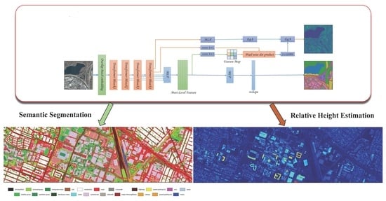
In this paper, we combine the relative height estimation task and semantic segmentation task into one task (as shown in Figure 1). We hope that this multi-task learning [39] can mutually promote in training, so an outcome better than the single task method can emerge. Experiments show that our method is superior to the recent multi-task learning and is significantly smaller than other models in parameter quantity. In summary, the main contributions of this paper are as follows:
  • We change the relative height estimation in multi-task learning from a regression task to a classification task and the whole multi-task learning into a classification task to better balance the tasks.
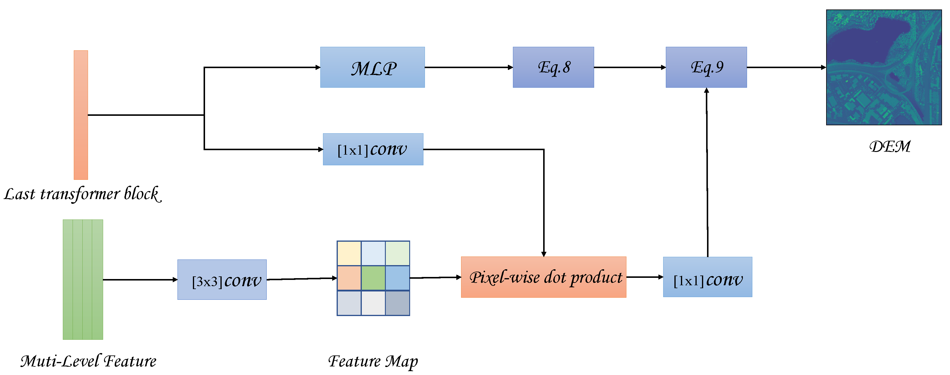
  • A unified architecture to realize semantic segmentation and relative height estimation. Our backbone uses a pure transformer structure, and only a small amount of convolution and MLP layers are used in the Segmentation module and Depth module (Figure 1).
  • In the relative height estimation module, we transform the original continuous value regression into ordinal number regression.
  • The whole neural network adopts an end-to-end structure, and only pairs of images are required for training.

2. Related Works

There are many applications in remote sensing to extract information from related regions using multi-source data. It is expensive to obtain 3D data from corresponding regions using information captured directly by sensors. At the same time, extracting depth information from a single image has received wide attention, and some research has been carried out (see Section 2.1). Therefore, it can be extended to the field of remote sensing to infer relative height from a single image (see Section 2.3). In order to combine multi-source data to obtain better model performance, we introduce semantic segmentation to assist relatively high inference (see Section 2.2). Finally, we briefly review the previous multi-task learning methods (see Section 2.4).

2.1. Monocular Depth Estimation from Images

Depth estimation is an important branch of computer vision and a tool for understanding three-dimensional scenes from images. In the traditional methods of monocular depth estimation, the model is mainly based on the inherent feature information of the images, such as hidden points [40], shadows [41], and focus and defocus [42], to complete the mapping relationship between pixels and depth values in the image. Although these methods have achieved some results in specific scenarios, additional assumptions about depth estimation are required. With the development of computer vision, researchers have proposed a variety of artificial design feature extractors, including SIFT [43] (scale-invariant feature transform), SURF [44] (scale-invariant feature transform), and so on. Considering the limitations of the artificially designed feature selector, researchers attempt to construct CRF (conditional random field) or Markov random field equal probability map models using the artificial feature extractor. The estimation problem is transformed into a learning problem under the random field by introducing global information into the calculation.
The rapid development of deep learning drives the model automatically to mine the information of the image stratum in a data-driven way, and its performance in image classification, target detection, and other fields is much better than that of traditional methods. Eigen et al. [38] rely on a mapping relationship between image pixel values and depth values, use deep learning to estimate monocular depth using a regression for the first time, and have achieved preliminary experimental results. Lee et al. [45] implemented monocular depth estimation from a frequency domain perspective by introducing a Fourier transform help network. Liu et al. [46] introduced a conditional random field into the convolution neural network to estimate depth information in the image. Xu et al. [47] proposed a sequence depth network framework with a multiscale Association CRFs structure and designed a C-MF module to extract multiscale information by stacking the module continuously. The multiscale information is fused in the decoder. With the advent of the attention mechanism, Xu et al. [48] proposed a multiscale CRFs model of structured attention mechanism. By introducing an attention mechanism, information transfer between different scale features can be automatically adjusted to improve depth estimation accuracy.

2.2. Semantic Segmentation

Semantic segmentation [49] as one of the three core tasks in the field of computer vision is a combination of image classification, object detection, and image segmentation. Through specific methods, image segmentation into a particular semantic meaning of a regional block, block and identify each area of the semantic category, realize the semantic reasoning process from bottom to top, and eventually obtain a picture with per-pixel semantic annotation of image segmentation. For the current field of semantic segmentation, most methods have the following paradigm, as shown in Figure 2.

2.3. Relative Height/Depth Estimation

The previous methods for extracting relative height are divided into photogrammetry based on stereo pairs, structure from motion, and lidar-based methods. These methods can provide high-resolution relative height, but in the extraction process, a lot of pre- and post-processing is required, including accurate denoising of input data. In addition, these methods are expensive and require solid professional knowledge and high computing power. However, thanks to the rapid development of deep learning and robust neural network models, relative height estimation using a single image has become popular. In computer vision, monocular depth estimation is a classic problem in many applications. Our task can be simply analogous to monocular depth estimation [38,50] in the field of computer vision. Monocular depth estimation is a crucial technology for understanding the geometric information of 3D scenes, but is also a pathological problem. Most methods to study monocular depth estimation extract the hierarchical features of images through DCNN, solve the problem by regression, and update the model parameters by designing the loss function of the minimum mean-square error. For traditional depth estimation networks, most of the structures adopted are shown in Figure 3a.
As shown in Figure 3a, monocular depth estimation uses a neural network structure similar to U-Net [49]. Encoder continuously reduces the size of the feature map by using convolution operation. However, for the final decoder to generate a depth map with more low-level and high-level information about the original image, it uses jump connection and other operations. In the whole neural network structure, the basic characteristics of convolution are utilized to obtain a larger receptive field by reducing the size of the feature graph so that more global information can be obtained in the deeper layers of the network. In contrast, more local information can be obtained in the shallow layers. For the decoder, local feature information and global feature information extracted by Encoder are used to increase the size of the feature graph step by step through deconvolution, and finally, mean-square error loss is constructed with a real depth map to realize model parameter updates. The model loss function is as follows:
L L 2 y ˜ , y = 1 H W i = 0 H 1 j = 0 W 1 y i j y ˜ i j 2
In recent years, there has been relatively little work on relative height estimation using neural networks in the field of remote sensing. At present, the relative height estimation in remote sensing can be roughly divided into two categories: the first is to generate the relative height of the corresponding region based on GAN (Generative Adversarial Network), and the second is to estimate the relative height based on regression. Panagiotou et al. [18], and Ghamisi et al. [51] proved that the relative height of the corresponding region can be estimated by using CGAN [52]. However, because the antagonism learning itself only focuses on the similarity between images, the model effect is relatively general. For GAN [36], the model structure consists mainly of generators and discriminators. The generator receives random noise through which the image is generated. For discriminators, the primary function is to determine whether a photo is real or not. The input of the discriminator is a picture, and 0 or 1 is the output through the discriminator. In the whole training process of the network, the goal of the generative network is to generate as many real pictures as possible to deceive the discriminator, and the discriminator’s goal is to distinguish the pictures generated by the generator from the real pictures as much as possible. From a macro view, the generator and discriminator constitute a dynamic game process. In the whole training process, the objective function is as follows:
min G max D V D , G = E x p d a t a x l o g D ( x ) + E z p z z l o g 1 D G z
where x represents the real picture, z represents the random noise of the input generator G, G(z) represents the picture generated by the generative network, and D represents the discriminator. D(x) represents the probability that the network will judge whether the picture is accurate. If true, the discriminated output should be as close to 1 as possible.
Regarding CGAN, it is an improvement on GAN. The conditional generation model is realized by adding additional condition information, such as category label, to the generator and discriminator of the original GAN. Compared with GAN, CGAN has a slight improvement in the objective function, and the specific formula is as follows:
min G max D V D , G = E x p d a t a x l o g D ( x | y ) + E z p z z l o g 1 D G z | y
As shown in Figure 3b, in CGAN, we can achieve image translation, style conversion, and other feats that the original GAN cannot by changing the condition information.
Because GAN-based relative height estimation has significant errors and there are many hyperparameters in training, Ghamisi et al. [51], Amirkolaee et al. [53], Liu et al. [54] and Li et al. [55] use a regression-based method to achieve relative height estimation, and the experimental results are better than those based on GAN. It is worth noting that the relative height referred to here is nDSM (normalization DSM), which is obtained by subtracting DEM from DSM in the corresponding area. For nDSM, the height information of terrain is ignored, and only the height of objects is concerned.

2.4. Multi-Task Learning

At present, many machine learning tasks are based on single-task learning. Complex tasks can be divided into multiple simple and independent sub-tasks to solve independently and then combine the results to obtain the solution of the initial complex task. However, many tasks seem to be very complex, and it is challenging to split each independent sub-task. Even if they can be divided, each sub-task is related to each other, linked by some shared parameters or shared representation. This approach ignores the rich association information between tasks. For multi-task learning [56,57], multiple related tasks are learned simultaneously, and some information is shared between multiple tasks to obtain better generalization ability than single-task learning. From Figure 4, we can find the difference between multi-task and single-task learning.
From the perspective of methodology, the current mainstream multi-task learning can be divided into Hard Parameter Sharing and Soft Parameter Sharing, as shown in Figure 5. For hard parameter sharing, the model shares some parameters among all tasks and uses its unique parameters in particular tasks. Obviously, in this model, the model is challenging to fit, and the sharing layer of the entire network tends to learn feature representation that is better for all tasks. For soft parameter sharing, each task has its parameters. Finally, the overall multi-task learning can be carried out by combining the differences between the parameters of different tasks. Compared with hard parameter sharing, soft parameter sharing has the following advantages:
  • Implicit Data Augmentation: In multi-task learning, sample noise exists in each task, and the noise is different among tasks, which can be partially canceled out by multi-task learning.
  • Help Feature Learning: Some features may be challenging to learn in the main task but can be well learned in the auxiliary task. This way, the auxiliary task can be designed to learn these features.
Up to now, there are many studies on multi-task learning. Liebel et al. [58], and Mobarakol et al. [59] have proved that combining multiple tasks to form a multi-task learning model is effective for each single task learning, and will also help the model converge faster. From the perspective of knowledge transfer, Rostami et al. [60] constructed task descriptors to describe the degree of correlation between tasks, further helping the model better learn the relationship between multiple tasks as to optimize the task performance. In autonomous driving, Song et al. [61] used the left and right images of binocular cameras and constructed a multi-task learning model to complete end-to-end depth estimation and semantic segmentation.
In remote sensing, Srivastava et al. [62] combined semantic segmentation and nDSM (normalization DSM) prediction of the corresponding region to build a multi-task learning network. In this structure, multiple tasks share a backbone network and finally use the full connection layer to realize task decoupling. The multi-task architecture proposed by Carvalho et al. [63] tends to split between two task-specific branches. For tasks such as semantic mapping and nDSM regression, the model effect is much better than the previous multi-task model. Benjamin et al. [64] used a single aerial image to construct a multi-task learning model to complete regional semantic segmentation and distance estimation. Experiments show that the introduction of multi-task learning can effectively help segment tasks. Compared with these, our multi-task model hopes to use the category information of semantic segmentation to optimize the regression of nDSM, which is a more appropriate design pattern.

3. Method

3.1. Our Network Architecture

This section mainly introduces the multi-task neural network model we designed, as shown in Figure 6. We introduce the basic structure of our model step by step from the primary Transformer Encoder. Our model mainly consists of three main modules: (1) a multi-scale feature extraction module is used to extract features of different levels in images; (2) a Semantic segmentation module is used to realize the semantic segmentation sub-task; (3) a Relative height estimation module is used to realize the sub-task of relative height estimation.

3.1.1. Transformer Encoder

Unlike the original Vision Transformer [30], there is no position embedding in our Transformer structure [65], which limits the expansion capability of the Transformer. For semantic segmentation and relative height estimation, the input image size is not necessarily the same, so the addition of position embedding in training causes some limitations on image input for practical applications. In ViT, input an image and use convolution to divide it into multiple image blocks and flatten them into vectors. Since Transformer does not change the vector size, most work only uses the tokens of the last Transformer Encoder. Our work refers to the multi-scale feature fusion commonly used in CNN. In order to make better use of the output of each layer of the Transformer Encoder layer, there is a convolution layer before the input of the Transformer Encoder layer, which reduces the image resolution to half of the original.
The calculation formula for the original self-attention layer is as follows:
A t t e n t i o n Q , K , V = S o f t m a x Q K T d h e a d V
where Q , K , V have the same dimensions N × C , where N = H × W is the length of the sequence.

3.1.2. Layer Normalization

In computer vision, blindly stacked convolutional layers can not achieve better results than external networks and even bring adverse effects to model training, such as gradient disappearance and gradient explosion. For the problem of gradient disappearance, the residual structure proposed in ResNet better solved this problem, but for the problem of gradient explosion, the proposal of batchNorm was better solved. With Batch Normalization, the model can converge well, and the Batch Normalization does not change the position of the optimal solution in the hyperplane. Unlike Batch Normalization, Layer Normalization directly estimates the normalization statistics from the summed inputs to the neurons within a hidden layer, so the normalization does not introduce any new dependencies between training cases. This works well for RNNs and improves the training time and the generalization performance of several existing RNN models. More recently, it has been used in transformer models, and we have also used layer normalization after each of our transformer layer outputs, as follows:
μ l = 1 H i = 1 H x i l σ l = 1 H i = 1 H x i l μ l 2 y l = x l μ l σ l + ϵ γ + β
where H represents the number of hidden units in the layer, L represents the number of layers of the neural network, γ and β are learnable affine transformation parameters.

3.1.3. Multi-Scale Feature Extractor

Most previous Relative Height Estimation, Semantic Segmentation, and Multi-task learning models use the standard CNN architecture to extract features. Because the CNN architecture often includes some pooling layers, these pooling layers can use the output of different pooling layers to form multi-scale feature representations. With the continuous application of the Transformer in the field of computer vision, it has been found that Transformer can obtain more image information than CNN. Currently, in multiple tasks, the neural network based on transformer structure performs better than the neural network based on CNN, and the neural network structure design does not need to be particularly complex.
Since the convolution layer can retain the image position information [66], combined with the above priorities, we design the feature extraction network, as shown in Figure 7.
As shown in Figure 7, before the image enters the transformer block, we first divide the image into small patches through convolution operation and then conduct the transformer encoder four times. It should be noted that after each transformer block, convolution compression is used to compress the feature image, and the size is 1/4 of the original size. Specifically, feature maps with overlapping convolutional layers are used as transformer encoder input to obtain multi-level features with 1/4, 1/8, 1/16, and 1/32 resolution of the original image. In addition, in order to integrate multi-scale information and produce better feature representation to downstream tasks, some remedial measures such as segmented refinement, skip connection, and multi-layer deconvolution network can be adopted. However, this not only requires additional computing and memory costs, but also complicates the network architecture and training process. According to the latest research on semantic segmentation (segformer/maskformer), we only retain skip connections. We input the output of the transformer block of each layer into an MLP layer. Finally, we splice the features of different scales to obtain multi-scale feature expression. At the same time, it can be observed that the calculation method of the attention mechanism only depends on the first dimension of Q and the second dimension of V. Based on this, we use the convolution layer to change the dimensions of K and V from N × C to N R × C , which further reduces the amount of computation of the backbone network.
In general, in our network structure, the use of convolution layer to reduce image resolution fundamentally reduces the computational complexity of Transformer from O n 2 to O n 2 N .

3.1.4. Semantic Segmentation Module

For the semantic segmentation module, we believe that the transformer block we designed can better obtain the feature expression of the image, so we use one MLP layer, then reshape to 1/4 of the edge length of the original image, and finally interpolate to the same size as the original image through bilinear interpolation [67], as shown in Figure 8.
As shown in Figure 8, we input the features of transformer encoders in different layers into the MLP layer. In detail, for the MLP layer, we first adjust the dimensions of features of different scales through a linear layer and then splice these unique arrays together and input them into a convolution layer to realize semantic segmentation. It is worth noting that the size of the output characteristic graph of our last convolution layer is only 1/4 of the side length of the original graph. We obtain a characteristic graph of the same size as the original graph through bilinear interpolation.

3.1.5. Relative Height Estimation Module

In computer vision, monocular depth estimation represents a classic problem essential in many applications. Inspired by recent studies on monocular depth estimation [50], we believe that relative height estimation can also be analogous to special monocular depth estimation.
In our paper, inspired by Adabins [68], we transform the depth estimation problem from regression to a classification problem, which is beneficial for us to perform semantic segmentation tasks simultaneously. In previous research on relative height and depth estimation, most of the problems were attributed to regression or generation problems, such as GAN [36,51]. For regression, the encoder–decoder structure is mostly used to make the model fit the actual data distribution as much as possible, as shown in Figure 6. However, this model generates depth or relative height with a more or less negligible ladder effect and therefore does not produce a more realistic looking depth map. As shown in Figure 9, we designed a method to use multi-level semantic information and feature information of the last layer to generate relative height.
In the Relative Height Estimation module, we use a few convolution layers to realize dimension transformation and feature compression and a pixel-level attention mechanism to realize relative height estimation finally.
MLP layer. In this part, the token output of the previous Transformer layer is mainly used for feature embedding before classification. In the MLP layer, we use the linear layer and LeakyReLU as the activation function, where the linear layer mainly implements feature expansion. For LeakyReLU, the formula is as follows:
L e a k y R e L U = x i f x 0 n e g a t i v e s l o p × x o t h e r w i s e
where n e g a t i v e s l o p is usually set to 0.01, LeakyReLU [69] solves the problem of neuron death in ReLU so that the gradient can also be calculated for the part of the LeakyReLU activation function input that is less than zero in the neural network backpropagation update, rather than the zero value of ReLU.
After passing through the MLP layer, we normalize the output vector bins so that their sum is 1, and the change formula is as follows:
b i n s i = b i n s i + ϵ j = 1 N b i n s j + ϵ
where ϵ = 10 3 . This design ensures that all bin widths are strictly a positive number, and regularizes the network to focus on how best to divide the depth interval.
Pixel-wise dot product. In the model structure, multi-scale feature maps represent high-resolution features, while transformer output embedding represents more global feature information. We use a 3 × 3 convolution layer for multi-scale features, which does not change the size of the feature maps but increases the area of the receptive field. For transformer output embedding, only 1 × 1 convolution layer is used to adjust the channel, and finally, a pixel-level attention mechanism is used to generate the attention map.
Model regression. A 1 × 1 convolution layer is used for the output attention attempt to achieve depth classification. As with previous classification tasks, after the 1 × 1 convolution layer, the Softmax function is used to obtain N channels. We obtained N softmax values b j through the previous MLP layer and Softmax function. We obtained the corresponding depth values of each interval center by using the previously set maximum depth and minimum depth values. The formula is as follows:
C b j = d e p t h m i n + d e p t h m a x d e p t h m i n × b i 2 + j = 1 i 1 b j
Finally, the pixel-level characteristic information and the depth of the interval center obtained from the previous attention diagram are used to obtain the final depth value, and the formula is as follows:
d e e p = k = 1 N C b k p k

3.2. Loss Function

Relative Height Estimation Loss. In our experimental design, we refer to the loss function design of original Adabins. Specifically, the loss function includes Pixel-wise depth loss and bin-Center Density Loss. For Pixel-wise depth loss [38], the specific formula is as follows:
L p i x e l l o s s = α 1 T i g i 2 λ T 2 i g i 2
where g i = log d ˜ i l o g   d i and ground true depth d i and T denotes the number of pixels having valid ground true values. We use λ = 0.85 and α = 10 for all our experiments.
For bin-center Density Loss, we hope that the Bin distribution divided automatically by our model is roughly similar to the distribution in the actual image. Here, we define C b i as the center depth of the ith Bin, GT represents the depth value of the actual image, and introduce Chamfer Loss into the loss function:
L b i n = c h a m f e r G T i , c b i + c h a m f e r c b i , G T i
Meanwhile, to make the relative height output from the Relative Height Estimation module similar to the real relative height structure, a structural similarity index (SSIM) is introduced to calculate the similarity of the two images. The specific formula is as follows:
L X , Y = 2 μ X μ Y + C 1 μ X 2 + μ Y 2 + C 1 C X , Y = 2 σ X σ Y + C 2 σ X 2 + σ Y 2 + C 2 S X , Y = σ X Y + C 3 σ X σ Y + C 3 S S I M = L X , Y × C ( X , Y ) × S X , Y
For SSIM, if two images are exactly the same, then S S I M = 1, so design L S S I M as follows:
L S S I M = 1 S S I M
Finally, the loss function of relative height estimation is defined as:
L r e l a t i v e h e i g h t = L p i x e l l o s s + α L S S I M + β L b i n
where α and β are the hyperparameters, we define. In the experiment, the hyperparameter can be set as a learnable parameter, but due to the slow convergence, we set them to 0.1 in our experiment.
Semantic Segmentation Loss. We simply define the semantic segmentation task as a pixel-level classification task for the loss function. For the semantic segmentation task, the optimization function is as follows:
min i c l a s s e s y P r e d l o g p P r e d
where y P r e d is a one-hot vector. The elements in the vector have only two values: 0 and 1. If the predicted category is the same as the actual category, the corresponding position is 1, p P r e d is the probability that the corresponding pixel belongs to i.

3.3. Multi-Task Learning Strategy

For multi-task learning, a primary research focus is learning how to balance multi-tasking. If there is no well-defined balance of multi-tasking, then the neural network can complete a relatively simple task to achieve the global optimal. However, multi-tasking between simple artificial weights of linear weight is insufficiently accurate and inconvenient. So most of the work on the loss magnitude of the multi-tasking loss function is optimized, including GradNorm which considers the magnitude of loss and the training speed of different tasks. However, every step in the training model iteration needs significant additional gradient calculation when the weight function parameters increase, which will significantly influence the training speed. Therefore, we refer to the design method of GradNorm [70] and MTAN [71] to design the weight parameters of the loss function, which only needs to consider the current loss and the loss of the last iteration. The specific calculation method is shown in Algorithm 1.
Algorithm 1 Weight dynamic adjustment algorithm for Multi-task training loss function
1:
for each iteration [ 1 , 3 ]  do
2:
      initialize lambda weight using a constant
3:
      for each task [ 1 , m ]  do
4:
          lambdatask = 1;
5:
    end for
6:
end for
7:
foriteration = 4 to n do
8:
      calculate lost momentum;
9:
      momentumtask = l o s s t a s k i t e r a t i o n l o s s t a s k i t e r a t i o n 1
10:
    calculate the weight of different task loss functions;
11:
    lambdtask = e m o m e n t u m t a s k / T i t a s k s e m o m e n t u m i / T
12:
    Multi-task loss function;
13:
     L o s s t o t a l = l a m b d a s e g × L o s s s e g + l a m b d a r e l a t i v e h e i g h t × L o s s r e l a t i v e h e i g h t
14:
end for

3.4. Differences and Limitations Compared to Other Studies

We directly convert the original relative height estimation tasks into classification tasks compared with previous relative height estimation studies. At the same time, our model design is more straightforward, and there is no need to stack many network layers to achieve feature extraction. For our multitask learning model design, considering that the previous multitask learning network did not make good use of the category information obtained by semantic segmentation, we integrate the category information of semantic segmentation into the relative height estimation in the network design, which can assist information exchange between multitasks.
In our multi-task learning strategy, we do not consider the gradient in the loss function compared to other methods such as GradNorm [70]. The benefit is that the network does not need to introduce additional computational effort in training. However, it may bring some limitations to the network, i.e., the optimal balance may not be achieved between tasks.

4. Experiment

4.1. Dataset

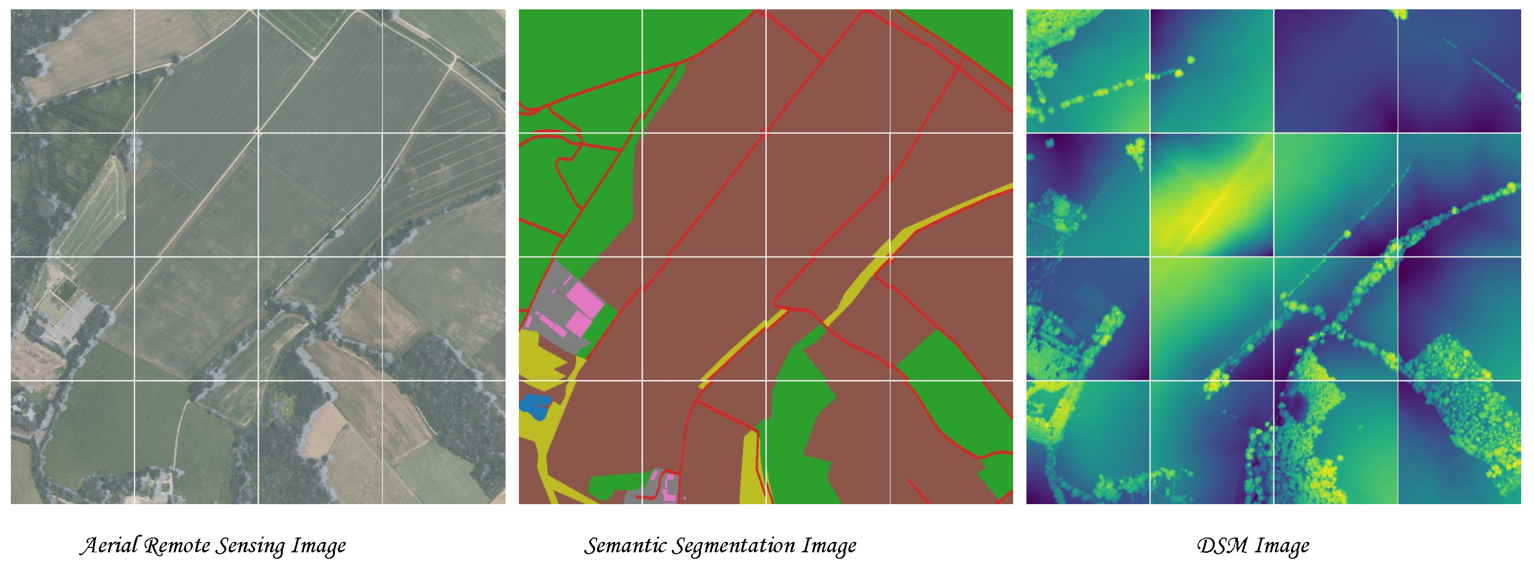
GeoNRW [72]. We use the high-resolution remote sensing dataset GeoNRW to verify the effectiveness of our method. The dataset includes remote sensing satellite images, semantic segmentation images, and DSM images, and the relationship between them is a one-to-one correspondence. See Figure 10 for the distribution of feature types in the dataset. For DSM images, we change the minimum value of each image to 0, converting the original DSM to relative height [53].
The dataset includes orthophoto-corrected aerial photos, light detection and ranging (LIDAR)-derived DSM and 10 types of land cover maps from the German state of North-Rhine Westphalia. The pre-processing of the dataset includes downsampling the orthophoto-corrected aerial photos with a resolution of 10 cm to 1 m, which conveniently keeps the aerial remote sensing image and DSM image at the exact resolution. In our experiments, we found that there are partial annotation problems in the semantic segmentation of the dataset, including the inaccurate classification of objects and more than 10 categories.
Through statistical analysis of ground types, the following problems exist in the distribution of original data:
  • There are obvious problems of unbalanced distribution in data distribution. Some categories have a large number, while others have a small number.
  • Through the examination of DSM distribution, we find that the DSM data distribution is too large, which increases the difficulty of DSM generation, and the transformation into relative elevation estimation will greatly reduce the task difficulty.
The first problem mentioned above is usually solved by directly weighing different types of losses in training. In our training, we also adopted this method. Specifically, for each category, the weight calculation formula is as follows:
W e i g h t i = 1 l o g 1.02 + f r e q i t o t a l
Before processing, we divided the original 1000 × 1000 image into 256 × 256 image with partial overlap, as shown in Figure 11.
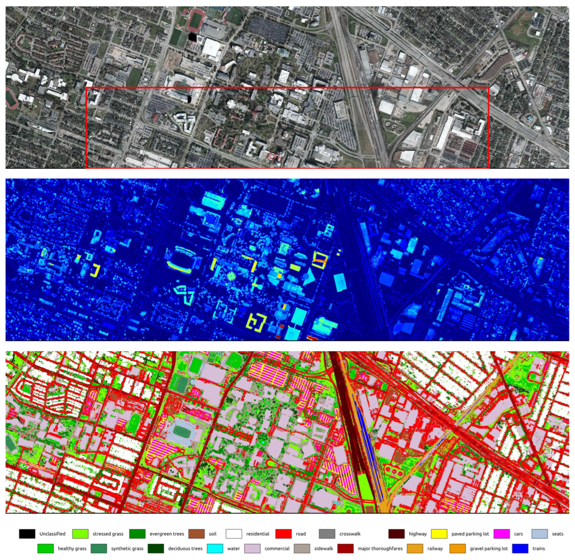
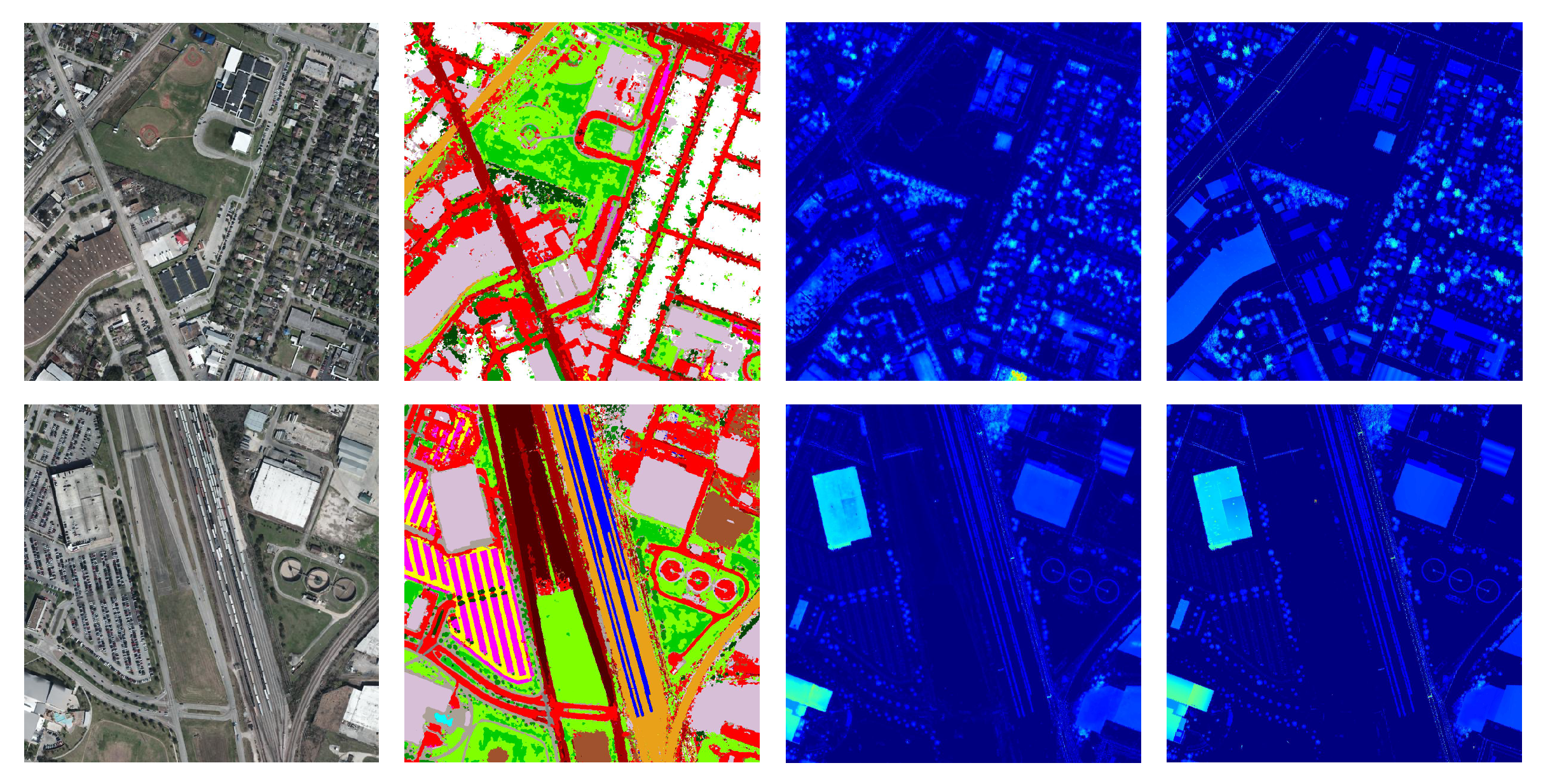
Data Fusion Contest 2018 (DFC2018) dataset [73]. The dataset is a collection of multisource optical images from Houston, Texas. The data include ultra-high resolution (VHR) color images resampled at 5 cm/pixel, hyperspectral images, and DSM and DEM obtained with lidar, particularly at 50 cm/pixel resolution. The original DCF2018 dataset does not contain a height map, so we use DSM minus DEM to obtain the height within the area. Figure 12 shows the distribution of the dataset.
The OSI dataset [54]. The dataset is an optical image set from Dublin, including the height obtained by lidar and the corresponding color image, with a 15 cm/pixel resolution. In particular, all data are collected by UAV, with a flight height of about 300 m and a total coverage area of 5.6 square kilometers.

4.2. Data Augmentation

Data augmentation is an indispensable step in deep learning image processing. It refers to performing transformation operations on the training sample data to generate new data. The fundamental purpose of data expansion is to provide more abundant training samples through image transformation, increase the robustness of the training model and avoid model over-fitting.
For our definition of the task, because remote sensing images are the data source, the imaging process of the sensor captures the same image objects of different points of view that will be displayed on the image of different locations and shapes. This can make model transformation after the sample much easier to understand regarding the characteristics of the rotating invariance, to better adapt to the different forms of the image. Therefore, we introduced geometric transformation in training, including horizontal and vertical flips.
Meanwhile, since we need to obtain relative height information from the image, there is no hard data augmentation for the image. Since relative height data are distributed in an extensive range, we must manually map relative height data. The specific formula is as follows:
R e l a t i v e H e i g h t = R e l a t i v e H e i g h t M i n R e l a t i v e H e i g h t
Through the above equation, we shift the minimum height value of each image to 0, which can help the model better learn the concept of relative height.

4.3. Network Training Strategy and Evaluation Metric

In deep learning experiments, warmup is usually added in training to prevent the model from fitting data too early, reducing the risk of over-fitting and improving the model’s expression ability. Warmup usually has 1–3 epochs at the beginning of training. In our experiment, we used 2000 iterations.
Evaluation Metric is divided into Pixel Accuracy, Mean Accuracy, Mean IoU (MIoU), test height Error ABS, test height Error REL, RMSE, MAE, and SSIM. Among them, the first three items are all evaluation indexes to measure semantic segmentation, and the last five are to measure relative height estimation accuracy. The calculation formula of each evaluation index is as follows:
P i x e l A c c u r a c y = N u m b e r p i x e l p r e d i c t t r u e N u m b e r p i x e l
M e a n A c c u r a c y = i c l a s s e s a c c u r c y i c l a s s e s
I o U = G T P r e d G T P r e d M I o U = i c l a s s e s I o U i c l a s s e s
M I o U = i c l a s s e s I o U i c l a s s e s
R e l a t i v e H e i g h t E r r o r A b s = i r o w s j c o l s H e i g h t P r e d i , j H e i g h t T r u e i , j
R e l a t i v e H e i g h t E r r o r R e l = i r o w s j c o l s H e i g h t P r e d i , j H e i g h t T r u e i , j H e i g h t P r e d i , j
R M S E = 1 n H e i g h t P r e d H e i g h t T r u e 2
M A E = 1 N H e i g h t P r e d H e i g h t T r u e
where G T represents the ground true value, P r e d represents the result of model prediction, H e i g h t P r e d and H e i g h t T r u e represent the true value of model prediction at i , j , μ X and μ Y are the mean values of X and Y, σ X and σ Y are the standard deviations of X and Y, C 1 , C 2 , and C 3 are constants, respectively.

4.4. Implementation Details

On the experimental platform, we used an AMD core R9-5900x 3.70 GHz 12 core processor with 32.0 GB memory (Micro DDR4 3200 mhz) and a Geforce RTX 3090 graphics card with 24 GB video memory. In terms of the software environment, we used the Ubuntu operating system. The programming language used is Python, and the deep learning framework used is PyTorch. For the design of experimental parameters, we design batchsize = 64, learning rate = 6 × 10⁻⁴, warm-up iterations = 2000, total iterations = 100,000, and we use AdamW optimization algorithm to accelerate the training of the model, where β = 0.9 , 0.999 , λ = 0.01 , ϵ = 1 × 10 8 . For more details, the code for our work will be available at https://github.com/Neroaway/Multi-Task-Learning-of-Relative-Height-Estimation-and-Semantic-Segmentation-from-Single-Airborne-RGB.

5. Results and Discussion

5.1. Comparative Experiments of Different Methods

In order to test the rationality and effectiveness of the experimental design, we employ MTAN [71], CycleGAN [74], and Pix2Pix [52] as the comparison method, in which CycleGAN and Pix2Pix are used for the comparison of relative height estimation, and MTAN is used as the comparison of multi-task learning. At the same time, we also test the performance of our model on a single task.
MTAN [71] is a multi-task learning algorithm based on an attention mechanism. It uses a backbone to share features and has its attention module for each task. The features extracted by backbone are returned to a single task through the attention module. The main contribution of this paper is to obtain more global feature information through the backbone and then use the attention module to obtain more useful feature information for a single task. The advantage is that when the model can be extended to n tasks, you only need to add the attention module.
Pix2Pix [52] is a generative model based on GAN, which is different from the original GAN. The input of the original GAN is randomly initialized Gaussian noise. In contrast, Pix2Pix directly inputs the image to be transformed into the network and uses the pairing relationship between pixels in the image to generate the image.
CycleGAN [74] is also a generative model based on GAN. The difference is that it does not need the strict pairwise relationship between images. It constructs the mapping relationship from set A to set B and from set B to set A. Its main contribution is to solve the requirements of solid data coupling in GAN, and the model effect is no less than Pix2Pix.
Meanwhile, we also compare the calculation amount, parameter amount, and the time required to infer an image.
According to Table 1 and Table 2, it can be found that the method designed by us is far better than similar current methods in terms of both computational amount and model effect. Moreover, the multi-task learning model we designed also outperforms single-task learning in model performance. Meanwhile, to further study the attention diagram of the network in the learning process, we use Grad-CAM to visualize the specificity of the last layer of our semantic segmentation.
In order to further verify the validity of our designed model, we performed multi-task and single-task experiments in the OSI Dataset [54] and DFC2018 Dataset [73], respectively. The current mainstream methods are compared, and the specific experimental results are shown in Table 3 and Table 4.

5.2. Prediction Results of Our Model on the DFC2018 Dataset

In this section, we visualize the model’s predictions, including the semantically segmented results and the relative height estimates. It is important to note that it is critical to be able to better infer a large map. To avoid the checkerboard effect, we use a Gaussian prior approach. We predict patches in step order smaller than the window size and use a 2D Gaussian map to weigh the overlapping areas. Here, we use a 512-pixel window and a 64-pixel step. The result is shown in Figure 13.
Meanwhile, we also visualized the reasoning results of each individual scenario, as shown in the following figure.
As you can see from Figure 14, our model demonstrates a good grasp of the structure information of buildings. At the same time, for information not captured at the original relative height, similar to the bulge of the roof, our model can also be captured sharply, which verifies the validity and robustness of our model.

5.3. Prediction Results of Our Model on the GeoNRW Dataset

As shown in Figure 15, our model can segment the feature categories well. Meanwhile, it can better understand which part of the model pays more attention to the input image. In the specific experiment, we use grad norm to visualize the degree of attention of our model to the agricultural region and visualize it. From the fourth line image in Figure 15, we find that our model can pay good attention to the agricultural area in the image and does not pay attention to other types of areas.
As shown in Figure 16, we visualized the output of the relative height estimation module. In Figure 16, it can be found that in different scenarios, our relative height estimation module can well generate the relative value of the ground.

5.4. Comparative Experiment of Different Bins Values

In our relative height estimation module design, the bin is a hyperparameter. We also compared the effects of setting different bins on the results to obtain the effects of the hyperparameter on the results. The following Table 5 shows the experimental results on the GeoNRW dataset.
As seen from Table 5, the number of bins settings has little influence on the experiment results. At the same time, the greater the number of bins settings, the smaller the actual error of relative height, but the number of network parameters is also more significant.

5.5. Comparative Experiment of Different Relative Height Loss Function

Three different loss functions are introduced in the design of the loss function of our relative height estimation module, including L p i x e l l o s s , L S S I M , and L b i n . We designed an ablative study to verify the impact of each loss term on the final performance. The following Table 6 shows the experimental results on the Dublin dataset.
As shown in Table 6, we can see that the model performs best when all loss function terms exist. It is also surprising that when only L S S I M is used for model training, the effect of the model does not decrease much. The ablation study shows that the loss function items designed by our experiment can effectively help the model achieve the lowest prediction error, and the relative height map predicted by the model has a high similarity with the accurate relative height map.

6. Conclusions

This paper proposes a novel multi-task learning model different from previous multi-task learning based on attention mechanisms. Based on the transformer, this paper uses multi-level semantic information and global information to carry out semantic segmentation and relative height estimation at the same time, and the whole model uses only a small amount of convolution structure, which makes the calculation and parameters of the whole model less than the previous methods. In order to balance the competition and network deviation in multi-task learning, we design a momentum method to measure the task’s difficulty and further determine the optimization direction of the network. The model was tested on three data sets, and its performance is significantly better than other state-of-the-art methods, and the reasoning speed is also significantly faster than other methods. The results show that the model can effectively model problems in related fields. Moreover, in order to further illustrate the rationality of the model design, we conducted a relevant ablation study for part of the loss function design.
For future work, there remain many avenues where our method can be further studied and explored. (1) Design a more reasonable multi-task model. Although our model has achieved good results, the relative height estimation module design can still be further explored. (2) A more reasonable multi-task learning balance method. In our model, we only consider the momentum lost by the model and do not balance multi-tasks from the perspective of the gradient. Methods to design a better multi-task learning balance model is the key to multi-task learning. (3) More reasonable loss function. Regarding the loss function, it helps the model better mine the information in the image. For multi-task, the loss function design can accelerate the model’s convergence and improve the model’s robustness. (4) More robust data enhancement. In our experiment, we only use the flip operation as to not affect the original image data distribution. For the deep learning model, data enhancement is key. Better data enhancement can make the model more robust and effective. The method proposed in this paper is simple and feasible, and the model performs far better than the other most advanced deep learning methods. In this method, the corresponding region’s classification result and relative height can be obtained using a single RGB image without other additional information. Compared with the traditional method of obtaining relative height, this method dramatically reduces the time and labor cost of data collection and the difficulties brought by subsequent complex data processing.

Author Contributions

M.L. and J.L. proposed the original idea. M.L. performed the experiments and wrote the manuscript. J.L. and Y.X. reviewed and edited the manuscript. M.L., J.L. and F.W. contributed to the direction, content, and revised the manuscript. All authors have read and agreed to the published version of the manuscript.

Funding

This work was supported in part by the National Natural Science Foundation of China under Grant 61901439, and in part by Key Research Program of Frontier Sciences, Chinese Academy of Science, under Grant ZDBS-LY-JSC036.

Conflicts of Interest

The authors declare no conflict of interest.

References

  1. Smith, M.J.; Clark, C.D. Methods for the visualization of digital elevation models for landform mapping. Earth Surf. Process. Landforms 2005, 30, 885–900. [Google Scholar] [CrossRef]
  2. Dobos, E.; Micheli, E.; Baumgardner, M.F.; Biehl, L.; Helt, T. Use of combined digital elevation model and satellite radiometric data for regional soil mapping. Geoderma 2000, 97, 367–391. [Google Scholar] [CrossRef]
  3. Martınez-Casasnovas, J.; Ramos, M.; Ribes-Dasi, M. Soil erosion caused by extreme rainfall events: Mapping and quantification in agricultural plots from very detailed digital elevation models. Geoderma 2002, 105, 125–140. [Google Scholar] [CrossRef]
  4. Wechsler, S. Uncertainties associated with digital elevation models for hydrologic applications: A review. Hydrol. Earth Syst. Sci. 2007, 11, 1481–1500. [Google Scholar] [CrossRef] [Green Version]
  5. Walker, J.P.; Willgoose, G.R. On the effect of digital elevation model accuracy on hydrology and geomorphology. Water Resour. Res. 1999, 35, 2259–2268. [Google Scholar] [CrossRef] [Green Version]
  6. Zhang, C.; Lin, H.; Chen, M.; Yang, L. Scale matching of multiscale digital elevation model (DEM) data and the Weather Research and Forecasting (WRF) model: A case study of meteorological simulation in Hong Kong. Arab. J. Geosci. 2014, 7, 2215–2223. [Google Scholar] [CrossRef]
  7. Onorati, G.; Ventura, R.; Poscolieri, M.; Chiarini, V.; Crucilla, U. The digital elevation model of Italy for geomorphology and structural geology. Catena 1992, 19, 147–178. [Google Scholar] [CrossRef]
  8. Thompson, J.A.; Bell, J.C.; Butler, C.A. Digital elevation model resolution: Effects on terrain attribute calculation and quantitative soil-landscape modeling. Geoderma 2001, 100, 67–89. [Google Scholar] [CrossRef]
  9. Zhou, S.; Mi, L.; Chen, H.; Geng, Y. Building detection in Digital surface model. In Proceedings of the IEEE International Conference on Imaging Systems and Techniques (IST), Beijing, China, 22–23 October 2013; pp. 194–199. [Google Scholar]
  10. Dawid, W.; Pokonieczny, K. Analysis of the Possibilities of Using Different Resolution Digital Elevation Models in the Study of Microrelief on the Example of Terrain Passability. Remote Sens. 2020, 12, 4146. [Google Scholar] [CrossRef]
  11. Štular, B.; Lozić, E.; Eichert, S. Airborne LiDAR-derived digital elevation model for archaeology. Remote Sens. 2021, 13, 1855. [Google Scholar] [CrossRef]
  12. Shabou, A.; Baselice, F.; Ferraioli, G. Urban digital elevation model reconstruction using very high resolution multichannel InSAR data. IEEE Trans. Geosci. Remote Sens. 2012, 50, 4748–4758. [Google Scholar] [CrossRef]
  13. Luo, H.; Li, Z.; Dong, Z.; Liu, P.; Wang, C.; Song, J. A new baseline linear combination algorithm for generating urban digital elevation models with multitemporal InSAR observations. IEEE Trans. Geosci. Remote Sens. 2019, 58, 1120–1133. [Google Scholar] [CrossRef] [Green Version]
  14. Shean, D.E.; Alexandrov, O.; Moratto, Z.M.; Smith, B.E.; Joughin, I.R.; Porter, C.; Morin, P. An automated, open-source pipeline for mass production of digital elevation models (DEMs) from very-high-resolution commercial stereo satellite imagery. ISPRS J. Photogramm. Remote Sens. 2016, 116, 101–117. [Google Scholar] [CrossRef] [Green Version]
  15. Lee, H.Y.; Kim, T.; Park, W.; Lee, H.K. Extraction of digital elevation models from satellite stereo images through stereo matching based on epipolarity and scene geometry. Image Vis. Comput. 2003, 21, 789–796. [Google Scholar] [CrossRef]
  16. James, M.; Robson, S. Sequential digital elevation models of active lava flows from ground-based stereo time-lapse imagery. ISPRS J. Photogramm. Remote Sens. 2014, 97, 160–170. [Google Scholar] [CrossRef]
  17. Yu, H.; Yang, Z.; Tan, L.; Wang, Y.; Sun, W.; Sun, M.; Tang, Y. Methods and datasets on semantic segmentation: A review. Neurocomputing 2018, 304, 82–103. [Google Scholar] [CrossRef]
  18. Panagiotou, E.; Chochlakis, G.; Grammatikopoulos, L.; Charou, E. Generating Elevation Surface from a Single RGB Remotely Sensed Image Using Deep Learning. Remote Sens. 2020, 12, 2002. [Google Scholar] [CrossRef]
  19. Russell, S.; Norvig, P. Artificial Intelligence: A Modern Approach; Pearson Education, Inc.: London, UK, 2002. [Google Scholar]
  20. Voulodimos, A.; Doulamis, N.; Doulamis, A.; Protopapadakis, E. Deep learning for computer vision: A brief review. Comput. Intell. Neurosci. 2018, 2018, 7068349. [Google Scholar] [CrossRef]
  21. Forsyth, D.; Ponce, J. Computer Vision: A modern Approach.; Prentice hall: Hoboken, NJ, USA, 2011. [Google Scholar]
  22. Chowdhary, K. Natural language processing. Fundam. Artif. Intell. 2020, 603–649. [Google Scholar]
  23. Nadkarni, P.M.; Ohno-Machado, L.; Chapman, W.W. Natural language processing: An introduction. J. Am. Med. Inform. Assoc. 2011, 18, 544–551. [Google Scholar] [CrossRef] [Green Version]
  24. Haeb-Umbach, R.; Watanabe, S.; Nakatani, T.; Bacchiani, M.; Hoffmeister, B.; Seltzer, M.L.; Zen, H.; Souden, M. Speech processing for digital home assistants: Combining signal processing with deep-learning techniques. IEEE Signal Process. Mag. 2019, 36, 111–124. [Google Scholar] [CrossRef]
  25. Yu, D.; Hinton, G.; Morgan, N.; Chien, J.T.; Sagayama, S. Introduction to the special section on deep learning for speech and language processing. IEEE Trans. Audio Speech Lang. Process. 2011, 20, 4–6. [Google Scholar] [CrossRef]
  26. Deng, J.; Dong, W.; Socher, R.; Li, L.J.; Li, K.; Fei-Fei, L. Imagenet: A large-scale hierarchical image database. In Proceedings of the Conference on Computer Vision and Pattern Recognition, Miami, FL, USA, 20–25 June 2009; pp. 248–255. [Google Scholar]
  27. Krizhevsky, A.; Sutskever, I.; Hinton, G.E. Imagenet classification with deep convolutional neural networks. Adv. Neural Inf. Process. Syst. 2012, 25, 1097–1105. [Google Scholar] [CrossRef]
  28. Long, J.; Shelhamer, E.; Darrell, T. Fully convolutional networks for semantic segmentation. In Proceedings of the IEEE Conference on Computer Vision and Pattern Recognition, Boston, MA, USA, 7–12 June 2015; pp. 3431–3440. [Google Scholar]
  29. He, K.; Gkioxari, G.; Dollár, P.; Girshick, R. Mask r-cnn. In Proceedings of the IEEE International Conference on Computer Vision, Venice, Italy, 22–29 October 2017; pp. 2961–2969. [Google Scholar]
  30. Dosovitskiy, A.; Beyer, L.; Kolesnikov, A.; Weissenborn, D.; Zhai, X.; Unterthiner, T.; Dehghani, M.; Minderer, M.; Heigold, G.; Gelly, S.; et al. An image is worth 16x16 words: Transformers for image recognition at scale. arXiv 2020, arXiv:2010.11929. [Google Scholar]
  31. Revaud, J.; Weinzaepfel, P.; Harchaoui, Z.; Schmid, C. Deepmatching: Hierarchical deformable dense matching. Int. J. Comput. Vis. 2016, 120, 300–323. [Google Scholar] [CrossRef] [Green Version]
  32. Eiumnoh, A.; Shrestha, R.P. Application of DEM data to Landsat image classification: Evaluation in a tropical wet-dry landscape of Thailand. Photogramm. Eng. Remote Sens. 2000, 66, 297–304. [Google Scholar]
  33. Bahadur, K. Improving Landsat and IRS image classification: Evaluation of unsupervised and supervised classification through band ratios and DEM in a mountainous landscape in Nepal. Remote Sens. 2009, 1, 1257–1272. [Google Scholar] [CrossRef] [Green Version]
  34. Zhang, Y.; Yu, W. Comparison of DEM Super-Resolution Methods Based on Interpolation and Neural Networks. Sensors 2022, 22, 745. [Google Scholar] [CrossRef]
  35. Zhou, A.; Chen, Y.; Wilson, J.P.; Su, H.; Xiong, Z.; Cheng, Q. An Enhanced Double-Filter Deep Residual Neural Network for Generating Super Resolution DEMs. Remote Sens. 2021, 13, 3089. [Google Scholar] [CrossRef]
  36. Goodfellow, I.; Pouget-Abadie, J.; Mirza, M.; Xu, B.; Warde-Farley, D.; Ozair, S.; Courville, A.; Bengio, Y. Generative adversarial nets. arXiv 2014, arXiv:1406.2661. [Google Scholar]
  37. Kipf, T.N.; Welling, M. Variational graph auto-encoders. arXiv 2016, arXiv:1611.07308. [Google Scholar]
  38. Eigen, D.; Puhrsch, C.; Fergus, R. Depth map prediction from a single image using a multi-scale deep network. arXiv 2014, arXiv:1406.2283. [Google Scholar]
  39. Caruana, R. Multitask learning. Mach. Learn. 1997, 28, 41–75. [Google Scholar] [CrossRef]
  40. Tsai, Y.M.; Chang, Y.L.; Chen, L.G. Block-based vanishing line and vanishing point detection for 3D scene reconstruction. In Proceedings of the International Symposium on Intelligent Signal Processing and Communications, Yonago, Japan, 12–15 December 2006; pp. 586–589. [Google Scholar]
  41. Prados, E.; Faugeras, O. Shape from shading. In Handbook of Mathematical Models in Computer Vision; Springer: Berlin/Heidelberg, Germany, 2006; pp. 375–388. [Google Scholar]
  42. Tang, C.; Hou, C.; Song, Z. Depth recovery and refinement from a single image using defocus cues. J. Mod. Opt. 2015, 62, 441–448. [Google Scholar] [CrossRef]
  43. Lowe, D.G. Object recognition from local scale-invariant features. In Proceedings of the Seventh IEEE International Conference on Computer Vision, Kerkyra, Greece, 20–27 September 1999; Volume 2, pp. 1150–1157. [Google Scholar]
  44. Bay, H.; Tuytelaars, T.; Gool, L.V. Surf: Speeded up robust features. In Proceedings of the European Conference on Computer Vision, Graz, Austria, 7–13 May 2006; Springer: Berlin/Heidelberg, Germany, 2006; pp. 404–417. [Google Scholar]
  45. Lee, J.H.; Heo, M.; Kim, K.R.; Kim, C.S. Single-image depth estimation based on fourier domain analysis. In Proceedings of the IEEE Conference on Computer Vision and Pattern Recognition, Salt Lake City, UT, USA, 18–22 June 2018; pp. 330–339. [Google Scholar]
  46. Liu, F.; Shen, C.; Lin, G. Deep convolutional neural fields for depth estimation from a single image. In Proceedings of the IEEE Conference on Computer Vision and Pattern Recognition, Boston, MA, USA, 7–12 June 2015; pp. 5162–5170. [Google Scholar]
  47. Xu, D.; Ricci, E.; Ouyang, W.; Wang, X.; Sebe, N. Multi-Scale Continuous Crfs as Sequential Deep Networks for Monocular Depth Estimation. In Proceedings of the IEEE Conference on Computer Vision and Pattern Recognition, Honolulu, HI, USA, 21–26 July 2017; pp. 5354–5362. [Google Scholar]
  48. Xu, D.; Wang, W.; Tang, H.; Liu, H.; Sebe, N.; Ricci, E. Structured attention guided convolutional neural fields for monocular depth estimation. In Proceedings of the IEEE Conference on Computer Vision and Pattern Recognition, Salt Lake City, UT, USA, 18–23 June 2018; pp. 3917–3925. [Google Scholar]
  49. Ronneberger, O.; Fischer, P.; Brox, T. U-net: Convolutional networks for biomedical image segmentation. In Proceedings of the International Conference on Medical Image Computing and Computer-Assisted Intervention, Munich, Germany, 5–9 October 2015; Springer: Berlin/Heidelberg, Germany, 2015; pp. 234–241. [Google Scholar]
  50. Fu, H.; Gong, M.; Wang, C.; Batmanghelich, K.; Tao, D. Deep ordinal regression network for monocular depth estimation. In Proceedings of the IEEE Conference on Computer Vision and Pattern Recognition, Salt Lake City, UT, USA, 18–23 June 2018; pp. 2002–2011. [Google Scholar]
  51. Ghamisi, P.; Yokoya, N. IMG2DSM: Height simulation from single imagery using conditional generative adversarial net. IEEE Geosci. Remote Sens. Lett. 2018, 15, 794–798. [Google Scholar] [CrossRef]
  52. Isola, P.; Zhu, J.Y.; Zhou, T.; Efros, A.A. Image-to-image translation with conditional adversarial networks. In Proceedings of the IEEE Conference on Computer Vision and Pattern Recognition, Honolulu, HI, USA, 21–26 July 2017; pp. 1125–1134. [Google Scholar]
  53. Amirkolaee, H.A.; Arefi, H. Height estimation from single aerial images using a deep convolutional encoder-decoder network. ISPRS J. Photogramm. Remote Sens. 2019, 149, 50–66. [Google Scholar] [CrossRef]
  54. Liu, C.J.; Krylov, V.A.; Kane, P.; Kavanagh, G.; Dahyot, R. IM2ELEVATION: Building height estimation from single-view aerial imagery. Remote Sens. 2020, 12, 2719. [Google Scholar] [CrossRef]
  55. Li, X.; Wang, M.; Fang, Y. Height estimation from single aerial images using a deep ordinal regression network. arXiv 2020, arXiv:2006.02801. [Google Scholar] [CrossRef]
  56. Zhang, Y.; Yang, Q. A survey on multi-task learning. IEEE Trans. Knowl. Data Eng. 2021. [Google Scholar] [CrossRef]
  57. Zhang, Y.; Yang, Q. An overview of multi-task learning. Natl. Sci. Rev. 2018, 5, 30–43. [Google Scholar] [CrossRef] [Green Version]
  58. Liebel, L.; Körner, M. Auxiliary tasks in multi-task learning. arXiv 2018, arXiv:1805.06334. [Google Scholar]
  59. Islam, M.; Vibashan, V.; Ren, H. Ap-mtl: Attention pruned multi-task learning model for real-time instrument detection and segmentation in robot-assisted surgery. In Proceedings of the IEEE International Conference on Robotics and Automation (ICRA), 31 May–31 August 2020; pp. 8433–8439. [Google Scholar]
  60. Rostami, M.; Isele, D.; Eaton, E. Using task descriptions in lifelong machine learning for improved performance and zero-shot transfer. J. Artif. Intell. Res. 2020, 67, 673–704. [Google Scholar] [CrossRef]
  61. Song, T.J.; Jeong, J.; Kim, J.H. End-to-End Real-Time Obstacle Detection Network for Safe Self-Driving via Multi-Task Learning. IEEE Trans. on Intell. Transp. Syst. 2022, 1–12. [Google Scholar] [CrossRef]
  62. Srivastava, S.; Volpi, M.; Tuia, D. Joint height estimation and semantic labeling of monocular aerial images with CNNs. In Proceedings of the IEEE International Geoscience and Remote Sensing Symposium (IGARSS), Worth, TX, USA, 23–28 July 2017; pp. 5173–5176. [Google Scholar]
  63. Carvalho, M.; Le Saux, B.; Trouvé-Peloux, P.; Champagnat, F.; Almansa, A. Multitask learning of height and semantics from aerial images. IEEE Geosci. Remote Sens. Lett. 2019, 17, 1391–1395. [Google Scholar] [CrossRef] [Green Version]
  64. Bischke, B.; Helber, P.; Folz, J.; Borth, D.; Dengel, A. Multi-task learning for segmentation of building footprints with deep neural networks. In Proceedings of the IEEE International Conference on Image Processing (ICIP), Taipei, Taiwan, 22–25 September 2019; pp. 1480–1484. [Google Scholar]
  65. Vaswani, A.; Shazeer, N.; Parmar, N.; Uszkoreit, J.; Jones, L.; Gomez, A.N.; Kaiser, Ł.; Polosukhin, I. Attention is all you need. Adv. Neural Inf. Process. Syst. 2017, 30, 6000–6010. [Google Scholar]
  66. Xie, E.; Wang, W.; Yu, Z.; Anandkumar, A.; Alvarez, J.M.; Luo, P. SegFormer: Simple and efficient design for semantic segmentation with transformers. Adv. Neural Inf. Process. Syst. 2021, 34, 12077–12090. [Google Scholar]
  67. Kirkland, E.J. Bilinear interpolation. In Advanced Computing in Electron Microscopy; Springer: Berlin/Heidelberg, Germany, 2010; pp. 261–263. [Google Scholar]
  68. Bhat, S.F.; Alhashim, I.; Wonka, P. Adabins: Depth estimation using adaptive bins. In Proceedings of the IEEE/CVF Conference on Computer Vision and Pattern Recognition, Nashville, TN, USA, 20–25 June 2021; pp. 4009–4018. [Google Scholar]
  69. Xu, B.; Wang, N.; Chen, T.; Li, M. Empirical evaluation of rectified activations in convolutional network. arXiv 2015, arXiv:1505.00853. [Google Scholar]
  70. Chen, Z.; Badrinarayanan, V.; Lee, C.Y.; Rabinovich, A. Gradnorm: Gradient normalization for adaptive loss balancing in deep multitask networks. In Proceedings of the International Conference on Machine Learning, PMLR, Stockholm, Sweden, 10–15 July 2018; pp. 794–803. [Google Scholar]
  71. Liu, S.; Johns, E.; Davison, A.J. End-to-end multi-task learning with attention. In Proceedings of the IEEE/CVF Conference on Computer Vision and Pattern Recognition, Long Beach, CA, USA, 15–19 June 2019; pp. 1871–1880. [Google Scholar]
  72. Baier, G.; Deschemps, A.; Schmitt, M.; Yokoya, N. Synthesizing optical and SAR imagery from land cover maps and auxiliary raster data. IEEE Trans. Geosci. Remote Sens. 2021, 60, 4701312. [Google Scholar] [CrossRef]
  73. Xu, Y.; Du, B.; Zhang, L.; Cerra, D.; Pato, M.; Carmona, E.; Prasad, S.; Yokoya, N.; Hänsch, R.; Le Saux, B. Advanced multi-sensor optical remote sensing for urban land use and land cover classification: Outcome of the 2018 IEEE GRSS data fusion contest. IEEE J. Sel. Top. Appl. Earth Obs. Remote Sens. 2019, 12, 1709–1724. [Google Scholar] [CrossRef]
  74. Zhu, J.Y.; Park, T.; Isola, P.; Efros, A.A. Unpaired image-to-image translation using cycle-consistent adversarial networks. In Proceedings of the IEEE International Conference on Computer Vision, Venice, Italy, 22–29 October 2017; pp. 2223–2232. [Google Scholar]
  75. Karatsiolis, S.; Kamilaris, A.; Cole, I. Img2ndsm: Height estimation from single airborne rgb images with deep learning. Remote Sens. 2021, 13, 2417. [Google Scholar] [CrossRef]
Figure 1. Our task.
Figure 1. Our task.
Remotesensing 14 03450 g001
Figure 2. Semantic Segmentation Architecture.
Remotesensing 14 03450 g002
Figure 3. Depth estimation.
Remotesensing 14 03450 g003
Figure 4. Single-task Learning and Multi-task learning.
Remotesensing 14 03450 g004
Figure 5. Hard parameter sharing and Soft parameter sharing.
Remotesensing 14 03450 g005
Figure 6. Our Network Architecture.
Remotesensing 14 03450 g006
Figure 7. Multi-scale Feature Extractor.
Remotesensing 14 03450 g007
Figure 8. Segmentation Module. The MLP layer includes a fully connected layer for features of different scales and a convolution layer for features of different scales spliced.
Remotesensing 14 03450 g008
Figure 9. Relative height estimation module.
Remotesensing 14 03450 g009
Figure 10. GeoNRW Dataset. We randomly sampled six data pairs in the dataset, in which each column represents a set of data. The first row represents RGB imagery, and the second row represents DSM imagery. The third row represents the Semantic Segmentation imagery.
Remotesensing 14 03450 g010
Figure 11. GeoNRW dataset Data Process.
Remotesensing 14 03450 g011
Figure 12. DFC2018 dataset. The top image is the optical image in the dataset, the middle image is the relative height image, and the bottom image is the semantic segmentation image provided by the dataset, which has 20 categories. In particular, the semantic segmentation image only provides the ground feature classification map of 4 of the 14 optical images. The bottom ground feature classification map in the map corresponds to the optical image with the top red box.
Remotesensing 14 03450 g012
Figure 13. DFC2018 dataset inference results.
Remotesensing 14 03450 g013
Figure 14. Part of the area on the DFC2018 dataset. The first and last columns are the input RGB image and the relative height map of the corresponding area, and the second and third columns are the classification map and the relative height prediction results of the model output, respectively.
Remotesensing 14 03450 g014
Figure 15. Semantic segmentation results. The first line is the original input image, the second line image and the third line image are the semantic segmentation image, the overlay effect image with the original input image, and the semantic segmentation image, respectively. The fourth line image is the attention heat map of the network.
Remotesensing 14 03450 g015
Figure 16. Relative height estimation module generation results. The first column corresponds to the image input to the network, the second column corresponds to the relative height of the actual ground, and the third column represents the relative height of our model.
Remotesensing 14 03450 g016
Table 1. Comparison of the results of current main methods in GeoNRW dataset.
MethodsPixel Accuracy↑Mean Accuracy↑MIoU↑Error Abs↓Error Rel↓
Ours0.76750.71890.5732.6230.014
Our single Seg0.76530.70120.562--
Our single DSM---3.0610.016
MTAN [71]0.75010.71010.54314.6070.445
Pix2Pix [52]---5.7540.028
CycleGAN [74]---5.430.026
Table 2. The parameter quantity, calculation quantity and reasoning time of different methods.
MethodsFLOPs↓Params↓Time↓
Ours10.32G45.27M0.0266 s
MTAN [71]96.86G41.21M0.0465 s
Pix2Pix [52]17.89G54.40M0.0503 s
CycleGAN [74]36.30G108.83M0.0508 s
Table 3. Comparison of the results of current main methods in Dublin Dataset.
MethodsRMSE (m)↓MAE (m)↓SSIM↑
Ours2.461.010.789
Liu [54]3.051.460.426
Table 4. Comparison of the results of current main methods in DFC2018 dataset.
MethodsRMSE (m)↓MAE (m)↓OA (%)↑AA (%)↑Kappa↑
Carvalho et al. (single-task) [63]3.051.4773.4067.820.72
Carvalho et al. (multi-task) [63]2.601.2674.4468.300.73
Liu et al. [54]2.881.19---
Ours2.441.0394.1498.870.90
Karatsiolis et al. [75] * 1.630.78---
Ours * 1.960.76---
Because the img2ndsm experiment from [75] on the DFC2018 dataset uses different partition strategies of the training set and test set, we have conducted relevant experiments again according to the dataset partition method in relevant papers. * in the table represents the same way datasets are partitioned.
Table 5. Different bin of experimental results.
Bin64128256512
Relative height Error Abs2.6522.6432.6122.623
Table 6. Different loss term of experimental results.
L pixel loss L bin L SSIM RMSE↓MAE↓SSIM↑
2.461.010.789
--2.671.150.731
--4.782.760.388
--2.711.060.876
-2.521.040.736
-9.155.500.503
-2.691.120.769
Publisher’s Note: MDPI stays neutral with regard to jurisdictional claims in published maps and institutional affiliations.

