GNSSseg, a Statistical Method for the Segmentation of Daily GNSS IWV Time Series

Abstract

Homogenization is an important and crucial step to improve the usage of observational data for climate analysis. This work is motivated by the analysis of long series of GNSS Integrated Water Vapour (IWV) data, which have not yet been used in this context. This paper proposes a novel segmentation method called segfunc that integrates a periodic bias and a heterogeneous, monthly varying, variance. The method consists in estimating first the variance using a robust estimator and then estimating the segmentation and periodic bias iteratively. This strategy allows for the use of the dynamic programming algorithm, which is the most efficient exact algorithm to estimate the change point positions. The performance of the method is assessed through numerical simulation experiments. It is implemented in the R package GNSSseg, which is available on the CRAN. This paper presents the application of the method to a real data set from a global network of 120 GNSS stations. A hit rate of 32% is achieved with respect to available metadata. The final segmentation is made in a semi-automatic way, where the change points detected by three different penalty criteria are manually selected. In this case, the hit rate reaches 60% with respect to the metadata.

1. Introduction

Long records of observational data are essential to monitoring climate change and understanding the underlying climate processes [1]. Among the key climate variables, water vapor is of paramount importance because of its strong positive feedback effect, increasing the sensitivity of global warming by a factor of nearly three [2]. However, water vapor is highly variable, both spatially and temporally, which makes its observation especially challenging. The ground-based network of Global Navigation Satellite Systems (GNSS) is an efficient remote sensing technique for this purpose as it operates continuously, in all weather conditions, with high accuracy and stability [3,4]. However, small discontinuities have been reported in GNSS series, which are mainly due to instrumental and processing changes [4,5,6].

Detecting and correcting inhomogeneities in GNSS IWV series is currently an active field of research [7,8,9]. Inhomogeneities most often take the form of abrupt changes, which can be due to changes in instrumentation, in station location, in observation and processing methods, and/or in the measurement conditions around the station. Climate analysts have been facing this kind of problem for a long time [10,11,12]. This community has developed various homogenization methods over the past two or three decades for detecting and correcting inhomogeneities, mainly with application to temperature and precipitation series [13,14,15,16,17,18]. The methods are based on statistical change point detection or segmentation methods, which constitute a natural framework for this inhomogeneity detection purpose. They can be broadly classified into two main types: (1) global detection (the change points are detected simultaneously) using regression or maximum likelihood methods and (2) sequential detection using tests. While tests are easier to implement and use, they necessarily lead to sub-optimal solutions when the series contain more than one change point. With regression methods, the main challenge is to set up exact algorithms. For example, the widely used minimum description length (MDL) [19] is an approximate optimization algorithm which leads to sub-optimal solutions. On the other hand, the Dynamic Programming (DP) algorithm is an exact algorithm which leads to optimal solutions [13]. In both types of methods, it has also been a traditional approach to compare the test series with a well-correlated reference series, where the reference series is typically assembled from nearby stations that are observing the same climate signal. Subtracting the climate signal helps to reveal the inhomogeneities in the test series. One limitation arises, however, when GNSS data are processed in difference mode, whereby the errors of nearby stations might be highly correlated. Another approach also widely used is to include a parametric representation of the climate signal in the segmentation model for the test series, e.g., a periodic variation in the mean accounting for seasonal variations in monthly data [20]. A number of methods, including tests and optimal and sub-optimal optimization methods, have been assessed for homogenizing GNSS IWV series in a benchmark exercise conducted in the framework of COST Action GNSS for severe weather and climate change (GNSS4SWEC) [21]. The results were published by [9], who concluded on the superior performance of the maximum likelihood methods, including the segmentation method that we propose in this paper. Our method actually yielded the best change point detection performance for different sets of synthetic data (e.g., the most complex synthetic data included IID Gaussian noise, autocorrelation, and linear trends).

The first specific characteristic of our method, hereafter called segfunc, is heteroscedasticity of the noise component. It is well known in the segmentation framework that heteroscedasticity is a severe limitation in existing procedures that do not account for variations in the noise variance [22]. In a previous work, we proposed a preliminary version of this segmentation method, hereafter called segonly, designed to detect abrupt changes in the mean in the presence of heterogeneous variance that is assumed to vary on a monthly basis [8].

The second feature introduced in segfunc is a functional part that is required to model the presence of a periodic bias in the IWV difference data. This bias originates from the fact that the reference series used to subtract the climate signal does not perfectly represent the seasonal signal contained in the observed GNSS IWV data. In this work, as well as in the benchmark study of [9], the reference IWV data are taken from the European Center for Medium Range Forecasts (ECMWF) ERA-Interim reanalysis [23]. Using a reanalysis is a convenient solution when the station network is too sparse to form differences between stations. A drawback is that the GNSS point observations and the reanalysis grid cells show representativeness differences, mainly in coastal and mountainous regions, which often have a significant seasonal periodic component [24].

Figure 1 shows an example of a daily IWV difference series and the segmentation results with the segonly method of Bock et al. [8]. This is a typical case of time series where both characteristics, heteroscedasticity and periodic bias, are strong. It is clear that in the presence of a marked seasonal signal, the segmentation method tends to detect change points when the signal goes up and down. In this example, the segonly method detects 12 change points, none of which is closer than 40 days to the 16 known GNSS equipment changes from the GNSS station history metadata. Detecting too many and wrongly located change points is detrimental to estimating IWV trends later, which is one of the main applications [6,7].

The segfunc method proposed in this paper is intended to counter these limitations. To infer the parameters of the model, a penalized maximum likelihood procedure is used. In this framework, it is well known that segmentation methods have to deal with two difficulties: (i) an efficient algorithm for estimating the change point locations and (ii) an appropriate choice of the penalty term which controls the number of change points. The algorithmic difficulty results from the discrete nature of the change point parameters, which requires searching over the whole segmentation space. Considering that our time series have typically several thousands of points, the search space is enormous. An exhaustive search is thus prohibitive in terms of computational time. The Dynamic Programming (DP) algorithm [25], and its recent pruned versions [26,27,28], are the only algorithms that retrieve the exact solution in a fast way. However, a necessary condition for using DP is that the quantity to be optimized is additive with respect to the segments [13,29,30]. Because of the presence of the monthly variance and the functional part, this condition is not verified. To circumvent this issue in a similar kind of problem, Li and Lund [31] and Lu et al. [19] proposed to use a genetic algorithm. However, this algorithm leads to a sub-optimal solution. Our choice here is to stay with the DP algorithm to achieve an optimal solution. To enable this in the inference procedure, we propose to estimate first the variances using a robust (to the change points) estimator based on the one proposed by Rousseeuw and Croux [32], which was previously used in the segonly method, and to estimate iteratively the segmentation parameters and the functional, as also proposed by Bertin et al. [33] for a similar kind of problem. Several penalty methods are available [13,19,34,35,36], from which the user can choose depending on the data properties.

The article is organized as follows. Section 2 presents the model, the inference procedure, and the conclusions of a simulation study, for which the results are presented in the Supplemental Material. In Section 3, the method is applied on real data from a set of 120 global GNSS stations. Section 4 discusses the results and concludes.

2. Materials and Methods

2.1. Model

We consider the model proposed by Bock et al. [8], in which we add a functional part in order to take into account the periodic bias. Let $\mathbf{y}={\left\{y_t\right\}}_{1,\dots ,n}$ be the observed series with length n that is modeled by a Gaussian independent random process $\mathbf{Y}={\left\{Y_t\right\}}_{t=1,\dots ,n}$ such that

$$Y_t\sim \mathcal{N}({\mu }_k+f_t,{\sigma }_{\mathrm{month}}^2)\mathrm{if}t\in I_k^{\mathrm{mean}}\cap I_{\mathrm{month}}^{\mathrm{var}},\mathrm{for}k=1,\dots ,K,$$

(1)

where $I_k^{\mathrm{mean}}=〚t_{k-1}+1,t_k〛$ with length $n_k=t_k-t_{k-1}$, where the $t_k^{\prime }s$ are the change point instants (with the convention $t_0=0$ and $t_K=n$), and $I_{\mathrm{month}}^{\mathrm{var}}=\{t;\mathrm{date}\left(t\right)\in \mathrm{month}\}$ with length $n_{\mathrm{month}}$, where $\mathrm{date}\left(t\right)$ stands for the date at the time t. The intervals ${\left\{I_k^{\mathrm{mean}}\right\}}_k$ are unknown, contrary to the intervals ${\left\{I_{\mathrm{month}}^{\mathrm{var}}\right\}}_{\mathrm{month}}$.

The parameters to be estimated are the number of segments K, the $K-1$ change points $\mathit{t}={\left\{t_k\right\}}_k$, and the distribution parameters, which are the means $\mathit{\mu }={\left\{{\mu }_k\right\}}_k$, the variances ${\mathit{\sigma }}^2={\left\{{\sigma }_{\mathrm{month}}^2\right\}}_{\mathrm{month}}$, and the function f.

2.2. Inference

To estimate all the parameters, we consider here a penalized maximum likelihood approach. The log-likelihood of model (1) is given by

$$\begin{array}{ccc}\hfill logp(\mathit{y};K,\mathit{t},\mathit{\mu },{\mathit{\sigma }}^2,f)& =& -\frac{n}{2}log\left(2\pi \right)-\sum _{\mathrm{month}}\frac{n_{\mathrm{month}}}{2}log\left({\sigma }_{\mathrm{month}}^2\right)\hfill \\ & & -\frac{1}{2}\sum _{k=1}^K\sum _{\mathrm{month}}\sum _{t\in I_k^{\mathrm{mean}}\cap I_{\mathrm{month}}^{\mathrm{var}}}\frac{{(y_t-{\mu }_k-f_t)}^2}{{\sigma }_{\mathrm{month}}^2}\hfill \end{array}$$

(2)

As usual in segmentation frameworks, we proceed in two steps (e.g., Truong et al. [37]). First, we fix the number of segments K and estimate all the other parameters, and then we choose K. It is well known that the DP algorithm allows one to retrieve the maximum likelihood segmentation in an efficient way (we obtain the exact solution in a reasonable computational time). However, DP can be applied if and only if the quantity to be optimized is additive with respect to the segments. Here, with the presence of both ${\sigma }_{\mathrm{month}}^2$ and f, the required condition is not satisfied. In order to stay with this exact algorithm, we follow the same strategy as in Bock et al. [8], which consists in estimating first the variances and then performing a classical segmentation with ’known’ variances. The additional difficulty that we have here is to deal with the common function f. To solve it, we propose to estimate f and the segmentation parameters (i.e., the change points and the means) iteratively, as in [33,38]. The resulting inference procedure results in three steps:

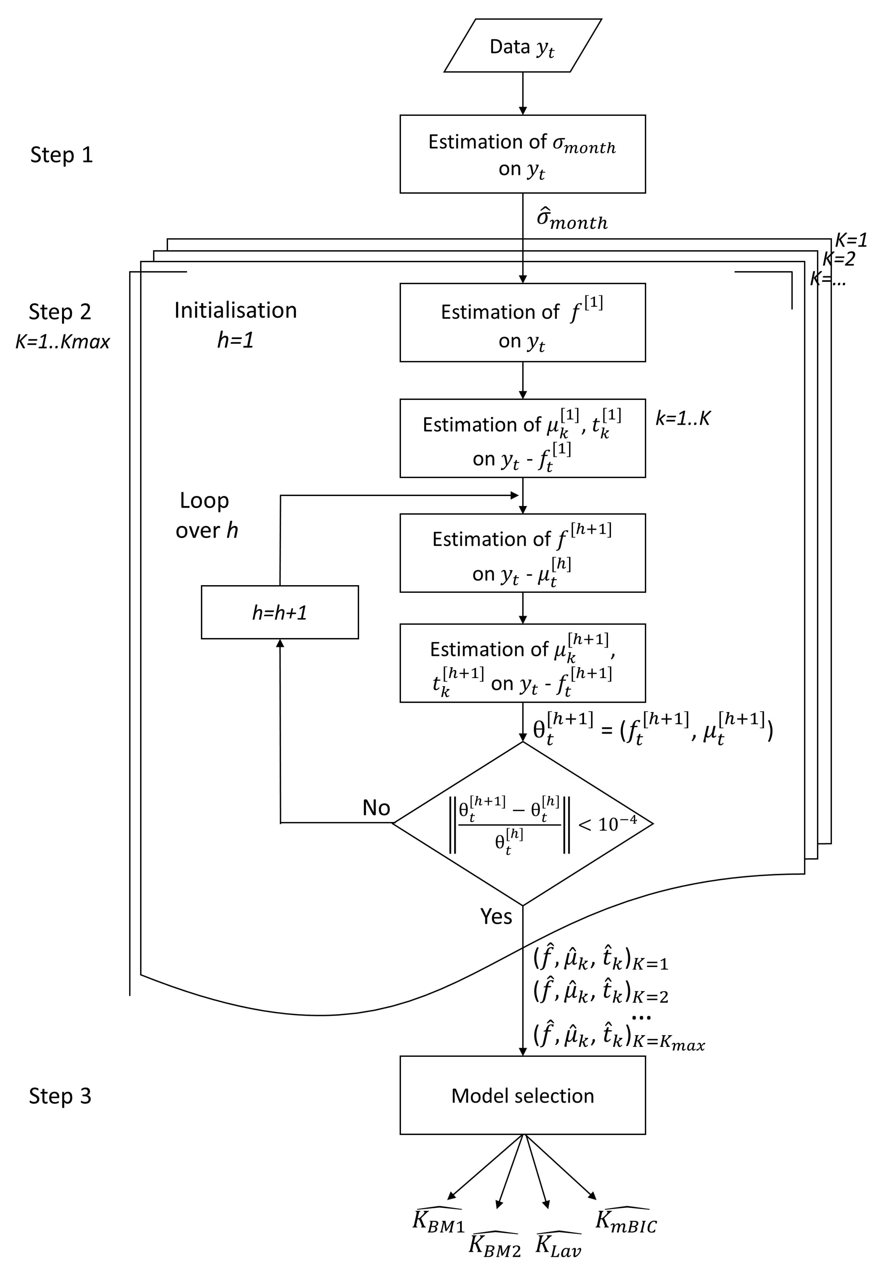
Step 1 

Estimation of ${\mathit{\sigma }}^2$. The classical sample variance estimator cannot be used here because of the presence of change points in the series. Following Bock et al. [8], we use instead the Qn estimator proposed by Rousseeuw and Croux [32], applied to the differentiated series $Y_t-Y_{t-1}$. The differentiation acts to center the series, except at the change point positions, which can be seen as outliers. Because the Qn estimator is not sensitive to outliers, the resulting variance estimator has low bias and high efficiency. The estimated variance is denoted ${\widehat{\sigma }}_{\mathrm{month}}^2$. We propose to estimate the variance parameters before we start the iterative procedure (Step 2). This choice was made after testing the alternative version in which the variance parameters are updated at each iteration of the iterative procedure. In the alternative version, the variance estimates were slightly more accurate but at the severe cost of slowing down the convergence, with no significant benefit in the segmentation results. Thus, we opted for the estimation of the variance parameters before the iterative procedure. Note that the presence of the function f in our model has little impact on the resulting variance estimation because it is a smoothly varying function (see below).

Step 2 

Estimation of f, t, and $\mathit{\mu }$. These parameters are estimated iteratively for a given K, where the variances ${\widehat{\mathit{\sigma }}}^2$ are estimated in Step 1. The estimates are obtained by maximizing the log-likelihood given by Equation (2), which is equivalent to minimizing the following squared sum of residuals, $SSR$, in a least-squares sense:

$${\mathrm{SSR}}_K(\mathit{t},\mathit{\mu },{\widehat{\mathit{\sigma }}}^2,f)=\sum _{k=1}^K\sum _{\mathrm{month}}\sum _{t\in I_k^{\mathrm{mean}}\cap I_{\mathrm{month}}^{\mathrm{var}}}\frac{{(y_t-f_t-{\mu }_k)}^2}{{\widehat{\sigma }}_{month}^2}$$

(3)

At iteration $[h+1]$:

(a)

The estimator of f results in a weighted least-squares estimator with weights $1/{\widehat{\sigma }}_{\mathrm{month}}^2$ on ${\{y_t-{\mu }_k^{\left[h\right]}\}}_t$. For our application, we follow [39] and represent f as a Fourier series of order 4, which accounts for annual, semi-annual, ter-annual, and quarter-annual periodicities in the signal:

$$f_t=\sum _{i=1}^4{a}_{i}cos\left(w_{i}t\right)+b_{i}sin\left(w_{i}t\right),$$

where $w_i=2\pi \frac{i}{L}$ is the angular frequency of period $L/i$ and L is the mean length of the year ($L=365.25$ days when time t is expressed in days). The estimated function is denoted $f^{[h+1]}$.

(b)

The segmentation parameters are estimated based on ${\{y_t-f_t^{[h+1]}\}}_t$. We obtain

$${\mu }_k^{[h+1]}=\frac{{\sum }_{\mathrm{month}}{\sum }_{t\in I_k^{\mathrm{mean}}\cap I_{\mathrm{month}}^{\mathrm{var}}}\frac{(y_t-f_t^{[h+1]})}{{\widehat{\sigma }}_{\mathrm{month}}^2}}{{\sum }_{\mathrm{month}}{\sum }_{t\in I_k^{\mathrm{mean}}\cap I_{\mathrm{month}}^{\mathrm{var}}}\frac{1}{{\widehat{\sigma }}_{\mathrm{month}}^2}},$$

and

$${\mathit{t}}^{[h+1]}=\underset{\mathit{t}\in {\mathcal{M}}_{K,n}}{argmin}\sum _{k=1}^K\sum _{\mathrm{month}}\sum _{t\in I_k^{\mathrm{mean}}\cap I_{\mathrm{month}}^{\mathrm{var}}}\frac{{(y_t-f_t^{[h+1]}-{\mu }_k^{[h+1]})}^2}{{\widehat{\sigma }}_{\mathrm{month}}^2},$$

where ${\mathcal{M}}_{K,n}=\{(t_1,\dots ,t_{K-1})\in {\mathbb{N}}^{K-1},0=t_0<t_1<\dots ,t_{K-1}<t_K=n\}$ is the set of all the possible partitions of the grid $〚1,n〛$ in K segments. This turns into a classical segmentation problem for which DP applies.

The final estimators are denoted $\widehat{f}$, $\widehat{\mathit{t}}$, and $\widehat{\mathit{\mu }}$.

Step 3 

Choice of K. This is the most delicate and difficult problem. We use three penalized least-squares-based criteria since the segmentation is conducted with ‘known’ variances. The model selection strategy consists in selecting K as follows:

$$\hat{K}=\underset{K}{argmin}{\mathrm{SSR}}_K(\widehat{\mathit{t}},\widehat{\mathit{\mu }},{\widehat{\mathit{\sigma }}}^2,\widehat{f})+pen\left(K\right)$$

where ${\mathrm{SSR}}_K$ is defined by (3). We recall the three considered criteria:

Lav 

proposed by [35] with the penalty $pen\left(K\right)=\beta K$, where $\beta$ is a penalty constant chosen using an adaptive heuristic. This heuristic involves a threshold S, which is fixed to $S=0.75$, as suggested by Lavielle [35].

BM 

proposed by [34,40] with the penalty $pen\left(K\right)=\alpha K\left(5+2log\left(\frac{n}{K}\right)\right)$, where the penalty constant $\alpha$ is calibrated using the ‘slope’ heuristics proposed by [41]. Here, we consider two heuristics, the ‘dimension jump’ and the ‘data-driven slope estimation’, which are referred to as BM1 and BM2, respectively, hereafter.

mBIC 

the modified version of the classical BIC criterion derived in the segmentation framework by [36], which is a BIC-based criterion with the integration of a penalty term depending on the segment lengths.

The estimation procedure is summarized in Figure 2.

2.3. Procedure Settings and R Packages

2.3.1. Maximal Number of Segments, $K_{\max }$

In practice, Step 2 is performed for $K=1,\dots ,K_{\max }$, where $K_{\max }$ should be 2 or 3 times larger than the expected number of change points. For both the simulations and the applications, we used $K_{\max }=30$.

2.3.2. Iterative Procedure of Step 2

Any iterative procedure needs a proper initialization procedure and a stopping rule. For the initialization, we estimate first the function f using a unweighted regression, while in the main loop, we use a weighted regression as formulated in Step 2 above. For the stopping rule, the change in $f_t$ and ${\mu }_k$ between two successive iterations is checked against a fixed threshold. The convergence of the iterative procedure is accelerated following the scheme proposed by [42]. We tested two other options: (i) estimating f using a weighted regression both in the initialization and in the main loop, and (ii) estimating first the segmentation. Both options degraded slightly the results due to the confusion between the means and the functional. For this reason, the final version of the algorithm estimates first the functional part and then the segmentation parameters.

2.3.3. Time Complexity

The segmentation (Step 2) is obtained using the DP algorithm, which reduces the algorithmic complexity from $\mathcal{O}\left(n^K\right)$, as would be the case with a naive search, to $\mathcal{O}\left(K{n}^2\right)$. The complexity of the choice of K (Step 3) is $\mathcal{O}\left(n\right)$, such that the complexity of the global method including both steps of the iterative algorithm is limited by the segmentation, i.e., $\mathcal{O}\left(K{n}^2\right)$.

2.3.4. R Packages

The method was initially implemented in an R package named GNSSseg, which is available on the CRAN. A more recent and faster version named GNSSfast is now also available from the Git repository https://github.com/arq16/GNSSfast.git (accessed on 12 June 2022). GNSSfast integrates a faster version of the DP algorithm, based on R package gfpop, proposed by Hocking et al. [43], with an algorithmic complexity in $\mathcal{O}(Knlogn)$ for the segmentation step. We evaluated empirically the time improvement of GNSSfast on an excerpt of ten series from the application data set used in Section 3 with length varying between 5000 and 6000 points. The mean time over the ten series of the procedure is 41 min (2463 s) with GNSSseg against 1.32 min (79 s) with GNSSfast on a standard PC workstation with a Ubuntu 18.04.2 LTS operating system.

2.4. Simulation Study

The performance of the new segmentation method, segfunc, was assessed by means of simulations, presented in the Supplemental Material. It is shown that the monthly variance parameters estimated in Step 1 (i.e., outside of the iterative procedure) are sufficiently accurate to allow for good performance of the subsequent segmentation. Estimating the variance terms outside of the iterative procedure also accelerates the convergence compared to the case where they are estimated inside the loop. The accuracy of the number and position of detected change points is shown to depend on the $SNR$, as expected, with some differences between the criteria. In situations of large noise, BM1, BM2, and mBIC tend to underestimate the number of change points, but with reasonable dispersion, compared to Lav, which has a smaller bias but larger dispersion. The performance of segfunc is also shown to be similar to that of segonly when no functional is simulated, and superior when a functional is simulated. As expected, in the presence of a periodic bias, segonly has a tendency to over-segment the time series in order to fit the bias with changes in the mean. This deficiency is clearly overcome with the new method.

3. Results

3.1. Data, Metadata, Outlier Detection, and Validation Procedures

The data set consists of daily IWV differences (GNSS minus ERA-Interim reanalysis), for 120 global GNSS stations, for the period from 1 January 1995 to 31 December 2010 [24,44]. A map of the station network can be found in [24]. The metadata include equipment changes and processing changes (the latter are specific to the particular reprocessed data set used in this study [45], but they concern only a few stations in 2008 and 2009; this issue is further discussed in Parracho et al. [6]). The equipment changes were extracted from the IGS site-logs (https://files.igs.org/pub/station/log/, accessed on 12 June 2022). They consist of the dates of receiver (R), antenna (A), and radome (D) changes. Experience showed that not all equipment changes produce a break in the GNSS IWV time series. The most important ones are antenna and radome changes [7]. However, there is some evidence that changes in the receiver settings can also produce inhomogeneities [5], especially changes in the elevation cutoff angle setting. Unfortunately, the elevation cutoff angle settings have not been reported in the IGS site-logs in the early periods (mainly before 2000). The GNSS IWV estimates are also impacted by environmental changes that are not reported in the IGS log-files, such as changes in the electromagnetic reflections and scattering properties of surfaces around the receiving antenna and changes in the satellite visibility (e.g., due to growing vegetation or urbanization). As a consequence, although the metadata extracted from the IGS site-logs represent a valuable source of validation, they may be incomplete and a perfect matching between our detected change points and the IGS metadata is thus not to be expected. For the validation, it is customary to use a certain time window, although there is actually no established standard for the size of this window. Values between 5 days and 183 days have been used by various authors with daily data [9,46,47]. In this study, we use a time window of ±62 days, which is consistent with the study of [9].

Another important aspect in the analysis of our segmentation results is the post-processing of clusters of change points that we are classifying as ‘outliers’. Figure 3 shows an example of a time series with three clusters detected in October 1997, in May 2004, and in May–August 2005, containing two, two, and four change points, respectively, within a time window of ±80 days. This window size was chosen after performing a mixture model analysis of the segment lengths, which showed that the distribution of segment lengths could be optimally divided into two classes with a separation length of 80 days. Moreover, we also noted that the shorter segments are associated with larger changes in means, which seem to be due to noise spikes. This can also be seen from Figure 3. We set up a screening method to reject the clusters of outliers that were not associated with a significant change in mean before and after. A weighted t-test was used for this purpose on the series corrected by the estimated periodic function. In the case of the time series shown in Figure 3, the changes in the mean before and after all three clusters are significant, meaning that they are all three associated with a change point. For these clusters, we kept the middle position of the change points as representative of the actual change point. In this specific example, the eight outliers are replaced with three significant change points, hence decreasing the total number of change points from 12 to 7.

3.2. General Results

In this section, we present global results for three versions of our segmentation method: (a) segfunc, the new method described in Section 2 of this paper (in its final form); (b) segonly, the method described in Bock et al. [8], which does not include the functional part; and (c) seghomofunc, a variant of segfunc, which considers a homoscedastic noise variance instead of a monthly one, where the single noise variance parameter is estimated during Step 2 of the method.

Figure 4 shows the distribution of the number of detected change points before screening, for the three variants of the segmentation method and the four selection criteria. The most striking feature, common to all three methods, is the significantly different results of mBIC compared to the three other criteria. This behavior was not observed with the simulations. In general, mBIC detects a number of change points close to the maximum, which is 29 (since the method is parameterized with $K_{\max }=30$). In the case of seghomofunc, the mean number of change points with mBIC is slightly decreased (19, compared to 27–28 with the other variants). This may be explained by the fact that mBIC has been derived theoretically under the assumption of homoscedasticity, independent noise, and Gaussian distribution. As shown by [48] using simulations in a Gaussian homoscedastic independent segmentation model, mBIC is much more sensitive to the distribution assumption than the other criteria. Among the other three criteria, Lav shows a broader distribution in K, which reflects the greater instability of this selection criterion (as was already seen in the simulations). This criterion selects very few cases with no change point compared to BM1 and BM2 (for segfunc, there are 6, 22, and 13 cases, for Lav, BM1, and BM2, respectively). In the case of BM1, many of these cases correspond to the situation where there are multiple maximum dimension jumps (16 out of 22, with segfunc). The mean and total numbers of change points are also larger with Lav than with the two BM criteria, with BM2 having slightly larger numbers than BM1.

Among the three variants, the mean and the total number of change points for Lav, BM1, and BM2 are larger for segfunc compared to segonly and seghomofunc. The smaller number of change points for segonly can be explained by the fact that, on average, the cost of including more change points to fit the periodic bias in the signal is too high (although this can happen in some cases, as in the introductory example of Figure 1). In the case of seghomofunc, the estimated noise variance is not representative of the actual noise, which is in general changing from one month to another. It appears that the estimated variance leads to a smaller number of change points than in the case of segfunc. Stated in another way, the segfunc method detects more change points thanks to the use of a more realistic model, i.e., this method is able to detect smaller changes in the mean. Another argument for this explanation is that the variance estimated with seghomofunc is, in general, larger than the mean variance estimated with segfunc. However, we know from the simulation study that the segmentation generally underestimates the number of change points when the noise is large, i.e., in this case, seghomofunc would underestimate the number of change points.

Table 1. Comparison of segmentation results for three variants of the method and four model selection criteria, before and after the outlier screening. The columns report the total number of detected change points, outliers, and validations with respect to the metadata (number and percentage).

	Before Screening				After Screening
	Detections	Outliers	Validations		Detections	Validations
Variant (a) segfunc
mBIC	3251	2714	415	13%	1270	263	21%
Lav	474	194	108	23%	341	102	30%
BM1	335	70	93	28%	292	93	32%
BM2	435	113	107	25%	370	105	28%
Variant (b) segonly
mBIC	3367	2123	538	16%	1865	393	21%
Lav	350	54	87	25%	316	85	27%
BM1	269	28	76	28%	253	74	29%
BM2	414	66	98	24%	378	94	25%
Variant (c) seghomofunc
mBIC	2283	1941	278	12%	678	180	27%
Lav	415	212	86	21%	249	75	30%
BM1	287	75	86	30%	242	83	34%
BM2	387	142	101	26%	295	96	33%

reports additional statistics, before and after screening, which are useful to assess the performance of the different criteria and methods. First, we note that BM1 has the smallest number of detections and outliers, and the largest percentage of validations, both before and after screening, among all four criteria. These are the most important features expected from the segmentation method and therefore make this selection criterion the preferred one, although the performance of BM2 and Lav is close, mainly after the screening. If we consider only the percentage of validation, the seghomofunc variant has slightly better performance than segfunc, but the price of this small improvement is a reduction in the total number of detections of around 20% for BM1 and BM2 and 30% for Lav after screening. Moreover, the total number of outliers with seghomofunc is larger than with segfunc by 10 to 25% for BM1, BM2, and Lav, due to the mis-modeling of the variance. In some cases, the number of detections is also larger with this variant (up to 19, compared to 13 with segfunc, as reported in Figure 4). In Section 3.3 below, we show a few examples of such cases.

Table 2. Comparison of mean and inter-quartile range (iqr) of distance of detected change points from known changes (from the metadata), for three variants and four model selection criteria. Distance unit in days.

	Before Screening		After Screening
	Median	iqr	Median	iqr
Variant (a) segfonc
mBIC	221	430	205	399
Lav	190	390	149	358
BM1	168	361	150	358
BM2	171	352	158	337
Variant (b) segonly
mBIC	219	414	224	417
Lav	183	418	175	425
BM1	163	341	157	337
BM2	193	348	188	350
Variant (c) seghomofunc
mBIC	225	423	178	376
Lav	190	370	155	340
BM1	129	320	132	336
BM2	153	354	138	333

compares the distance of detected change points from the documented changes, before and after screening. The median distance is, in all cases, smaller for BM1. The dispersion, measured by the inter-quartile range (iqr), is the smallest either for BM1 or BM2. After screening, the best performance in terms of median and iqr is found with seghomofunc, but since the number of detections is significantly smaller than with segfunc, this result may be misleading. The performance of segfunc with BM1 can be established to 150 days based on the median distance, with an iqr of 358 days. Given that the metadata may be incomplete and that the noise variance and functional in these data are relatively large (see Figure 5), this performance is satisfying. Regarding the incompleteness of the metadata, we noticed a special case (station JOZE) where no equipment was reported between August 1993 and May 2009, which seems rather suspicious (i.e., some changes may not have been reported). In this case, we found an extreme distance of 4615 days with all variants and criteria. For all other stations, the largest distance was smaller than 1500 days.

Figure 5 presents additional characteristics of the time series and detected change points in the case of segfunc and BM1. Figure 5a shows that the yearly mean standard deviation of the noise ranges between 0 and 2 kg m${}^{-2}$, with a mean value over the 120 stations of 0.84 kg m${}^{-2}$ and a range (seasonal excursion) of 0.63 kg m${}^{-2}$ on average, which reflects the importance of modeling the heterogeneous variance. Figure 5b presents a measure of the magnitude of the periodic bias with an average value of 0.33 kg m${}^{-2}$. It is clear that the periodic bias is not negligible and that it is important to model it. Figure 5c shows that the distribution of offsets (changes in mean) is nearly symmetrical, with a mean absolute value of 1.27 kg m${}^{-2}$, which is relatively large. The dip centered on zero reflects the fact that the smaller offsets are more difficult to detect because of their small signal-to-noise (SNR) ratio. The most frequently detected offsets are found around +/− 0.5 kg m${}^{-2}$. The larger offsets (up to +/− 10 kg m${}^{-2}$) are due to outliers (see, e.g., Figure 3). Figure 5d shows the distribution of SNR${}_t$, computed as the absolute value of offset divided by the standard deviation of noise. It is peaking at 0.6 and the larger values (up to 10) correspond again to outliers. The mean SNR${}_t$ of 1.55 indicates that this segmentation method has a good efficiency of detection.

3.3. Examples of Special Cases

In this section, we analyze in more detail the results for a few stations, but we consider only the results with the BM1 penalty criterion. With the segonly method, there are actually 66 stations which have the same number of detections as method segfunc. Although, in general, the change points are located at the same positions, this is not always the case. For 18 stations, variant segonly detects more change points, and for 36 stations, it detects fewer than segfunc. Station POL2 is an example of the former category and station STJO an example of the latter. DUBO is an example where the same number is detected with both variants, but the change points are not located at the same positions. With variant seghomofunc, the number of stations with equal, more, and fewer detections than segfunc is 57, 24, and 39, respectively. Examples are EBRE, MCM4, and POL2, respectively. The results for four of these stations are illustrated in Figure 6 and are discussed thereafter.

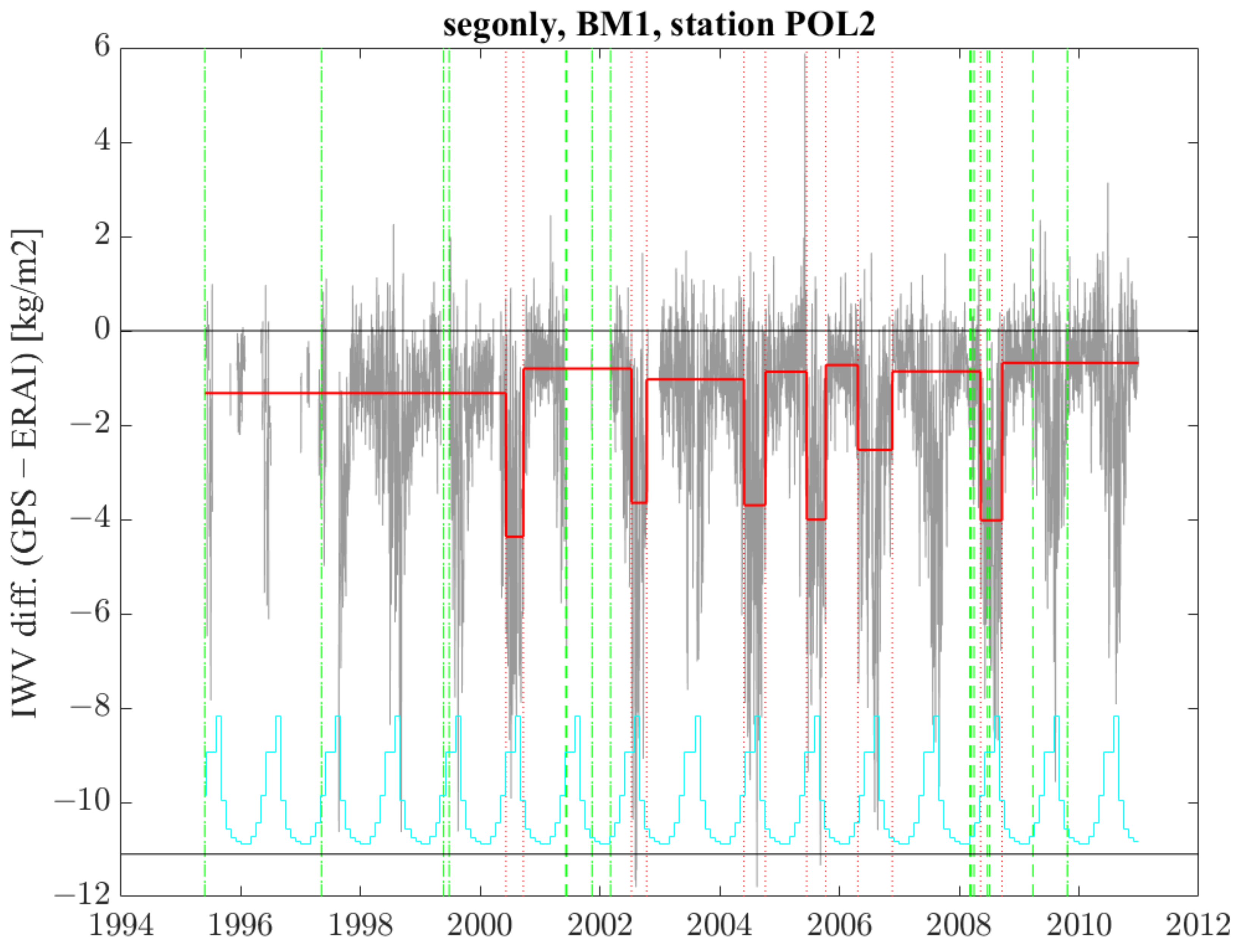
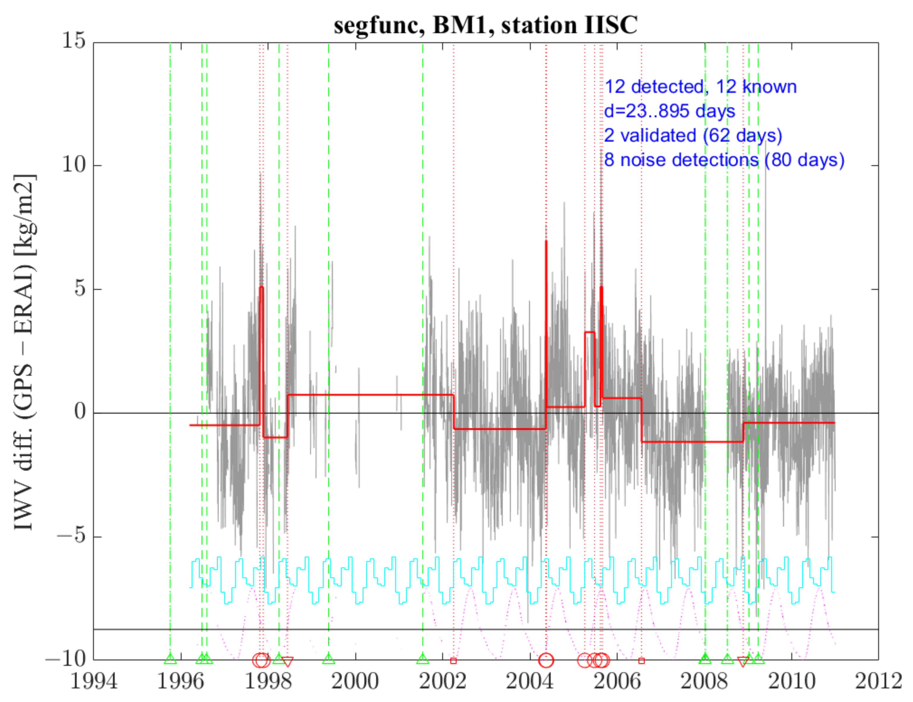
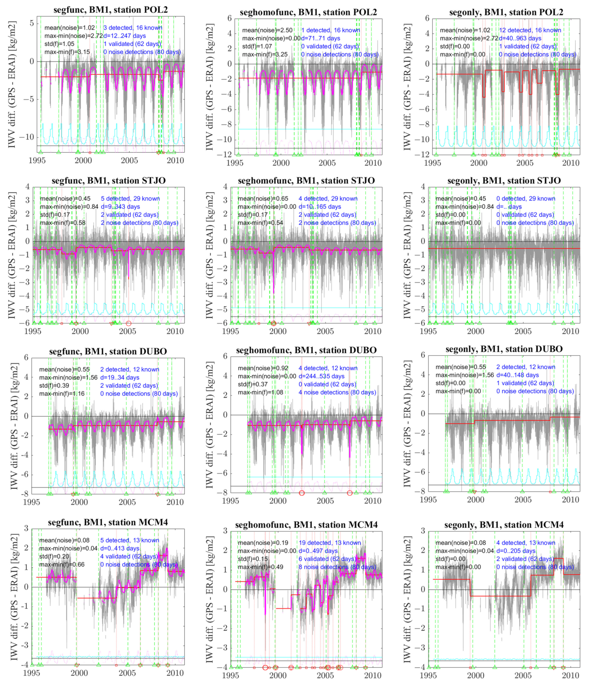
• In the case of POL2, variants segfunc, segonly, and seghomofunc detect 3, 12, and 1 change point(s), respectively. The signal shows a strong periodic variation, which is well fitted with segfunc and seghomofunc but is erroneously captured by the segmentation with segonly. Variant segfunc has one validated change point (23 February 2008), while segonly has no validation, although it detects 12 change points. Variant seghomofunc detects only one change point, which is located 72 days from the nearest known change point and is thus not validated, but it coincides with one of the three detections found by segfunc. The detection of this change point is made difficult because it is located in a month with strong noise.
• In the case of STJO, variants segfunc and seghomofunc detect five and four change points, respectively, with two similar validated change points (at 20 July 1999 and 18 April 2003) and one cluster of two outliers each. The two clusters are not at the same positions, but both are associated with a significant change in mean before/after and their outliers are thus replaced with one single change point at mid-range by the screening procedure. Variant segonly gives no detection in this case. This is due to the ‘Big Jump’ heuristic, as discussed in the section above.
• In the case of DUBO, variants segfunc and segonly detect two change points at almost the same position. Both are located close to known changes and are validated with segfunc, but only one is validated with segonly. Variant seghomofunc has two clusters of two outliers and no validation. Both clusters are associated with significant changes in mean before/after and thus two change points remain after screening. The second one is close to a change point detected by the other variants.
• Finally, for MCM4, the signal has very marked inhomogeneities in the form of several abrupt changes in the mean but also large oscillations between 2000 and 2005. The abrupt changes are well captured by segfunc, which detects five change points, among which four are validated. The non-stationary oscillations are only partly modeled by the periodic function. This is a special case where the functional model does not well capture the full signal. This result advocates for a future improvement of the modeling of the functional part. Variant segonly works quite well too and leads to almost the same detections as segfunc, but only two change points are validated. Variant seghomofunc, on the other hand, significantly overestimates the number of change points in order to fit the non-stationary oscillations. It also contains several outliers. This variant has six validated change points, with two additional ones compared to segfunc, but this may be by chance because the total number of change points is quite large.

3.4. Semi-Automatic Selection of Change Points

We have seen above that three of the penalty criteria (BM1, BM2, and Lav) used with the segfunc method behave well, in the sense that they select a reasonable number of change points and achieve a fairly good validation rate with respect to the GNSS metadata (around 30%). However, to make the final selection, it is necessary to use a decision rule, which can be either automatic or semi-automatic. We start with the semi-automatic approach, in which we use our expertise to select the ‘best’ segmentation among the solutions proposed by the three criteria. This work is done station by station, and consists of inspecting first, visually, the monthly time series with the known GNSS metadata superposed to derive a first guess of the possible change point dates. These dates are then compared to the results from the three criteria and the closest solution is accepted partly or totally. In this selection, priority is given to the change points close to known changes composed of the GNSS metadata extracted from the IGS site-log files, as well as daily quality check information produced with TEQC software (a software program widely used for the translating, editing, and quality checking of raw GNSS measurements [49]). When the choice is difficult, higher priority is also given to the solution with the smallest number of change points. For each station, the change points selected by each of the three criteria are either rejected or accepted and a corresponding flag is set. In case a change point is accepted, its date can be either set to the date of the nearest metadata, or to a better one than the nearest one (e.g., an antenna change instead of a processing change), or kept as the detected date with the flag ‘undocumented’.

Table A1. List of change points selected manually from the BM1, BM2, and Lav solutions of the segfunc method with the help of GNSS metadata (see text for details).

Name	Date	Flag	Name	Date	Flag	Name	Date	Flag
algo	12 December 2008	RC	gode	06 August 1998	U	mcm4	18 May 2006	R
algo	26 March 2009	PC	gope	26 April 1996	U	mcm4	31 March 2008	P
alic	31 July 1999	RC	gope	24 July 2000	RADGT	mcm4	26 March 2009	P
alic	20 April 2006	UC	gope	01 January 2002	UGTL	mdo1	24 December 2001	UC
ankr	24 November 2000	RAL	gope	18 January 2005	UL	mdo1	18 April 2004	UC
ankr	06 May 2008	RADGTL	guam	26 April 2000	RGT	medi	27 March 1999	UC
areq	28 January 2000	RC	guam	19 September 2004	U	medi	27 June 2004	UC
areq	23 April 2001	UC	hers	01 January 1998	RAGTC	medi	14 May 2006	UC
areq	20 August 2004	U	hers	10 September 2000	UC	monp	22 March 2000	AD
azu1	12 February 2008	RC	hob2	16 August 1999	RGTL	nlib	11 August 1998	U
azu1	03 October 2008	RC	hob2	02 April 2002	RL	nlib	12 March 2003	U
azu1	20 July 2010	R	hob2	04 October 2005	RTL	nlib	15 November 2009	U
blyt	14 May 1998	R	holb	02 January 2002	RGTC	onsa	02 February 1999	RAD
bor1	24 June 2003	UT	holb	15 November 2005	UC	penc	22 January 2001	UC
bor1	26 March 2009	P	holb	06 March 2009	RTC	penc	08 December 2003	RTC
braz	05 November 2005	T	holp	19 November 1997	R	pert	12 June 1996	R
brmu	01 October 1997	R	hrao	26 April 2000	RGTC	pert	06 June 2001	RA
brus	09 June 2006	UC	hrao	02 August 2004	UC	pert	18 August 2006	U
brus	26 October 2008	UC	hrao	23 February 2006	AGT	pin1	28 February 2001	AD
cagl	11 July 2001	RAGT	iisc	02 May 2004	UC	pots	15 January 1996	R
cas1	27 January 1996	RC	iisc	22 July 2006	UC	pots	19 August 1999	RGT
cas1	27 November 1997	UC	irkt	17 April 1998	UL	pots	15 April 2009	A
cas1	05 February 2000	RT	irkt	17 June 2003	UL	quin	13 November 2002	RA
cas1	31 March 2008	P	karr	22 August 2006	U	reyk	13 June 2003	A
cas1	02 December 2008	RPT	kely	14 September 2001	RADL	reyk	31 March 2008	P
ccjm	24 February 2001	RA	kely	11 November 2006	UL	reyk	26 March 2009	P
cedu	10 September 1997	RA	kely	17 December 2009	UL	rock	10 June 1999	RT
cfag	06 May 1997	UL	kerg	31 March 1999	RA	sant	02 November 1999	RC
cfag	21 January 2008	UL	kerg	14 November 2002	UGT	sant	14 December 2000	RC
chat	28 March 2002	RUC	kiru	01 December 2004	U	shao	08 February 2003	U
chat	31 March 2008	PC	kit3	31 March 2008	P	sio3	12 April 2000	AD
chil	30 May 1995	AD	kokb	23 July 1999	R	sni1	19 December 2000	AD
clar	12 September 1996	R	kokb	21 July 2001	U	stjo	23 January 1998	UC
coco	04 September 1998	RGT	kokb	06 December 2006	U	stjo	29 July 1999	RC
coco	09 August 2003	UL	kosg	07 December 1996	U	svtl	23 October 2008	RADT
coco	13 January 2007	UL	kosg	28 February 1999	R	syog	08 February 2000	RT
coso	09 November 2000	U	kosg	27 November 2000	!RGT	syog	25 January 2007	RGT
crfp	12 November 1997	RC	kosg	29 September 2009	U	syog	31 March 2008	P
crfp	27 May 2002	UC	kour	30 July 1999	R	syog	26 March 2009	P
crfp	07 September 2005	UC	kour	21 November 2000	U	tow2	29 August 1998	U
cro1	30 September 1999	R	kour	30 September 2004	R	tow2	01 November 2003	U
cro1	04 August 2005	RAD	kour	13 December 2009	U	tow2	14 February 2006	RT
darw	21 June 1998	UT	lama	06 October 2000	AD	trak	04 August 1995	AD
darw	23 December 2003	UC	lbch	01 September 1998	U	trak	05 February 2004	U
darw	03 November 2005	UC	lbch	05 February 2004	U	uclu	16 May 2003	UC
dav1	14 March 2002	UC	long	04 April 1995	RA	uclu	04 May 2007	RACT
dav1	27 January 2003	UC	long	05 September 1996	R	usud	05 October 2000	RT
dav1	31 March 2008	P	long	25 March 2001	U	vill	18 July 2000	R
dav1	31 January 2009	P	long	02 January 2007	U	vill	03 December 2004	R
dav1	04 May 2010	R	lpgs	02 May 2003	U	vndp	17 March 1996	R
dgar	15 November 2006	U	lpgs	30 August 2006	?	wes2	05 February 1998	R
dhlg	23 December 1999	R	mac1	04 January 2001	R	wes2	26 July 2000	RA
drao	08 October 1999	RGT	madr	18 August 1999	R	wes2	29 June 2001	RA
dubo	04 October 1999	RAD	madr	07 November 2004	U	wlsn	18 August 1997	U
dubo	31 March 2008	P	mas1	14 August 1999	R	wlsn	11 January 2000	U
ebre	23 February 1999	U	mas1	30 March 2006	U	wlsn	29 March 2006	U
ebre	16 November 2005	RT	mate	25 September 2001	R	wslr	29 March 2000	RAD
fair	03 June 1999	RTC	maw1	07 November 1997	U	wtzr	30 June 2009	R
fair	15 April 2000	RTC	maw1	22 August 1999	R	wuhn	08 June 2000	RAD
fale	04 September 1998	UC	maw1	07 December 2004	RT	wuhn	18 September 2006	U
fale	01 June 2001	UC	maw1	04 May 2010	R	yell	22 August 1996	A
flin	21 September 1999	AD	mcm4	07 September 1999	R
flin	03 January 2008	P	mcm4	13 November 2003	UGT

lists the final results for all stations with accepted change points (91 out of 120 stations, i.e., based on our manual selection, 29 stations have no change point).

Table 3. The number of change points before and after screening from method segfunc, and the number of change points accepted by manual decision and validated by GNSS metadata (either with IGS metadata only or with IGS metadata plus TEQC results, last column). The percentage of accepted and validated change points is computed with respect to the number after screening and accepted, respectively.

	Before	After	Accepted	Validated (Metadata)	Validated (+TEQC)
BM1	335	292	168 (57%)	99 (58.9%)	105 (62.5%)
BM2	435	370	166 (45%)	99 (59.6%)	105 (63.3%)
Lav	474	341	175 (51%)	103 (58.9%)	109 (62.3%)
total			187	110 (58.8%)	116 (62.0%)

summarizes the results from the manual validation. It can be seen that a larger number of change points have been accepted with the Lav criterion (175 out of 187), although the percentage of accepted change points is slightly larger for BM1, while both the number and percentage are smaller for BM2. Based on this result, BM1 and Lav appear to be more adapted. The numbers of validations with respect to the IGS metadata and TEQC results are quite similar among the criteria, demonstrating that the selection process was performed consistently among the three criteria. It is also noteworthy that the validation rate of the accepted change points significantly increases compared to the results before and after the screening. The validation percentage reaches almost 59% based on IGS metadata only and 62% when TEQC results are included.

The results from this semi-automatic approach were analyzed in order to check if simple rules can be derived that could be used in a fully automatic selection procedure. Therefore, we address the following questions:

(1)

Is there any one criterion that performs well and could be used systematically?

(2)

Is the solution with the smallest number of change points a better choice?

(3)

Is the solution selected by more than one criterion a better choice?

Question 1 was already partly answered above, with BM1 showing a higher percentage of acceptance. In addition, we also checked how many times each of the criteria was accepted totally (i.e., all the change points were accepted). Again, BM1 achieved the highest score, with 62%, followed by Lav with 58% and BM2 with 42%. Not only BM1 does perform better, but its success rate reaches 90% (168 change points accepted out of 187). Thus, we conclude that if one wishes to chose one specific criterion, it should be BM1. Regarding question 2, we found that with BM1, the solution with the smallest number of change points is adopted in 60% of the cases, compared to 57% for Lav, and 38% for BM2. These results reflect the fact that there are a number of cases where only a few or none of the detected change points are accepted. Regarding question 3, the fraction of cases when two or three criteria are consistent, after the screening, ranges between 52% (BM1 and BM2 consistent) and 63% (BM1 and Lav consistent). The special case when all three criteria are consistent and accepted amounts to 58%. Thus, consistency between the three criteria is not a sufficient condition for accepting all the detected change points. It thus emerges that neither the solution with the smallest number of change points, nor the one when all three criteria are consistent, is a sufficiently good option for a fully automatic selection. Moreover, choosing the best criterion, BM1, also only achieves a validation rate of 62%. We recommend thus to use the semi-automatic validation method based on the station-by-station inspection of the results from the three criteria, as described above.

4. Discussion and Conclusions

This paper described an extension of the segmentation method developed by [8] (segonly), which is dedicated to detecting abrupt changes in the mean in the presence of a variance changing on known, fixed, intervals. The new method, called segfunc, includes a function f representing a time-varying bias in the data (in the first instance, a periodic bias is modeled). It implements an iterative procedure to estimate sequentially the function by a weighted least-squares regression and the segmentation parameters (position and amplitude of change points) by means of a Dynamic Programming algorithm. Both methods have been tested and compared in a simulation framework (see the Supplemental Material). They performed similarly when no periodic bias was simulated. However, in the presence of a periodic bias, segonly had a tendency to over-segment the time series, in order to fit the bias with changes in the mean. A third version of the method, called seghomofunc, which implements the bias function but assumes a homogeneous variance, was also tested with the real data.

All the methods have been applied to real data from a network of 120 global GNSS stations with observations spanning a 16-year period. The GNSS IWV data were beforehand differenced with respect to ERA-Interim reanalysis data to remove the climatic signal. As the correction is not perfect, a residual periodic bias and a monthly varying variance can be present in the IWV differences. It is important that these characteristics are well taken into account in the segmentation method. Note that some preliminary work with the more recent ECMWF reanalysis, ERA5 Hersbach et al. [50], showed similar bias and variance features and the segmentation results with ERA5 were not quite different. The GNSS station history is well documented and was used for the validation of the detected change points. All three methods achieved very similar hit rates, around $32\%$ after screening. However, segonly and seghomofunc deviated strongly from segfunc in the presence of a significant periodic bias. In a few cases, it was observed that the segmentation captures the periodic bias, leading these methods to detect many false change points. However, in general, both methods rather underestimate the number of change points (often selecting no change point at all) because the cost of adjusting the signal would require too many change points. These results demonstrate the superior performance of the proposed segfunc method.

One critical feature in penalized maximum likelihood methods is the choice of the penalty criterion. In this work, we used two versions of the criterion proposed by Birgé and Massart [40], the modified BIC (mBIC) derived by Zhang and Siegmund [36], and the criterion proposed by Lavielle [35]. From the simulation study, Lavielle’s criterion appeared more unstable, with large dispersion in the number of detected change points, compared to the other criteria, which were more conservative, with an underestimation of the number of change points in the presence of large noise. These features were also observed with the real data, with a tendency of all criteria to detect change points preferably in the months with smaller variance. A notable difference between the simulations and real data was found with mBIC, which strongly over-segmented the real data. It is known that mBIC is more sensitive than the other criteria to the Gaussian distribution assumption [48]. Other criteria, such as, e.g., the Minimum Description Length (MDL) [51], were used by some authors in the specific climate context [19,31]. According to Ardia et al. [52], the MDL criterion can be seen as a Bayesian criterion with an appropriate prior distribution for change point models. The obtained MDL-based penalties have thus essentially the same properties as the mBIC and were not considered in our framework.

Another specific feature found with all the methods tested is the occurrence of clusters of change points. We attributed this feature to noise spikes (outlying observations) and applied a post-processing step to the estimated change points to screen out those change points that did not show a significant change in the means before and after the clusters. This behavior was also reported by [47] with the MDL penalty applied to daily temperature data. Another option to reduce the influence of these outliers would be to apply a stronger screening on the IWV differences, before running the segmentation, but with the drawback of introducing more gaps in the time series. This option was thus not considered here.

The final selection was made by a semi-automatic validation procedure in which the change points detected by the three penalty criteria that performed best (BM1, BM2, and Lavielle) with the segfunc method were checked manually. More than 50% of the detected change points were accepted, among which more than 60% could be explained by the metadata. In the end, a total of 187 change points were selected for the 120 stations of the IGS repro1 GNSS data set, which corresponds to a mean number of change points per station of 1.62 over a 16-year period, i.e., approximately one change point every 10 years. The final list of change points is provided in Appendix A. The next step in the homogenization procedure will be the correction of the GNSS series for the selected change points following, e.g., the methodology of [9].

Future improvements of the proposed segmentation method would be: (i) to consider other models for the function f since it was found that, in some cases, such as at station MCM4, a simple periodic function may be insufficient; and (ii) to take the time dependence (autocorrelation) in the data into account. The first point can be handled by an estimation of the function f using a non-parametric approach. The second point can be developed by following the approach of Chakar et al. [53], who proposed to model the temporal correlation using an autoregressive process of order 1 in a mean segmentation Gaussian process. These authors also proposed a two-stage whitening inference strategy that allows the use of the DP algorithm and find the exact maximum likelihood solution.

References

- Trenberth, K.E.; Jones, P.D.; Ambenje, P.; Bojariu, R.; Easterling, D.; Klein Tank, A.; Parker, D.; Rahimzadeh, F.; Renwick, J.A.; Rusticucci, M.; et al. Observations. Surface and Atmospheric Climate Change. In IPCC Fourth Assessment Report: Climate Change 2007; Working Group I: The Physical Science Basis; Cambridge University Press: Cambridge, UK, 2007; Chapter 3; pp. 235–336. [Google Scholar]
- Held, I.M.; Soden, B.J. Water vapor feedback and global warming. Annu. Rev. Energy Environ. 2000, 25, 445–475. [Google Scholar] [CrossRef] [Green Version]
- Nilsson, T.; Elgered, G. Long-term trends in the atmospheric water vapor content estimated from ground-based GPS data. J. Geophys. Res. Atmos. 2008, 113. [Google Scholar] [CrossRef] [Green Version]
- Bock, O.; Willis, P.; Lacarra, M.; Bosser, P. An inter-comparison of zenith tropospheric delays derived from DORIS and GPS data. Adv. Space Res. 2010, 46, 1408–1447. [Google Scholar] [CrossRef]
- Vey, S.; Dietrich, R.; Fritsche, M.; Rülke, A.; Steigenberger, P.; Rothacher, M. On the homogeneity and interpretation of precipitable water time series derived from global GPS observations. J. Geophys. Res. Atmos. 2009, 114. [Google Scholar] [CrossRef] [Green Version]
- Parracho, A.C.; Bock, O.; Bastin, S. Global IWV trends and variability in atmospheric reanalyses and GPS observations. Atmos. Chem. Phys. 2018, 18, 16213–16237. [Google Scholar] [CrossRef] [Green Version]
- Ning, T.; Wickert, J.; Deng, Z.; Heise, S.; Dick, G.; Vey, S.; Schöne, T. Homogenized Time Series of the Atmospheric Water Vapor Content Obtained from the GNSS Reprocessed Data. J. Clim. 2016, 29, 2443–2456. [Google Scholar] [CrossRef]
- Bock, O.; Collilieux, X.; Guillamon, F.; Lebarbier, E.; Pascal, C. A breakpoint detection in the mean model with heterogeneous variance on fixed time intervals. Stat. Comput. 2020, 30, 195–207. [Google Scholar] [CrossRef] [Green Version]
- Van Malderen, R.; Pottiaux, E.; Klos, A.; Domonkos, P.; Elias, M.; Ning, T.; Bock, O.; Guijarro, J.; Alshawaf, F.; Hoseini, M.; et al. Homogenizing GPS Integrated Water Vapor Time Series: Benchmarking Break Detection Methods on Synthetic Data Sets. Earth Space Sci. 2020, 7, e2020EA001121. [Google Scholar] [CrossRef] [Green Version]
- Jones, P.D.; Raper, S.C.B.; Bradley, R.S.; Diaz, H.F.; Kellyo, P.M.; Wigley, T.M.L. Northern Hemisphere Surface Air Temperature Variations: 1851–1984. J. Clim. Appl. Meteorol. 1986, 25, 161–179. [Google Scholar] [CrossRef] [Green Version]
- Easterling, D.; Peterson, T. A new method for detecting undocumented discontinuities in climatological time series. Int. J. Climatol. 1995, 15, 369–377. [Google Scholar] [CrossRef]
- Peterson, T.C.; Easterling, D.R.; Karl, T.R.; Groisman, P.; Nicholls, N.; Plummer, N.; Torok, S.; Auer, I.; Boehm, R.; Gullett, D.; et al. Homogeneity adjustments of in situ atmospheric climate data: A review. Int. J. Climatol. J. R. Meteorol. Soc. 1998, 18, 1493–1517. [Google Scholar] [CrossRef]
- Caussinus, H.; Mestre, O. Detection and correction of artificial shifts in climate series. J. R. Stat. Soc. Ser. Appl. Stat. 2004, 53, 405–425. [Google Scholar] [CrossRef]
- Menne, M.J.; Williams, C.N. Detection of Undocumented Changepoints Using Multiple Test Statistics and Composite Reference Series. J. Clim. 2005, 18, 4271–4286. [Google Scholar] [CrossRef]
- Szentimrey, T. Development of MASH homogenization procedure for daily data. In Proceedings of the Fifth Seminar for Homogenization and Quality Control in Climatological Databases, Budapest, Hungary, 29 May–2 June 2006; WMO/TD- No. 1493, WCDMP- No. 71. pp. 123–130. [Google Scholar]
- Reeves, J.; Chen, J.; Wang, X.L.; Lund, R.; Lu, Q.Q. A Review and Comparison of Changepoint Detection Techniques for Climate Data. J. Appl. Meteorol. Climatol. 2007, 46, 900–915. [Google Scholar] [CrossRef]
- Costa, A.C.; Soares, A. Homogenization of Climate Data: Review and New Perspectives Using Geostatistics. Math. Geosci. 2009, 41, 291–305. [Google Scholar] [CrossRef]
- Venema, V.K.C.; Mestre, O.; Aguilar, E.; Auer, I.; Guijarro, J.A.; Domonkos, P.; Vertacnik, G.; Szentimrey, T.; Stepanek, P.; Zahradnicek, P.; et al. Benchmarking homogenization algorithms for monthly data. Clim. Past 2012, 8, 89–115. [Google Scholar] [CrossRef] [Green Version]
- Lu, Q.; Lund, R.; Lee, T.C.M. An MDL approach to the climate segmentation problem. Ann. Appl. Stat. 2010, 4, 299–319. [Google Scholar] [CrossRef] [Green Version]
- Lund, R.; Wang, X.L.; Lu, Q.Q.; Reeves, J.; Gallagher, C.; Feng, Y. Changepoint Detection in Periodic and Autocorrelated Time Series. J. Clim. 2007, 20, 5178–5190. [Google Scholar] [CrossRef] [Green Version]
- Jones, J.; Guerova, G.; Douša, J.; Dick, G.; de Haan, S.; Pottiaux, E.; Bock, O.; Pacione, R.; van Malderen, R. Advanced GNSS Tropospheric Products for Monitoring Severe Weather Events and Climate: COST Action ES1206 Final Action Dissemination Report; Springer International Publishing: Cham, Switzerland, 2020. [Google Scholar] [CrossRef]
- Arlot, S.; Celisse, A. Segmentation of the mean of heteroscedastic data via cross-validation. Stat. Comput. 2010, 21, 613–632. [Google Scholar] [CrossRef] [Green Version]
- Dee, D.P.; Uppala, S.; Simmons, A.; Berrisford, P.; Poli, P.; Kobayashi, S.; Andrae, U.; Balmaseda, M.; Balsamo, G.; Bauer, D.P.; et al. The ERA-Interim reanalysis: Configuration and performance of the data assimilation system. Q. J. R. Meteorol. Soc. 2011, 137, 553–597. [Google Scholar] [CrossRef]
- Bock, O.; Parracho, A. Consistency and representativeness of integrated water vapour from ground-based GPS observations and ERA-Interim reanalysis. Atmos. Chem. Phys. 2019, 19, 9453–9468. [Google Scholar] [CrossRef] [Green Version]
- Auger, I.E.; Lawrence, C.E. Algorithms for the optimal identification of segment neighborhoods. Bull. Math. Biol. 1989, 51, 39–54. [Google Scholar] [CrossRef]
- Killick, R.; Fearnhead, P.; Eckley, I.A. Optimal Detection of Changepoints with a Linear Computational Cost. J. Am. Stat. Assoc. 2012, 107, 1590–1598. [Google Scholar] [CrossRef]
- Rigaill, G. A pruned dynamic programming algorithm to recover the best segmentations with 1 to Kmax change-points. J. Société Française Stat. 2015, 156, 180–205. [Google Scholar]
- Maidstone, R.; Hocking, T.; Rigaill, G.; Fearnhead, P. On Optimal Multiple Changepoint Algorithms for Large Data. Stat. Comput. 2017, 27, 519–533. [Google Scholar] [CrossRef] [Green Version]
- Bai, J.; Perron, P. Computation and analysis of multiple structural change models. J. Appl. Econom. 2003, 18, 1–22. [Google Scholar] [CrossRef] [Green Version]
- Picard, F.; Robin, S.; Lavielle, M.; Vaisse, C.; Daudin, J.J. A statistical approach for array CGH data analysis. BMC Bioinform. 2005, 6, 27. [Google Scholar] [CrossRef] [Green Version]
- Li, S.; Lund, R. Multiple Changepoint Detection via Genetic Algorithms. J. Clim. 2012, 25, 674–686. [Google Scholar] [CrossRef]
- Rousseeuw, P.J.; Croux, C. Alternatives to the Median Absolute Deviation. J. Am. Stat. Assoc. 1993, 88, 1273–1283. [Google Scholar] [CrossRef]
- Bertin, K.; Collilieux, X.; Lebarbier, E.; Meza, C. Semi-parametric segmentation of multiple series using a DP-Lasso strategy. J. Stat. Comput. Simul. 2017, 87, 1255–1268. [Google Scholar] [CrossRef]
- Lebarbier, E. Detecting Multiple Change-Points in the Mean of Gaussian Process by Model Selection. Signal Process. 2005, 85, 717–736. [Google Scholar] [CrossRef] [Green Version]
- Lavielle, M. Using penalized contrasts for the change-point problem. Signal Process. 2005, 85, 1501–1510. [Google Scholar] [CrossRef] [Green Version]
- Zhang, N.R.; Siegmund, D.O. A Modified Bayes Information Criterion with Applications to the Analysis of Comparative Genomic Hybridization Data. Biometrics 2007, 63, 22–32. [Google Scholar] [CrossRef] [PubMed]
- Truong, C.; Oudre, L.; Vayatis, N. Selective review of offline change point detection methods. Signal Process. 2020, 167, 107299. [Google Scholar] [CrossRef] [Green Version]
- Gazeaux, J.; Lebarbier, E.; Collilieux, X.; Métivier, L. Joint segmentation of multiple GPS coordinate series. J. Société Française Stat. 2015, 156, 163–179. [Google Scholar]
- Weatherhead, E.C.; Reinsel, G.C.; Tiao, G.C.; Meng, X.; Choi, D.; Cheang, W.; Keller, T.; DeLuisi, J.; Wuebbles, D.J.; Kerr, J.B.; et al. Factors affecting the detection of trends: Statistical considerations and applications to environmental data. JGR Atmos. 1998, 103, 17149–17161. [Google Scholar] [CrossRef]
- Birgé, L.; Massart, P. Gaussian model selection. J. Eur. Math. Soc. 2001, 3, 203–268. [Google Scholar] [CrossRef] [Green Version]
- Arlot, S.; Massart, P. Data-driven calibration of penalties for least-squares regression. J. Mach. Learn. Res. 2009, 10, 245–279. [Google Scholar]
- Varadhan, R.; Roland, C. Simple and globally convergent methods for accelerating the convergence of any EM algorithm. Scand. J. Stat. 2008, 35, 335–353. [Google Scholar] [CrossRef]
- Hocking, T.D.; Rigaill, G.; Fearnhead, P.; Bourque, G. Generalized Functional Pruning Optimal Partitioning (GFPOP) for Constrained Changepoint Detection in Genomic Data. arXiv 2018, arXiv:1810.00117. [Google Scholar] [CrossRef]
- Bock, O. GPS Data: Daily and Monthly Reprocessed IWV Data from 120 Global GPS Stations, Version 1.2. 2016. Available online: https://observations.ipsl.fr/espri/metadata/global_gps_iwv_v1.2.html (accessed on 12 June 2022).
- Byun, S.H.; Bar-Sever, Y.E. A new type of troposphere zenith path delay product of the international GNSS service. J. Geod. 2009, 83, 1–7. [Google Scholar] [CrossRef] [Green Version]
- Gazeaux, J.; Williams, S.; King, M.; Bos, M.; Dach, R.; Deo, M.; Moore, A.W.; Ostini, L.; Petrie, E.; Roggero, M.; et al. Detecting offsets in GPS time series: First results from the detection of offsets in GPS experiment. J. Geophys. Res. Solid Earth 2013, 118, 2397–2407. [Google Scholar] [CrossRef] [Green Version]
- Hewaarachchi, A.P.; Li, Y.; Lund, R.; Rennie, J. Homogenization of Daily Temperature Data. J. Clim. 2017, 30, 985–999. [Google Scholar] [CrossRef]
- Lebarbier, É. Discussion on “Minimal penalties and the slope heuristic: A survey” by Sylvain Arlot. J. Société Française Stat. 2019, 160, 140–149. [Google Scholar]
- Estey, L.; Meertens, C. TEQC: The Multi-Purpose Toolkit for GPS/GLONASS Data. GPS Solut. 1999, 3, 42–49. [Google Scholar] [CrossRef]
- Hersbach, H.; Bell, B.; Berrisford, P.; Hirahara, S.; Horányi, A.; Muñoz-Sabater, J.; Nicolas, J.; Peubey, C.; Radu, R.; Schepers, D.; et al. The ERA5 Global Reanalysis. Q. J. R. Meteorol. Soc. 2020, 146, 1999–2049. [Google Scholar] [CrossRef]
- Rissanen, J. Modeling by shortest data description. Automatica 1978, 14, 465–471. [Google Scholar] [CrossRef]
- Ardia, D.; Dufays, A.; Criado, C.O. Frequentist and Bayesian Change-Point Models: A Missing Link. SSRN Electron. J. 2019. [Google Scholar] [CrossRef]
- Chakar, S.; Lebarbier, E.; Lévy-Leduc, C.; Robin, S. A robust approach for estimating change-points in the mean of an AR(1) process. Bernoulli 2017, 23, 1408–1447. [Google Scholar] [CrossRef]