Verification and Validation of the COSMIC-2 Excess Phase and Bending Angle Algorithms for Data Quality Assurance at STAR

Abstract

In recent years, Global Navigation Satellite System (GNSS) radio occultation (RO) has become a critical observation system for global operational numerical weather prediction. Constellation Observing System for Meteorology, Ionosphere, Climate (COSMIC) 2 (COSMIC-2) has been a backbone RO mission for NOAA. NOAA also began to purchase RO data from commercial sources in 2020. To ensure the consistent quality of RO data from different sources, NOAA Center for Satellite Applications and Research (STAR) has developed capabilities to process all available RO data from different missions. This paper describes the STAR RO processing systems which convert the pseudo-range and carrier phase observations to excess phases and bending angles (BAs). We compared our COSMIC-2 data products with those processed by the University Corporation for Atmospheric Research (UCAR) COSMIC Data Analysis and Archive Center (CDAAC). We processed more than twelve thousand COSMIC-2 occultation profiles. Our results show that the excess phase difference between UCAR and STAR is within a few centimeters at high altitudes, although the difference increases towards the lower atmosphere. The BA profiles derived from the excess phase are consistent with UCAR. The mean relative BA differences at impact height from 10 to 30 km are less than 0.1% for GLObal NAvigation Satellite System (GLONASS) L2C signals and Global Positioning System (GPS) L2C and L2P signals. The standard deviations are 1.15%, 1.15%, and 1.32% for GLONASS L2C signal and for GPS L2C and L2P signals, respectively. The BA profiles agree with those derived from European Center for Medium-range Weather Forecast (ECMWF) reanalysis version 5 (ERA5). The Signal-to-Noise-Ratio (SNR) plays an essential role in the processing. The STAR BA profiles with higher L1 SNRs (L1 at 80 km) tend to yield more consistent results than those from UCAR, with a negligible difference and a smaller deviation than lower SNR profiles. Profiles with lower SNR values tend to show a more significant standard deviation towards the surface during the open-loop stage in the lower troposphere than those of higher SNR. We also found that the different COSMIC-2 clock solutions could contribute to the significant relative BA difference at high altitudes; however, it has little effect on the lower troposphere comparisons given larger BA values.

1. Introduction

The Constellation Observing System for Meteorology, Ionosphere, Climate (COSMIC) 2 mission and Formosa Satellite Mission 7 (COSMIC-2/FORMOSAT−7, hereafter COSMIC-2) is the backbone Global Navigation Satellite System (GNSS) Radio Occultation (RO) mission in National Oceanic and Atmospheric Administration (NOAA). Launched on June 25, 2019, the COSMIC-2 is a six-satellite constellation at 720 km altitude. Each COSMIC-2 satellite is equipped with a Tri-band GNSS (TriG) Receiver System (TGRS), which can receive RO signals emitted from GPS (Global Positioning System), GLONASS (GLObal NAvigation Satellite System), and GALILEO systems. The COSMIC-2 TGRS’s high gain antennas have a superior signal-to-noise ratio (SNR) to previous RO missions [1]. The early analysis demonstrated that COSMIC-2 data have a deeper penetration depth in the lower troposphere than other RO missions [1,2].

Numerical studies have demonstrated that the neutral atmospheric parameters derived from active GNSS RO technology are crucial for atmospheric applications [1,3,4,5,6,7,8,9,10,11,12,13,14,15,16,17,18,19]. However, the RO observation errors in the moisture lower troposphere are significant [1], and residual ionospheric errors are usually not completely removed with the first-order approximation [20]. A previous study indicated that the impacts of RO observations on numerical weather prediction (NWP) are mainly from 10 to 25 km altitudes and decrease sharply to atmospheres above and below, respectively [21]. COSMIC-2 bending angle assimilation into operational NWPs also showed positive impacts on the similar height as other RO missions [22].

With the precise positions and velocity of the Low Earth Orbit (LEO) and GNSS satellites, the time and path delay signal caused by the atmospheric refraction can be converted to atmospheric parameters, including bending angle, refractivity, temperature, moisture, and pressure in the neutral atmosphere [23]. To derive bending angle and refractivity profile from raw occultation measurements, we need to perform complicated L0-L1 (from raw data to excess phase) and L1-L2 (converting excess phase to bending angle) processing. The inversion procedures (see Figure 1) include: (i) precise orbit determination (POD) for the LEO satellite, (ii) occultation excess phase calculation with the clock bias removal and geometric range removal, and the accurate estimate of antenna phase center position in Earth-Centered Inertial (ECI) Coordinate System, (iii) inversion of bending angle from excess phase, (iv) conversion of bending angle to refractivity and other high-level products, and (v) quality control of the data products. A previous study showed that the uncertainty from excess phase conversion might propagate to bending angle retrievals [24]. The uncertainty in each step requires a detailed analysis of the error propagation and impacts on the next step.

The COSMIC-2 implementation-related uncertainties may primarily arise from the following three factors:

(i)

POD calculation for the LEO satellite

The POD process determines the LEO satellites’ mass center and the estimation of the receiver clock bias and dynamically interpolates the GNSS satellite position. The mass center position determines the antenna position and the geometric distance between receiver and transmitter to derive the geometric free excess phase later. The receiver clock bias from the POD process is used to correct the time tag in the excess phase calculation [25]. The POD (orbital) errors may introduce velocity errors, affecting the accuracy of excess phase calculation (see Section 3). Note that the orbital estimates can differ from processing software and configurations. Previous studies showed that the COSMIC-1 orbital difference could have a 10 cm mean root mean square (RMS) difference among different processing centers [26]. With different dynamic models, clock bias removal methods, and the arc-integration lengths of the POD processing, the orbital solution can vary from a few centimeters (cm) to more than 10 cm, which will lead to extra bending angle estimate uncertainty. The operational COSMIC-2 POD calculation is based on the short-arc (around one hour) solution. Because of the different clock systems and the signal frequencies among GPS, GLONASS, and GALILEO, the quality of COSMIC-2 LEO POD solutions may also be different [27]. The POD for the COSMIC-2 mission post-processing requirement is within 10 cm for position and 0.1 mm/s for velocity.

(ii)

Conversion of the COSMIC-2 carrier phase to excess phases

The different procedures for clock bias removal, the direct geometric range removal, and the antenna phase center position in the ECI Coordinate System may also introduce uncertainty in the excess phase calculations (see [25,28]). The different phase models may also lead to excess phase calculation errors. For example, the open-loop phase model for the excess phase cycle slip removal for receivers with open-loop tracking may lead to extra bending angle uncertainties in the lower troposphere [29]. Schreiner et al. [25] showed that the single and double-difference clock removal methods for COSMIC-1 with different sampling intervals in excess phase could yield about 1% fractional refractivity difference at high altitudes. Due to different transmitter/receiver clock removal methods and the open-loop phase model, we must carefully quantify the COSMIC-2 bending angle and refractivity retrieval uncertainties.

(iii)

Inversion of excess phase to bending angle

Different implementations of excess phase to the bending angle can also introduce bending angle retrieval uncertainty. Steiner et al. [30] compared the reprocessed RO products of different missions, including Meteorological Operational satellite (Metop) GNSS Receiver for Atmospheric Sounder (GRAS), Challenging Minisatellite Payload (CHAMP), Gravity Recovery and Climate Experiment (GRACE), and COSMIC-1, with different processing centers. The results showed that the mean inter-center bending angle fractional differences were minimal between 10 and 30 km impact height, less than 0.1% for all missions, and can be more than 1% above 50 km for CHAMP. Xu and Zou [31] compared the Metop-A/B GRAS data reprocessed by UCAR and Radio Occultation Meteorology Satellite Application Facilities (ROM SAF) and found that ROM SAF processed bending angle has a negative difference (ROM SAF minus UCAR) even after strict quality control, especially near the surface over the tropical area. Gorbunov et al. [32] compared their bending angle results with UCAR (using the same excess phase). The bending angle is consistent with a 0.1% mean difference above impact height of 5 km from different bending angle algorithms. These inter-center comparison results are critical for understanding the error magnitude for other reprocessing procedures and how the uncertainty propagates to the downstream products. For COSMIC-2, Adhikari et al. [33] converted the UCAR operational excess phase to bending angle using the full spectrum inversion method. The study showed that the bending angle profiles agree well with UCAR and the European Center for Medium-range Weather Forecast (ECMWF) reanalysis version 5 (ERA5) with less than the 0.1% mean difference between 8 and 40 km altitude and a standard deviation (STD) range of 1.4–2.3%.

The current near-real-time COSMIC-2 products are processed by UCAR COSMIC Data Analysis and Archive Center (CDAAC) [34]. The quality of the UCAR processed COSMIC-2 data has been assessed in terms of precision, stability, and accuracy [1]. The STAR’s L1a-L1b processing is also briefly outlined [35]. However, how the L1a-L1b processing, including implementing LEO satellite POD calculation and converting the COSMIC-2 carrier phase to excess phases, will affect the COSMIC-2 bending angel profiles was not explicitly quantified.

This study aims to quantify the uncertainty of COSMIC-2 bending angle profiles caused by the excess phase processing and bending angle inversion approaches. Studies (i.e., [3,6,30,36]) demonstrated that the best way to quantify the retrievals uncertainty from RO data products is to compare them to those derived from the independently processed data products. To understand the COSMIC-2 data uncertainty induced in each step of the RO processing, the NOAA NESDIS/STAR developed an independent processing package (hereafter STAR package) to convert the COSMIC-2 pseudo-range and carrier phase observations to excess phases.

In addition, we used the Radio Occultation Processing Package (ROPP)−9.0 [37] to convert the excess phases to bending angles. The ROPP has been used in the operational European Organization for the Exploitation of Meteorological Satellites (EUMETSAT) RO inversion and ECMWF data assimilation for RO data, including CHAMP, Metop-A/-B, COSMIC, Fengyun−3 GNSS Occultation Sounder (GNOS) [38], and Korean Multi-purpose Satellite−5 (KOMPSAT−5) RO missions. Close to 12,000 COSMIC-2 occultations in Oct. 2019 were processed and used in this study. We compared the intermediate data products with those from UCAR to quantify the possible processing-dependent COSMIC-2 data products between the two independently developed datasets.

Section 2 describes the detailed approaches to converting the COSMIC-2 carrier phase to the excess phase and converting the derived excess phase to bending angle. Section 3 compares the STAR bending angles with the UCAR product and those derived from the ERA5 data. The comparison uncertainty is discussed in Section 4. Section 5 concludes this study.

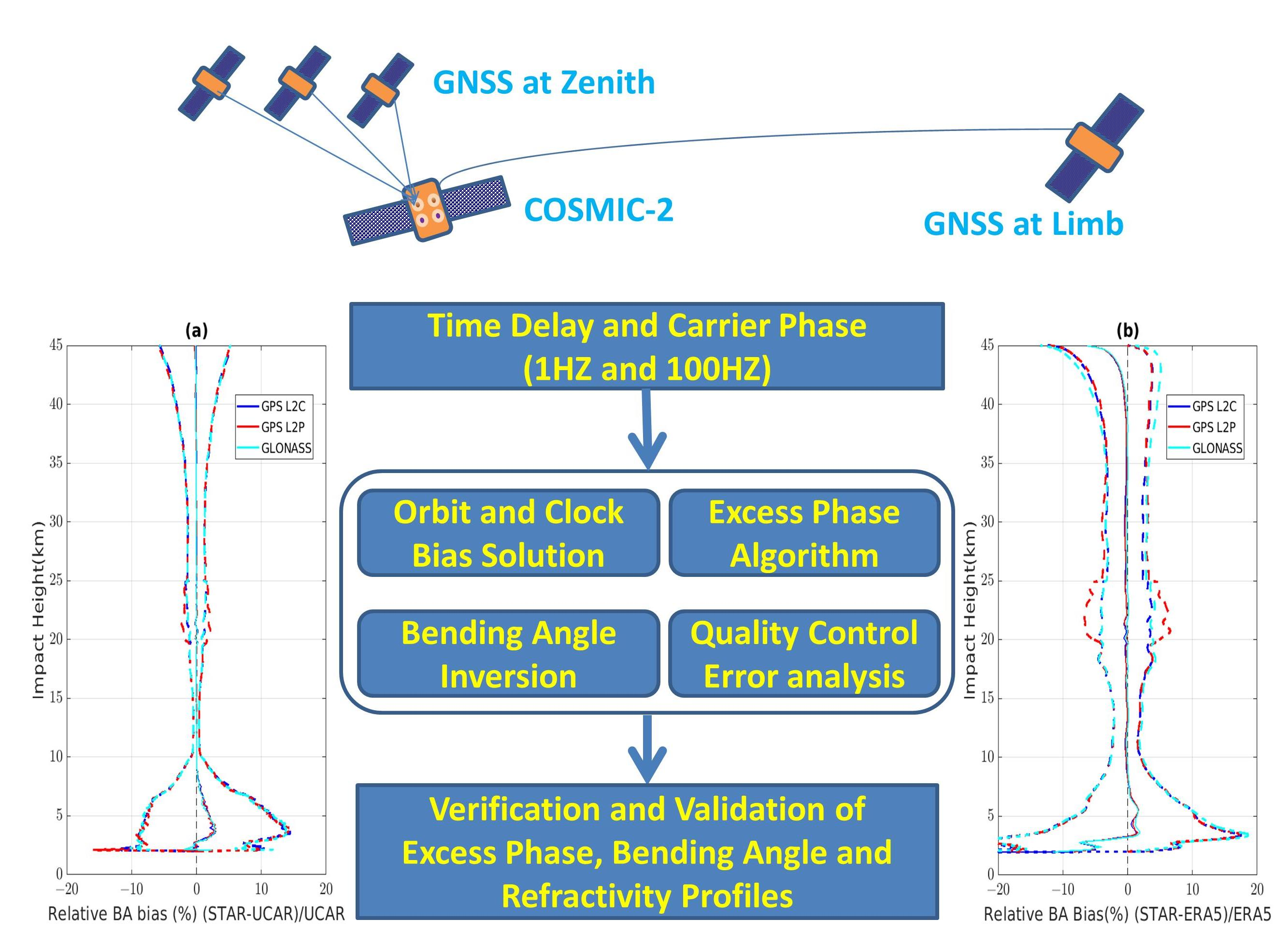
2. STAR Algorithms to Convert Carrier Phase to Excess Phase and Bending Angle Profiles

This section summarizes the initial COSMIC-2 data preparation and processing procedures to covert the COSMIC-2 carrier phase to the excess phase. Section 2.1 summarizes the flow chart for converting COSMIC-2 L0 data to L2 data products. Section 2.2 describes the initial preparation of COSMIC-2 L0 and L1a data for further processing. Section 2.3 describes the LEO receiver CLOCK bias estimation with POD. Section 2.4 presents COSMIC-2 excess phase calculation approaches, including carrier phase model description, receiver and transmitter clock bias correction, geometric range corrections, and phase error correction method. Section 2.5 describes how we use ROPP to convert COSMIC-2 excess phases to bending angle and refractivity profiles. Section 2.6 describes how we used the ERA5 dataset for validation/comparison.

2.1. Flow Chart for Converting COSMIC-2 L0 Observations to L2 Data Products

The flow chart for converting COSMIC-2 L0 observations to L2 data products at STAR is shown in Figure 2 (also see Figure 4 in [35]). Using a reading script provided by the UCAR CDAAC, we can decode the COSMIC-2 L0 data into L1a files, including the formatted carrier phase and pseudo-range measurements at a different rate for the POD antenna and occultation (OCC) antennas (Figure 2).

Table 1. STAR implementation of the RO processing chain.

Processing Step	Input Data	Main Output Data	Processing Methods/Libraries
Decoding L0 Data Set	COSMIC-2 L0 Datasets	COSMIC-2 L1a Dataset (opnGns and podCrx)	UCAR’s L0 to L1a Perl script
Extract RO events and pair with POD observations for reference GNSS satellite	OpnGns datasets podCrx datasets	Separate RO events and associated reference POD observation	opnGnss decoder (Perl) podCrx/RINEX reader, Matlab/IDL/bash scripts
The LEO Precise Orbit and Receiver Clock error estimation	COSMIC-2 Attitude Files; COSMIC-2 podCrx POD observations; CODE Final Orbital Products	COSMIC-2 POD (30 s, not used in this paper) and Receiver Clock bias at 2 s intervals (leoClk)	Bernese POD software Bash scripts for data preparation
GNSS/LEO Satellite Antenna Position (phase center), Geometric range calculation	CODE Final Orbit Products COSMIC-2 OpnGns and podCRX COSMIC-2 LeoOrb (UCAR), leoClk	GNSS/COSMIC-2 Position (ECI), Corrected receiver/transmitter time tag, the direct distance between GNSS/LEO.	GNSS Satellite Attitude Solution Model, GNSS transmitter position instrument ECEF/ECI conversion, Orbital polynomial interpolation, Signal propagation time calculation (Matlab)
COSMIC-2 receiver clock bias removal for excess phase calculation	COSMIC-2 carrier phase and receiver phase model(opnGns), 1 Hz POD observation (RINEX); Corrected receiver time tag, geometric range	Receiver clock bias and geometric range removed excess phase	Single differencing for ionospheric-free, position-free receiver clock bias calculation (Matlab); low pass filtering;
GNSS transmitter clock bias removal for excess phase calculation	Receiver Clock bias removed from the excess phase; Corrected transmitter time tag; CODE GNSS clock products	Receiver clock and GNSS clock bias and geometric range removed excess phase	Zero differencing; 4th Order polynomial interpolation (Matlab)
Excess Phase Cycle Slip correction and Navigation Bit Demodulation	Cleaned excess phase; GNSS navigation bit time series; Climatology (ROPP)	Cleaned excess phase	Multi-screen phase model with ROPP; Closed-loop cycle slip correction (Matlab); Open loop NDM and cycle slip correction with phase model (Matlab).
Other corrections	Receiver ambient multi-path; Phase wind up	Excess phase; corrected excess phase	Evaluated, not included.
Quality Control (Excess Phase)	Excess phase/position/time tag/SNR	NetCDF file with excess phase, transmitter/receiver position in ECI, receiver time tag in GPS seconds	Slight quality control, no output when excess phase not complete, e.g., broken time series.
Bending Angle Calculation	NetCDF with excess phase, positions, SNRs, and time tag	Bending angle/impact height, refractivity, the dry temperature at mean sea level, channels L1/L2, and optimal bending angle.	Interface implementation to ROPP
Quality Control (Bending Angle)	Bending angle/refractivity profiles	Quality flag (good/bad) insertion	Forward Operator using ROPP and ECMWF/ERA5, 15 sigma criteria in bending angle comparison.

summarizes the STAR RO L0-L2 implementations and specifies the input data and output products for each processing step (highlighted in Figure 2 as an orange box line). The input file format description can be found on the UCAR CDAAC website [39] and is not further detailed here.

2.2. Preparation of COSMIC-2 L0 and L1a Data

While COSMIC-1 POD has a 50 Hz sampling rate for reference for single differencing, the COSMIC-2 POD antenna only has a 1 Hz sampling rate. COSMIC-2 occultation (OCC) antenna also records the 100 Hz sampling rate, which is different from COSMIC-1. The high-rate OCC antenna observations are in the opnGns files (see Figure 2). The COSMIC-2 RO events can be easily separated based on the discontinuity in the measurements (say 30 s or longer) and tracking GNSS PRNs. Each GNSS satellite has an orbital period of about 12 h; the LEO satellite’s orbital period is usually less than 2 h. One OCC antenna can track only one GNSS satellite in its view zenith for a time window. The opnGns dataset includes the receiver time (as in GPS seconds since 1 January 1980, 00:00:00 UTC), the L1 and L2 carrier phase, the L1 phase model, the SNR, low rate (1 Hz) pseudo-range and range model, and tracking status (open loop or close loop). Like COSMIC-1, the COSMIC-2 phase model is provided only for L1. However, the phase model is provided for the whole profile in the COSMIC-2 data set. The COSMIC-2 attitude file follows the data format as CHAMP mission, where we can directly feed them into the Bernese GNSS software [40] for POD.

The GNSS ephemeris and clock information are needed for POD and excess phase calculation. We used the Center for Orbit Determination in Europe (CODE) GNSS final orbit products, which provide a 15 min resolution of GNSS orbits. Like the International GNSS Service (IGS), CODE can provide final, rapid, and ultra-rapid GNSS orbit products but with a different latency. Since we processed the COSMIC-2 datasets in a post-processed mode, we used the most accurate final CODE orbit solution, which usually has two weeks of latency but generally within 2 cm accuracy [41]. We also downloaded the 30 s GNSS CLOCK and the earth orientation information from the CODE website for COSMIC-2 POD and the excess phase calculation.

2.3. LEO Orbit and Receiver Clock Bias Determination

COSMIC-2 has two POD antennas. However, the front and rear antennas do not point to the zenith direction (against nadir) but at a tilted angle. Thus, the POD observed GNSS satellite could only be viewed in a cone in a rear or front direction. This reduces the total number of observations for one POD antenna compared to viewing the whole hemisphere when the antennas point to the zenith direction.

Here, we calculate the COSMIC-2 excess phase in a post-processing mode (two-week latency). We used the Bernese GNSS software to compute individual satellite POD and clock biases (Figure 3). The input parameters, GNSS final orbit, clock, and earth orientation products are from the CODE, and the attitude and RINEX files are from CDAAC. The COSMIC-2 clock bias solution is produced simultaneously with the orbital kinematic solution with every other observation epoch of 2 Hz. This clock bias is mainly used for correcting the time tag calculation (from the local receiver time to the GPS time) in the excess phase calculation.

COSMIC-2 clock bias is generally larger than COSMIC-1 (see Figure 3a–f). The receiver clock bias of COSMIC-1 is on the order of microsecond level (10⁻⁶ s) ([28]), and the clock stability (using Allan deviation to remove the time drift) of COSMIC ranges from 10⁻⁹ to 10⁻¹¹ over 1 to 104 s. Figure 3 depicts that the COSMIC-2 clock bias can be as large as a few milliseconds with a maximum drift of a few hundred microseconds per day. This requires a frequent clock bias adjustment to keep it within the millisecond range.

Figure 3g–l also show that COSMIC-2 clock drift is not stable. We removed the receiver clock bias in the excess phase using the single differencing method between POD and OCC observations. Currently, we used the POD solution from the UCAR data products as orbital inputs for the excess phase model. The GNSS orbital interpolation and LEO Clock solution (for excess phase time tag) are still from the output of the Bernese software.

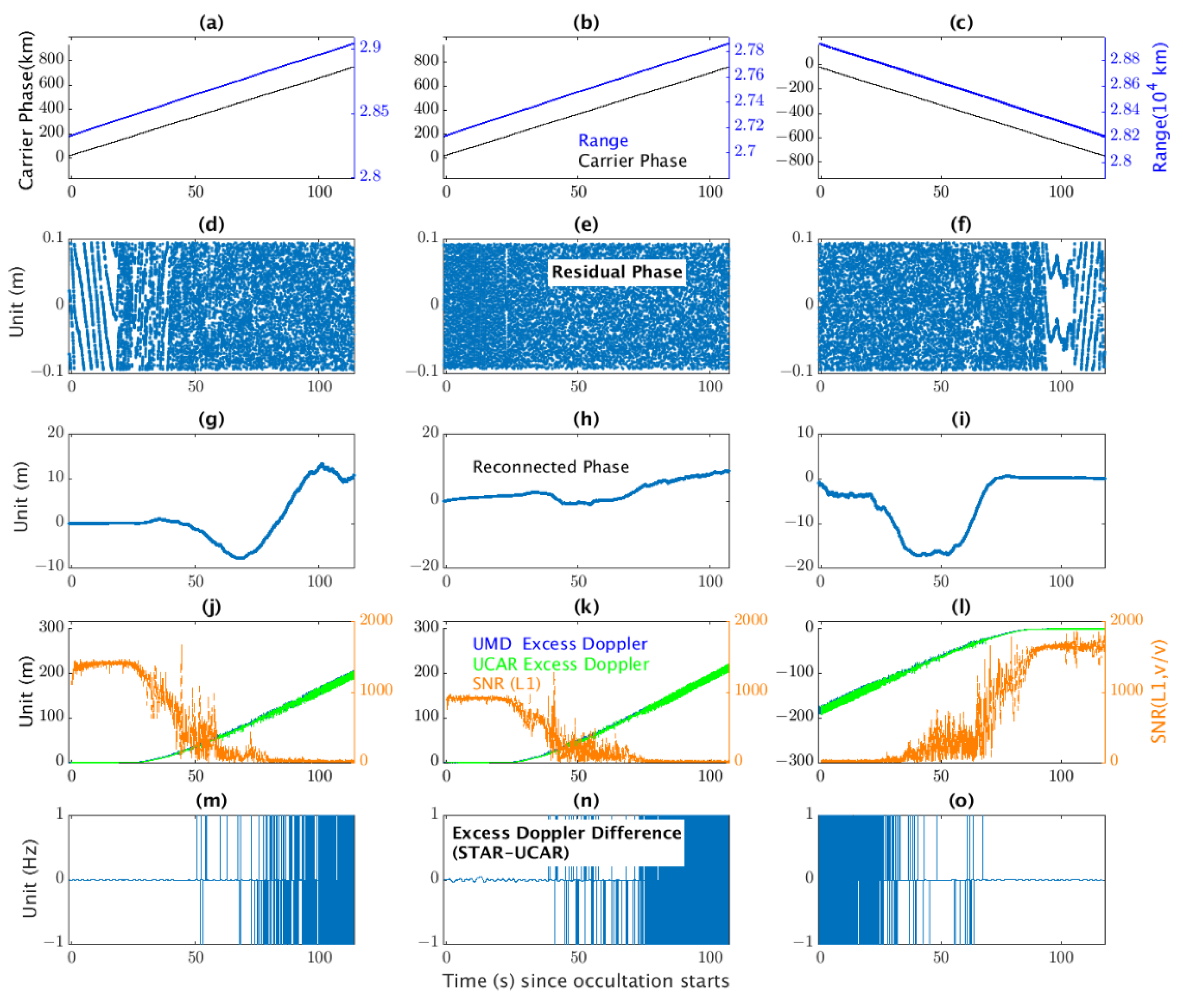
2.4. COSMIC-2 Excess Phase Calculation

2.4.1. Carrier Phase Model for Deriving the STAR COSMIC-2 Excess Phase

We derive the RO carrier phase equation using the wave propagation theory (see Appendix A). The derived carrier phase model (also see [25,42]) for retrieving the COSMIC-2 (and other RO missions) excess phase is

$$\begin{array}{ll}\hfill L_{LG}^F\left(t^R\left(t^{\prime }\right)\right)& =∆t^R\left(t^{\prime }\right)·C+{\delta }^R\left(t^{\prime }\right)·C-∆t^T\left(t^{″}-\tau \right)·C-{\delta }^T\left(t^{″}-\tau \right)·C\\ & +\Vert {\stackrel{\rightharpoonup }{x}}^R\left(t\right)-{\stackrel{\rightharpoonup }{x}}^T\left(t-\tau \right)\Vert +\delta D\left({\stackrel{\rightharpoonup }{x}}^R\left(t\right), {\stackrel{\rightharpoonup }{x}}^T\left(t-\tau \right)\right)+∆S+N+\in \end{array}$$

(1)

where t is the GPS time defined on the geoid surface on the earth, $L_{LG}^F\left(t^R\left(t^{\prime }\right)\right)$ is the observed carrier phase at local receiver time $t^R\left(t^{\prime }\right)$, $t^{\prime }$ is the proper time on the LEO orbit, $∆t^R\left(t^{\prime }\right)$ is the receiver (R) clock bias, $∆t^T\left(t^{″}-\tau \right)$ is the GNSS transmitter (T) clock bias, $t^{″}-\tau$ is the transmitter’s proper time at the signal transmitting, ${\delta }^T$ is the time correction from the local observer on earth geoid to proper time on orbit, ${\stackrel{\rightharpoonup }{x}}^R\left(t\right)$ is the receiver antenna position in ECI and ${\stackrel{\rightharpoonup }{x}}^T\left(t-\tau \right)$ is the transmitter antenna position in ECI. $\delta D({\stackrel{\rightharpoonup }{x}}^R(t), {\stackrel{\rightharpoonup }{x}}^T(t-\tau ))$ is a gravitational delay, N represents the ambiguity, $∆S$ represents the desired atmospheric delay (the excess phase), $\in$ represents errors from the multi-path from the ambient environment of the receiver or other sources.

The first two terms on the right represent the LEO clock error and corrections from local time to GPS time. The third and fourth terms are GNSS clock error and correction. The fifth and sixth terms are the range between GNSS/LEO and its correction due to gravitational delay, respectively. The eighth term is the phase ambiguity term. To estimate the excess phase $∆S$, we must first estimate each term in Equation (1) for L1 and L2 and GPS and GLONASS, respectively. The excess phase is calculated by removing the contributions from all these terms.

2.4.2. COSMIC-2 Receiver and GNSS Transmitter Clock Bias Removal

We used a coarse resolution of the receiver clock bias obtained from the COSMIC-2 POD solution to correct the carrier phase time tag. The POD receiver clock bias solution determines the true time approximately (with errors of equipment group delay) at antenna position for geometric range calculation and the interpolation for various analyses. During the excess phase calculation, the receiver clock bias from the POD solution is used to compute the coordinate time on orbit at which the receiver carrier phase was measured. Then, all the positioning, velocity, and carrier phase error removal will be based on this time. Given that the LEO satellite’s orbital movements are 7 km per second, the inaccurate time representation of 0.1 ms can yield the antenna position error of 70 cm (not POD error), much larger than the orbital requirement of 10 cm. This position error can be projected onto the time, phase, and Doppler frequency domain.

The accuracy of the bending angle derived from the excess phase is greatly affected by how the clock bias is effectively removed [25,28,43]. However, the receiver clock bias removal from the carrier phase needs to be re-determined in the excess phase calculation using single differencing for more accurate results (compared with the direct interpolation from the POD clock solution) given the significant clock bias of COSMIC-2. The single difference clock bias solution was derived using the paired observation from POD antennas’ reference link and different satellites’ occultation observations. The difference between the clock bias correction using the single differencing and Bernese LEO clock solution is 10⁻⁶ s level over the occultation periods (about 2–3 min).

COSMIC-1 has a high rate of reference link observations with 50 Hz on POD antennas. These observations from a GNSS satellite, usually in antenna zenith direction, can form an ionospheric free, distance free phase combined with the occultation phase measurement from another satellite, generally in a limb direction, to be used for the receiver clock removal for single differencing. Since there are no high-rate observations from COSMIC-2 POD antennas, one alternative is to use the low-rate RINEX observations with a sampling rate of 1 Hz. The linear combination of carrier phase L1 and L2 can be used as:

$$L_{L^{\prime }{G}^{\prime }}^3=L_{L^{\prime }{G}^{\prime }}^1+\frac{f_2^2}{f_1^2-f_2^2}\left(L_{L^{\prime }{G}^{\prime }}^1-L_{L^{\prime }{G}^{\prime }}^2\right)$$

(2)

where $L_{L^{\prime }{G}^{\prime }}^2$ is the L2 signal from GNSS G’ received by receiver L’, f1 and f2 are frequencies of the GNSS signal L1 and L2. This ionosphere-free L3 must also be geometric-free, where the direct distance between the POD antenna and the reference GNSS has been removed. Note that the frequency of each GLONASS constellation may be different. Some RINEX carrier phases display a jump every other epoch with less than around ¼ cycle. A low pass filter and reconnection of the residual phase from a polynomial fitting is used to remove the oscillation from the constructed L3, which otherwise will be introduced into the excess Doppler as noise.

The GPS time tag of the receiver observation (after correction) is also compared with that from UCAR. Generally, the difference is in the order of 10⁻⁷ s. This reflects the difference in receiver clock time calculation from UCAR. The magnitude of time tag difference on this level will not affect the later conversion from excess phase to bending angle since the clock bias is effectively removed using the single differencing method during the excess phase calculation.

The zero-differencing can also be used effectively to remove the clock bias if the clock bias can be accurately evaluated. All the time errors and corrections in the equation must be accounted for. COSMIC-2 satellites were designed with very stable atomic clocks. However, the clock bias calculated from Bernese GNSS software shows that the COSMIC-2 clock does not perform better than that of COSMIC-1. Figure 3g–l shows a considerable drift in the clock with a maximum rate of about 1–2 milliseconds/day. The significant clock bias can be effectively modeled and removed using a least-square polynomial curve fitting. The residual clock bias is comparable to the COSMIC-1. The excess phase/bending angle results using the single and zero differences are compared in Section 5.

The GNSS clocks bias (and drift) data can be downloaded from CODE products with a clock solution of 30 s. Considering the GNSS satellites’ extremely stable clock drift, a 4th order polynomial interpolation scheme has been used to estimate the GNSS clock bias in the excess phase calculation. These interpolations can still display a small discontinuity in the excess phase, which causes excess Doppler noise. This can bring more significant noise than UCAR operational products, where the double differencing with ground observations was used to remove the GNSS clock bias. However, this may only affect the bending angles at the upper altitudes, where very small bending angle values are located.

2.4.3. Geometric Range Corrections

Precise position estimates of the LEO and GNSS satellites are essential for accurate excess phase retrieval. The GNSS orbits were resampled using Bernese GNSS software from 15 min to 30 s through refitting its orbital dynamic parameters from CODE orbit solutions. These 30 s datasets are then used to calculate high-resolution GNSS satellite mass center position through polynomial interpolation (11th order) at the GNSS signal transmitting time. The clock bias results are simply polynomial interpolation of the CODE 30 s datasets.

The POD and clock bias for LEO and GNSS satellites are stored in the IGS Extended Standard Product 3 Orbit format (SP3-C). The receiver clock bias is used to convert the observation time on the local receiver time to the coordinate time. The corrected coordinate time is then used to calculate (interpolate) the LEO orbit in the ECI coordinate system. The antenna offset and the phase center variation has been converted from instrument coordinate to ECI using COSMIC-2 attitude files provided by UCAR. They were added to the mass center position (also converted to ECI) to retrieve the position and velocity. UCAR provides the COSMIC-2 attitude quaternions in a True of Epoch (TOE) ECI; we tested different ECI schemes. The difference between the TOE and other ECI for the antenna offset (usually less than a millimeter) can be ignored, given the antenna length of less than 1 m. For the GNSS satellite, the antenna parameters are obtained from the GNSS satellite parameter files (satellite.I14, PCV_COD.I14), which are updated online [44].

To calculate the direct link between the LEO satellite (RO antenna) and the GNSS satellite (transmitter antenna), the time delay τ of the ray path from the transmitter to the receiver in a vacuum needs to be calculated. The first guess is the interpolated GNSS antenna position at time t. A Newton’s relaxation method is applied to iterate the propagation time and the GNSS antenna position (with both updated in each iteration), given the initial positions of GNSS satellites at the observation time on the LEO receiver until the time delay is converged and the time difference between two iterate steps is less than ten ns. A preliminary evaluation of the excess phase (on the order of 6 km near-surface, corresponding to a 20 us time delay) has been used to count the time delay caused by the excess path. Given the converged time delay τ and the GNSS antenna position (and velocity), the direct link distance $\Vert {\stackrel{\rightharpoonup }{x}}^R(t)-{\stackrel{\rightharpoonup }{x}}^T(t-\tau )\Vert$ can be calculated at time t. The range correction term due to the relativistic effects $\delta D({\stackrel{\rightharpoonup }{x}}^R(t), {\stackrel{\rightharpoonup }{x}}^T(t-\tau ))$ ([25,42]) has also been considered, and the general magnitude is on the order of 0.2 m, which is nearly constant and has negligible effects on the excess phase.

The validation is carried out as the direct radial distance from the earth center or between the transmitter and receiver phase center is independent of the coordinate system. The direct antenna radial distance (from the earth center) is compared with that from UCAR, and the difference is generally within 20 cm, and the time variation can be neglected. Note that a direct comparison between antenna positions can yield a difference in the order of meters in ECI horizontal direction due to the different coordinate systems used. Sometimes, this can be more than meters due to POD differences, which have been discussed later in the discussion section.

2.4.4. Extra Excess Phase Error Corrections

The transmitted signal can have a phase difference from the actual path transmitted due to the relative rotation between the GNSS transmitter and the LEO receiver antenna and the nature of the GNSS microwave signals’ polarization. This phase change with the rotation angle cannot be attributed to the ambiguity. Wu et al. [45] calculated this phase difference for receivers on the ground stations. We must find the instrument coordinate system’s antenna dipole for the LEO satellite receivers. For COSMIC-2, the boresight vectors can be used for this. However, depending on the clock removal method, the phase windup caused by the receiver side dipole rotation is not included for the single differencing method. The phase variation has been largely absorbed into the receiver clock bias and can be removed through single differencing. This term is small and negligible for contributions from different GNSS satellites since the relative rotation between the GNSS and LEO satellites is approximately 2 h.

The multi-path from the receiver ambient is not corrected. A recent study shows that COSMIC-2 multi-path effects from spacecraft ambient environment are minor [46]. This multi-path is different from the atmospheric-caused multi-path, which can be partially resolved using wave optics methods in bending angle conversion. There is no bending angle derivation in the lower atmosphere because SNR values are too low to resolve that.

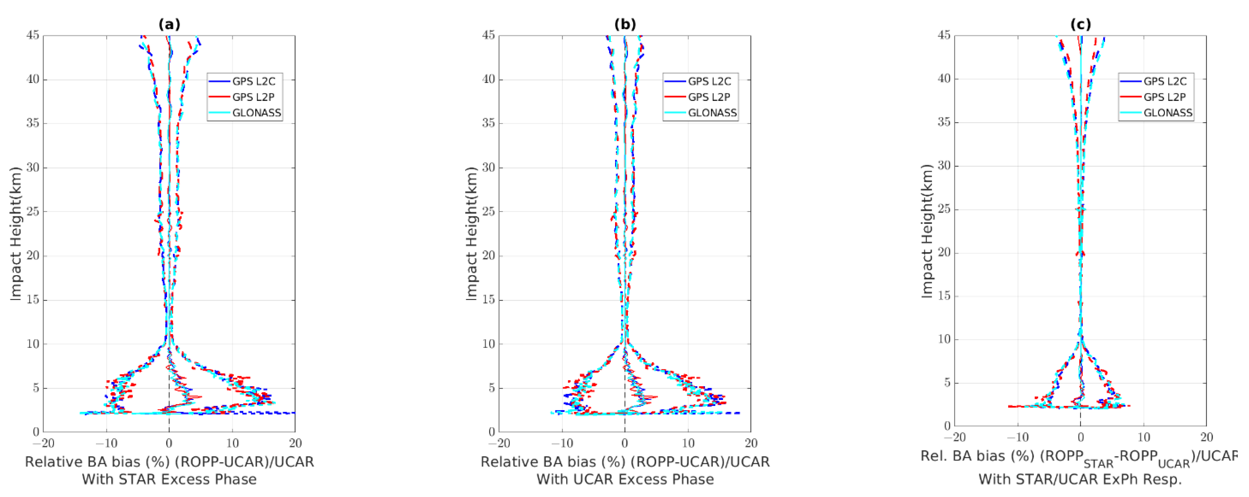
2.5. Using ROPP to Convert COSMIC-2 Excess Phases to Bending Angle Profiles and Refractivity Profiles

We used the ROPP-9.0 [37] to convert the excess phase to a bending angle. For lower atmosphere open-loop datasets with multi-path effects using wave optics (WO) retrievals, ROPP uses canonical transform of the second type (CT2) [47] to derive the bending angle from the excess phase. The CT2 approach is different from the Full Spectrum Inversion (FSI) method. While the FSI assumes a circular orbit for the satellites [33], the CT2 method incorporates the numerical efficiency of the FSI. It provides the most accurate results compared to other available bending angle inversion methods [32].

Note that because the ROPP-9.0 is not initially configured for COSMIC-2 data processing, we made some code changes to the package to include GPS and GLONASS for COSMIC-2 excess phase processing, with a similar configuration for applying ROPP to process COSMIC data.

The Mass Spectrometer and Incoherent Scatter Radar (MSIS) climatology dataset is used with ROPP for statistical optimization, excess phase model calculation, bending angles, and refractivity conversion. The Linear Abel integral method is used in Abel conversion in ROPP, assuming a linear variation of bending angle and refractivity logarithm. The statistical optimization method is used to derive an optimal bending angle. The vertical resolution of the output bending angle is interpolated to 100 m from the raw resolution. We extend the inversion to 150 km and keep the bending angle, refractivity, and dry temperature at the exact top height. Other parameters are kept the same as the default settings in the ROPP preprocessing package for the COSMIC-1 processing. The cut-off limits from impact height are −2 km, for the bending angle is 0.1, and the straight-line tangent altitude (SLTA) is −250 km.

In addition, we also modified the original ROPP codes to accommodate the COSMIC-2 high-rate occultation observations (100 Hz compared to COSMIC-1 50 Hz) and to include GLONASS observation signals. For GLONASS, the L1/L2 frequencies are different from GPS, and the navigation bit message 100 Hz is also different from GPS 50 Hz. This has been coded into the package. ROPP adopts a simple earth-centered inertial coordinate system, which only considers the mean sidereal time effects (Earth rotation). While the antenna velocity is provided with excess phase calculation, ROPP calculates the velocity internally from the position and time directly in ECI coordinates. We have generated the position and velocity data consistent with this ECI frame and input them into ROPP for bending angle inversion.

2.6. Using ERA5 Data for Validation

We use a BA forward operator to convert ERA5 temperature/water vapor profiles to bending angle profiles. Note that the COSMIC-2 RO data in this study had not been assimilated into ERA5 for the study period (October 2019). The RO assimilation to ECMWF was started a few months later, on 25 March 2020. The ERA5 datasets are used to simulate the bending angle profiles, which are used to validate the bending angle profile derived from the STAR RO processing package. The ERA5 temperature, pressure, and moisture are collocated with the bending angle profiles based on RO tangent point longitude, latitude, and the RO occultation time. Then, the collocated ERA5 datasets are linearly interpolated in space and time to match the bending angle profile. The spatially and temporally interpolated ERA5 datasets are then converted to refractivity using:

$$N=77.6\frac{P}{T}+3.73\times {10}^5\frac{e}{T^2}$$

(3)

where N is the refractivity to be calculated, P is the pressure and T is temperature, and e is the moisture vapor pressure.

Cubic spline vertical interpolation of the ERA5 profiles is carried out to get a finer resolution profile to reduce the vertical oscillation in bending angle. The super refraction points are firstly determined and removed from refractivity profiles. The forward operation uses composite Simpson’s integration of the Abel integral equation to convert refractivity to bending angle. The composite Simpson’s integration and the cubic vertical interpolation assure the smaller oscillation in the vertical integration of bending angle profiles than other tested schemes.

3. Verification of the STAR-Derived Excess Phase and Bending Angle Profiles

This section compares the STAR-derived COSMIC-2 excess phase, bending angle, and refractivity profiles to those derived from UCAR and forward simulations from ERA5.

3.1. Excess Phase Comparisons

Figure 4 shows three scenarios of different excess phase profiles processed from level 1a data (see Figure 2). Figure 4a–c depicts raw carrier phase time series from the opnGns files, which lasts about 2–3 min, corresponding to the GNSS satellite’s rising/setting time viewed from the LEO satellite. The difference (residual) between the calculated raw carrier phase and carrier phases model from receivers is provided in high-rate observations. Here, phase cycle slips can be seen clearly as the discontinuity from maxima to minima with two adjacent elements. These cycle slips are usually on a scale of a few wavelengths (e.g., 0.19 m for L1).

For L1, the method from [32] can effectively remove the cycle slips for high SNRs by checking the discontinuity in the phase difference (from the model) and restoring the phase continuity by adding integer numbers to the wavelength through minimization. However, there are still uncertainties in the lower troposphere, where atmospheric multi-path occurs. The residual phase time series can also be correlated with the GPS bit time series to remove additional cycle slips [48]. The cycle slip corrected residual carrier phases in our processing are added to the phase model to derive the excess phase for each frequency with clock bias correction and geometric range correction (Figure 4g–i). The excess Doppler is defined as the time derivatives of the excess phase. Figure 4j–l shows that the STAR excess Doppler (blue line) is of excellent agreement with those from UCAR (green line) for these three scenarios.

STAR-derived COSMIC-2 excess phases are very consistent with those derived from UCAR. Figure 5 compared the excess phases from STAR and UCAR for one day (~800 occultations) for C2E1 on 2 October 2019. The mean differences and standard deviations are 0.01 ± 0.04 m (Figure 5a) for rising profiles and −0.01 ± 0.03 m (Figure 5b) for setting profiles at 10 km, respectively. The close 0.2 m difference in the lower troposphere may be due to the remaining residual clock bias of some profiles. The mean difference and standard deviation increase below 10 km, where atmospheric multi-path effects occur. The excess phase difference increases dramatically below 10 km, indicating the cycle slip detection problem. Note that the excess phase is set to zero at the start time of setting or stop time of rising.

3.2. STAR Bending Angle Comparison with UCAR and ERA5

This study processed more than twelve thousand COSMIC-2 E1 occultation profiles collected in October 2019. Because all COSMIC-2 receivers (E1-E6) are of a similar quality (see [35]), we do not further repeat E2-E6 results hereafter.

The ERA5 temperature, moisture, and pressure profiles are interpolated onto the times and locations of COSMIC-2 data. The interpolated ERA5 datasets are then converted to bending angle profiles using the forward operator package described in Section 2.6. This section compares the STAR bending angle profiles with ERA5 and UCAR. STAR profiles passed quality control. (See Table 1) are used in the comparisons. We separate our comparisons with L2P/L2C signals and GPS/GLONASS satellites.

Figure 6a,b compared STAR-derived bending angle profiles with those from UCAR and ERA5 simulated bending angle profiles spatially and temporally collocated with COSMIC-2 events. The fractional bending angle difference (i.e., (STAR-ERA5)/ERA5 × 100%) is shown. Only “good” STAR-derived bending angle profiles are included in the comparison. The STAR-derived bending angle profiles are flagged as “bad” when the profile’s relative bending angle deviated from the background (ERA5 simulation) by more than 15 sigmas at any height below 45 km. For the STAR and ERA5 pairs, those profiles with more than 100% fractional differences at all altitudes below 60 km are excluded to derive the reference bias and standard deviation.

Figure 6a shows that the mean fractional bending angle difference between STAR and UCAR from 10 km to 35 km impact heights is less than 0.06%, and the standard deviation is less than 1.3%. However, a distinctive mean STAR-UCAR difference exists for L2P and L2C tracking signals. GPS L2P has a standard deviation of 1.32% (see

Table 2. Mean difference and standard deviation of bending angle and refractivity comparison with UCAR and ERA5 at 10–35 km.

Relative Percent (%)	GPS L2C		GPS L2P		GLONASS
	UCAR	ERA5	UCAR	ERA5	UCAR	ERA5
BA	−0.04 ± 1.15	−0.34 ± 2.96	−0.04 ± 1.32	−0.28 ± 3.81	−0.06 ± 1.15	−0.09 ± 3.20
Refractivity	−0.02 ± 0.83	−0.04 ± 1.06	−0.04 ± 0.97	0.09 ± 176	−0.05 ± 0.91	0.03 ± 1.08

). A relatively large STAR-UCAR standard deviation for GPS L2P compared to L2C occurred at impact heights from 20 km to 25 km.

The most significant standard deviation for L2C and GLONASS is 1.6% at 25 km impact height. The large standard deviation for the L2P profile mainly results from the considerable uncertainty in the raw L2P signals from those rising GPS satellites without L2C broadcasting [49]. The latest UCAR operational software has mitigated this issue (per communication with UCAR).

A good agreement in the monthly mean fractional bending angle profile between STAR and ERA5 is shown in Figure 6b. The mean fractional bending angle difference between heights 10–35 km is about −0.34 ± 2.96% for GPS L2C signals, −0.28 ± 3.81% for GPS L2P, and −0.09 ± 3.20% for GLONASS.

Generally, the STAR-ERA5 fractional bending angle difference and standard deviation (Figure 6b) are more significant than STAR-UCAR comparisons. At 5 km impact height, the mean fractional bending angle difference between STAR and ERA5 is 2%. The mean difference turns negative with decreasing altitude and fewer retrieved bending angle data points. For 8 km and below, a positive difference increases from 8 km to around 5 km.

While this positive fractional bending angle difference may be partially from the ROPP processing due to different configurations/parameterizations, the difference might be because the GNSS bit time series is not used for NDM removal. The internal bit removal process is suitable for large SNR values above 10 km with the phase model. Once it goes to the intensive cycle slip losing stage due to atmospheric multi-path effects and low SNR values, the ROPP’s internal NDM removal methods do not effectively remove the NDMs. This will slightly change the excess phase values toward the surface. In our processing, we plan to use the GNSS bit time series from other operational centers, such as UCAR or the EUMETSAT. The bending angle and refractivity mean difference and standard deviation compared with UCAR and ERA5 between 10 km and 30 km are also listed in Table 2.

3.3. Bending Angle Uncertainties Caused by Inversion Algorithm Implementation

To quantify the bending angle uncertainties caused by uncertainties in the excess phase, we compare the ROPP bending angle profiles while the excess phases are from (i) STAR and (ii) UCAR. We feed one day’s UCAR atmPhs (excess phase files) into ROPP to generate the bending angle profiles compared to those using STAR excess phase as inputs. Figure 7 compares these two bending angle profile sets with those from UCAR operational bending angle profiles. Figure 7a,b shows that the fractional bending angle profiles generally agree well with UCAR. The striking differences occur above 35 km and below 10 km for the double-difference using UCAR operational bending angle as transfers (Figure 7c). At upper altitude, the bending angle becomes very small, and a significant standard deviation in relative bending difference (about 5% at 45 km) can be related to the excess phase differences, which are mainly from the clock bias residual, POD effects, and excess phase profile smooth as discussed. However, excess phase differences cannot explain the relative bending angle differences of the lower atmosphere.

Below 10 km, the differences (to UCAR BA) are almost identical to the two ROPP results. There is a small zigzag structure below 4km and less than 5% STD error (increasing with lowering height), which might be related to the smoothing procedure in ROPP and the cycle slip removal procedure differences in the excess phase. Therefore, the ROPP algorithm setup can explain the difference below 10 km between UCAR bending angle and STAR bending angle profiles. As mentioned in previous sections, ROPP uses the MSIS climatology model as background from various corrections for the excess phase data and bending angle filtering. ROPP generates the excess phase model using input satellite parameters while examining the excess phase profiles for NDM removal and cycle slip corrections. The excess phase model is then used to unwrap the wrapped excess phase. The excess phase model difference from UCAR provides the main difference for the excess Doppler feeding into the CT2 routine for the bending angle conversion.

The ROPP algorithm caused bending angle difference from UCAR bending angle is similar to previous findings (e.g., ROM SAF with UCAR for Metop-A/B, [31]). To get a sense of how the ROPP bending angle inversion algorithm can cause the difference from the UCAR BA algorithm, we checked the comparison of ROM SAF reprocessed COSMIC-1 bending angle profile (more than 7000 profiles) in Jan 2016 by using the same excess phase from UCAR; thus, we can rule out the impacts of excess phase difference. The COSMIC-1 BA profiles comparison shows a similar pattern below 10 km, as shown in Figure 7b for COSMIC-2. Further examination shows that the excess phase model difference likely causes the main difference and different processing centers differentiate L2 processing. Discussion on the excess phase model will be another topic for further exploration.

3.4. Comparisons to UCAR Bending Angle for Different SNR Groups

Schreiner et al. [2] showed that the COSMIC-2 bending angle penetration depth is strongly correlated with the L1 SNR values at about 80 km altitude for GPS and GLONASS signals. The profiles can have a lower penetration depth approaching the surface with larger SNR values. Here, we analyze the SNR effects on our data comparison with UCAR results and examine how the SNRs affect RO processing. We adopted the UCAR convention, which uses SNR values at a high altitude of 80 km as references. In excess phase processing, the SNRs are correlated with the cycle slips. The larger the SNR values, the cycle slips can be quickly restored. At a low altitude below 10 km, cycle slips are strongly corrected with SNR values below 300 v/v.

Figure 8a compares the STAR processed bending angle with UCAR processed bending angle under different L1 SNR value categories. Clearly, the larger the SNR values, the better the comparison looks. There are relatively more significant standard deviations and larger wiggling structures in the bending angle difference/standard deviation profiles with lower SNR values. The standard deviation is the smallest for a group with SNR values >2000 v/v, both at high altitudes and near the surface. Additionally, the bias in this group is smaller, below 10 km, than in other groups. The worst case is for the lowest SNR groups, less than 500 v/v, with a more significant standard deviation and the most considerable difference below 10 km. The difference below 10 km for a group with <500 v/v indicates bending angle difference departure from UCAR occurs higher than in other groups, implying the SNRs values have impacted the penetration depth.

The significant variations of the SNR, as shown in Figure 8, can be associated with fluctuations in the excess phase. In Figure 3j–l, larger SNRs usually have fewer oscillations at the beginning (end) of setting (rising) occultation. The lower the SNR (at 80 km) is, the more quickly it approaches the large oscillation (large Scintillation index) region before becoming too weak to be used. Lower SNR values at 80 km mean the SNRs decrease rapidly over time. Gorbunov [50] has studied the SNR values with the RO inversion quality. There is no significant correlation between the SNR values and the bending angle quality unless the SNR value is too low and the bending angle profile cannot be correctly inverted. A detailed look at SNR values at the high altitude and the lower scintillation index may explain the difference since the SNR values can affect the cycle slip detection, especially the scintillation index, rather than the SNR values at high altitude.

The COSMIC-2 bending angle profiles penetration depth correlates with SNR values in the operational datasets, proving that larger SNRs can penetrate deeper [2]. This study can regenerate this correlation using the operational UCAR bending angle dataset and the STAR-generated bending angle profiles. While the correlation holds, a near-constant bias exists in the penetration depth across all SNR values between UCAR and STAR profiles (Figure 8b,c). This bias is around 0.55 km in mean sea level height and 0.4 km in impact height. While the excess phase profiles are generally the same in time (and hence straight-line height), the inversion to bending angle from modified ROPP determines the penetration depth. We also compared the correlation of penetration depth with L2 SNRs. Although a general correlation holds that larger SNRs correspond to deeper penetration depth, SNR L2 and penetration depth are less correlated with L2 SNR values higher than 600 v/v. This may be related to the SNR cut-off values used differently in this ROPP configuration and UCAR’s bending angle algorithm. L2 excess phase is processed differently than L1 in ROPP and UCAR bending angle conversions. At some low L2 SNR conditions, the lower part of the L2 is sometimes from extrapolation or simulation results. This is especially true for L2 SNRs. This is an interesting topic worthy of further exploration regarding the representativeness of the SNR at 80 km and the L2/L1 SNR differences.

3.5. Refractivity Comparison with UCAR and ERA5

The refractivity is a vertical Abel inversion from a bending angle as a function of impact height. All the bending angle errors can propagate into refractivity profiles and be amplified since they involve integration. Figure 9 shows the refractivity comparison for one month for C2E1 between UCAR and STAR profiles (Figure 9a) and ERA5 and STAR profiles (Figure 9b). The relative refractivity difference between STAR and ERA5 between 10 and 35 km is 0.09 ± 1.1%, 0.09 ± 1.9% for GPS L2P, and 0.06 ± 1.2% for GLONASS. The relative refractivity difference between STAR and UCAR between 10 km and 35 km is −0.02 ± 0.83%, −0.04 ± 0.97% for GPS L2P, and −0.05 ± 0.91% for GLONASS. The 10–35 km STAR profiles agree with ERA5 and UCAR refractivity results consistent with bending angle comparison. Compared with ERA5, the standard deviation of relative refractivity for rising GPS L2P signals is larger than other signals up to 45 km. In contrast, in bending angle profiles, the larger relative BA standard deviation for L2P occurs only between 20 and 25km, indicating the errors at a certain height level can propagate vertically through Abel inversion, which involves vertical integration of the bending angle.

4. Discussions

4.1. POD Uncertainties on the Excess Phase and Bending Angle Inversion

The requirements for COSMIC-2 POD are 10 cm. There are multiple POD solutions, sometimes as many as five, at a GPS epoch in the operational datasets. The multiple POD solutions in the operational POD generally match these requirements with a maximum difference of less than 10 cm; however, uncertainties exist from a few centimeters to meters. Using UCAR POD, the different solutions can affect the excess phase results, hence the bending angle. Figure 10 shows multiple POD operational products’ C2E1 mass center position radial difference. Most of the time, the POD differences are less than 10 cm. Sometimes it can be as high as a few meters. This is probably due to the different solutions from observation periods, POD antennas, or combinations of different signal systems (GPS/GLONASS).

For the excess phase calculation, the POD bias can be taken into excess phase calculation since the geometric distance between the POD antenna and the reference satellite transmitter antenna needs to be removed. Removing the single difference clock bias in the excess phase can also affect the L3 clock bias term. Using different POD solutions from operations, POD uncertainties can contribute to the excess phase difference (often as a trend, not a constant) and bending angle uncertainty. An example of the RO profiles under this condition is shown in Figure 10 using different POD results for a selected case: 18:46 UTC for G15 of C2E1. The changing satellite distance difference of 0.1 m in about 200 s (Figure 10a) is translated into excess phase (Figure 10b) about 0.25 m simultaneously. Here, the POD difference affects the calculated range between the GNSS satellite and RO antenna and the single differencing due to the direct link calculation between the LEO and referenced GNSS satellite. The bending angle difference at the upper altitude is significant in this situation, 10% different at 50 km (Figure 10c). Another scenario is when the two POD solutions are not on the same epoch but overlapped in time after the polynomial interpolation is applied to different POD solutions; the resulting antenna position difference can sometimes be even more than meter levels, affecting the excess phase and bending angle. This bending angle profile may be removed as outliers during the quality check, depending on the amplitude of the position error. This may be resolved during reprocessing using one day’s observations (longer arcs) to make the dynamic orbit fitting more accurate than hourly batches.

4.2. Zero Differencing versus Single Differencing

COSMIC-1 has high-rate linked datasets available, different from COSMIC-2. Generally, the single differencing from high-rate link observations is superior to the zero-differencing given the uncertainties in the Clock bias. While we present the results using single differencing for COSMIC-2, we have also tested the zero differencing results using POD resolved clock bias. There are uncertainties in the LEO clock errors due to less screening of the dataset. Noise in the clock solutions presents in the Bernese outputs (Figure 2). The single differencing requires the best reference GNSS satellite regarding SNR and GNSS satellite zenith. The signal delay between the POD and OCC antenna to the onboard central processing system might differ.

Figure 11 shows the bending angle difference using these two clock removal methods for 2 October 2019 for C2E1. Zero differencing can cause more considerable variations than UCAR towards the upper layer. This is understandable given that the UCAR datasets are also processed using the single differencing method. The zero differencing method did not consider the small corrections, such as the antenna signal delay differences, and the POD screening solution from Bernese may not completely remove those outliers since the Clock solution is not from the final kinematic screening, and hence noise in the clock bias evaluation can cause more significant deviations. The zero difference results can cause a 2% larger standard deviation of the relative bending angle at 35 km than single differencing results. However, the difference is usually a small addition in the Doppler domain; hence, it hardly affects the results at a lower altitude.

A low pass filter in the Doppler frequency domain is applied for the L3 ionosphere-free phase combination at a 1 Hz rate to remove the significant discontinuities and reintegrate them to form a smoothed L3. Moreover, the carrier phase ambiguity in the RINEX file (used for single differencing) must be removed. This can be further improved later, engaging in the Bernese software’s full usage for ambiguity solutions or other GNSS utility tools for carrier phase smoothing.

Carrier phase observations from multiple GNSS satellites can be used as the reference link for the single differencing clock bias removal. In our process, we have ensured that each RO event’s reference satellite has the highest SNR and high zenith angle viewed from the COSMIC-2 satellites. However, depending on the zenith angle, residual atmospheric delays can contaminate the clock bias solution when the zenith angle is away from 90°.

4.3. Setting and Rising Differences

UCAR bending angle shows a small setting and rising difference among the bending angle profiles compared with ECMWF and Met Office weather forecast results and other RO missions (Monthly comparison with ECMWF/Met Office model results from ROM SAF monitoring site: https://www.romsaf.org/monitoring/index.php, accessed on 4 July 2022) below 45 km. The mean difference is small, less than 0.5% at 55 km, and the standard deviation is consistent for rising and setting levels.

Figure 12 shows the STAR-derived bending angle compared with ERA5 in setting and rising conditions for 2 October 2019. Generally, there exists a setting/rising relative bending angle difference (from ERA5) separation above 35 km, and the separation can be significant at different times. The setting profiles tend to have a mean negative relative bias, while rising profiles have a positive mean bias, which can also be seen in the excess phase profiles. The standard deviation is nearly identical except for L2P rising. The relative difference gradually reduces towards the lower atmosphere. This bending angle difference comes from the residual bias difference in the excess phase from setting and rising profiles, which likely comes from the clock bias algorithm from a single differencing method or POD inconsistency used differently from operational products.

5. Conclusions

Given the uncertainty and error sources in processing raw phase to excess phase and satellite positioning/velocity, a comprehensive reprocessing from different centers using various algorithms is critical to access the structural uncertainty for COSMIC-2 data due to different inversion implementations (also see [51]). In this study, we presented the experiments of the STAR stand-alone procedures to convert the COSMIC-2 carrier phase to the excess phase and convert the excess phase to bending angle profiles. In this study, we analyzed possible errors during each step. We conclude our findings with the following:

(1)

While we use UCAR CDAAC’s COSMIC-2 Orbit solution, the receiver clock solution from the Bernese GNSS software is used as input for the excess phase calculation. The Bernese is also used as a tool for GNSS satellite orbital interpolation. However, the receiver clock bias removal in the excess phase is carried out with a single differencing method by differencing with the low rate (1 HZ) POD observations with proper reference satellite observations based on the SNR and zenith angle. We also tested the zero-differencing receiver bias clock removal method. We attributed the STD difference at high altitude from single differencing to large COSMIC-2 receiver clock bias, compared with the COSMIC-1 mission.

(2)

The comparison results show good agreement between STAR and UCAR excess phase above 10 km, and gradually, the mean difference and standard deviation increase below that level. There are setting and rising bias differences in the excess phase, reflecting differences in the bending angle conversion.

(3)

The ROPP package has been modified to accommodate the newly calculated COSMIC-2 excess phase from GPS and GLONASS. The results show excellent agreement in the relative bending angle compared with ERA5 simulated bending angle profiles and UCAR CDAAC bending angle profiles. Comparison with ERA5 shows that at the impact height of 10–35 km, the mean relative difference is about −0. 34 ± 2. 69% for GPS non-L2P signals, −0. 28 ± 3. 81% for GPS L2P, and −0.09 ± 3.20% for GLONASS. The difference below 8km gradually increases toward a maximum at 5km and decreases toward the surface. Above 35 km, there is an increase with altitude in relative bending angle standard deviation. The relative refractivity bears a similar feature with good agreement between 8 km and 35 km.

(4)

Compared with UCAR, from impact height of 10 km to 35 km, the mean relative difference is less than 0.06%. The standard deviation is usually less than 1.3%, and the difference for GPS L2P is also clearly relatively larger at heights 20–25 km. The GLONASS has a similar performance to the GPS L2C.

(5)

The L1 SNR value at 80 km is a good indicator of the strength of the GNSS signals transmitted. Comparison among the retrieval quality (comparison with UCAR) and the SNR values shows that the SNR values are correlated with the standard deviations and mean difference comparison with UCAR, implying the SNR impact on the RO bending angle inversion quality. We also found that L2 SNR at the same height (80 km) weakly correlates with the penetration depth only below 600 v/v.

(6)

While ROPP has been widely used for previous missions reprocessing by ROM SAF and some new missions, such as China’s GNOS FY−3 Fengyun mission, some improvements or modifications may be needed for the new mission. The bending angle algorithm difference between ROPP and UCAR can explain most lower troposphere differences. In contrast, the upper altitude difference is attributed to the excess phase algorithm regarding the clock bias removal, the ionospheric correction, and the positional errors, which are small but can be amplified due to the small bending angle comparison as the relative bending angle difference.

The produced datasets, including the excess phase and bending angle profiles, are available through the NOAA STAR Radio Occultation team ICVS Website (ICVS).

In this study, we have developed our radio occultation package to examine various error terms and their sources to understand better the RO inversion algorithm and RO data quality control. As a part of a future mission to improve the RO data quality, we will keep working on Bernese GNSS software for POD and dynamic orbital solution and validation, using ground observation for GNSS clock removal, further improvement in the receiver clock removal algorithm, resolving issues near the surface (open-loop phase model) using ROPP or STAR FSI algorithm with further improving the ROPP processing. We will also work on automating the RO processing and expanding the work to other RO missions, including GeoOptics, SPIRES, COSMIC-1, and KOMPSAT−5.

References

1. Ho, S.-P.; Zhou, X.; Shao, X.; Zhang, B.; Adhikari, L.; Kireev, S.; He, Y.; Yoe, J.G.; Xia-Serafino, W.; Lynch, E. Initial Assessment of the COSMIC-2/FORMOSAT-7 Neutral Atmosphere Data Quality in NESDIS/STAR Using In Situ and Satellite Data. Remote Sens. 2020, 12, 4099. [Google Scholar] [CrossRef]
2. Schreiner, W.S.; Weiss, J.P.; Anthes, R.A.; Braun, J.; Chu, V.; Fong, J.; Hunt, D.; Kuo, Y.H.; Meehan, T.; Serafino, W.; et al. COSMIC-2 Radio Occultation Constellation: First Results. Geophys. Res. Lett. 2020, 47, e2019GL086841. [Google Scholar] [CrossRef]
3. Ho, S.-P.; Yue, X.; Zeng, Z.; Ao, C.O.; Huang, C.-Y.; Kursinski, E.R.; Kuo, Y.-H. Applications of COSMIC Radio Occultation Data from the Troposphere to Ionosphere and Potential Impacts of COSMIC-2 Data. Bull. Am. Meteorol. Soc. 2014, 95, ES18–ES22. [Google Scholar] [CrossRef]
4. Ho, S.-P.; Peng, L.; Anthes, R.A.; Kuo, Y.-H.; Lin, H.-C. Marine Boundary Layer Heights and Their Longitudinal, Diurnal, and Interseasonal Variability in the Southeastern Pacific Using COSMIC, CALIOP, and Radiosonde Data. J. Clim. 2015, 28, 2856–2872. [Google Scholar] [CrossRef] [Green Version]
5. Ho, S.-P.; Peng, L.; Vömel, H. Characterization of the long-term radiosonde temperature biases in the upper troposphere and lower stratosphere using COSMIC and Metop-A/GRAS data from 2006 to 2014. Atmos. Chem. Phys. 2017, 17, 4493–4511. [Google Scholar] [CrossRef] [Green Version]
6. Ho, S.-P.; Peng, L.; Mears, C.; Anthes, R.A. Comparison of global observations and trends of total precipitable water derived from microwave radiometers and COSMIC radio occultation from 2006 to 2013. Atmos. Chem. Phys. 2018, 18, 259–274. [Google Scholar] [CrossRef] [Green Version]
7. Ho, S.-P.; Anthes, R.A.; Ao, C.O.; Healy, S.; Horanyi, A.; Hunt, D.; Mannucci, A.J.; Pedatella, N.; Randel, W.J.; Simmons, A.; et al. The COSMIC/FORMOSAT-3 Radio Occultation Mission after 12 Years: Accomplishments, Remaining Challenges, and Potential Impacts of COSMIC-2. Bull. Am. Meteorol. Soc. 2020, 101, E1107–E1136. [Google Scholar] [CrossRef] [Green Version]
8. Biondi, R.; Randel, W.J.; Ho, S.-P.; Neubert, T.; Syndergaard, S. Thermal structure of intense convective clouds derived from GPS radio occultations. Atmos. Chem. Phys. 2012, 12, 5309–5318. [Google Scholar] [CrossRef] [Green Version]
9. Biondi, R.; Ho, S.-P.; Randel, W.; Syndergaard, S.; Neubert, T. Tropical cyclone cloud-top height and vertical temperature structure detection using GPS radio occultation measurements. J. Geophys. Res. Atmos. 2013, 118, 5247–5259. [Google Scholar] [CrossRef]
10. Huang, C.Y.; Teng, W.H.; Ho, S.P.; Kuo, Y.H. Global variation of COSMIC precipitable water over land: Comparisons with ground-based GPS measurements and NCEP reanalyses. Geophys. Res. Lett. 2013, 40, 5327–5331. [Google Scholar] [CrossRef]
11. Teng, W.-H.; Huang, C.-Y.; Ho, S.-P.; Kuo, Y.-H.; Zhou, X.-J. Characteristics of global precipitable water in ENSO events revealed by COSMIC measurements. J. Geophys. Res. Atmos. 2013, 118, 8411–8425. [Google Scholar] [CrossRef]
12. Scherllin-Pirscher, B.; Kirchengast, G.; Steiner, A.K.; Kuo, Y.-H.; Foelsche, U. Quantifying uncertainty in climatological fields from GPS radio occultation: An empirical-analytical error model. Atmos. Meas. Tech. 2011, 4, 2019–2034. [Google Scholar] [CrossRef] [Green Version]
13. Zeng, Z.; Ho, S.-P.; Sokolovskiy, S.; Kuo, Y.-H. Structural evolution of the Madden-Julian Oscillation from COSMIC radio occultation data. J. Geophys. Res. Atmos. 2012, 117, D22108. [Google Scholar] [CrossRef]
14. Rieckh, T.; Anthes, R.; Randel, W.; Ho, S.-P.; Foelsche, U. Tropospheric dry layers in the tropical western Pacific: Comparisons of GPS radio occultation with multiple data sets. Atmos. Meas. Tech. 2017, 10, 1093–1110. [Google Scholar] [CrossRef] [Green Version]
15. Schröder, M.; Lockhoff, M.; Shi, L.; August, T.; Bennartz, R.; Brogniez, H.; Calbet, X.; Fell, F.; Forsythe, J.; Gambacorta, A.; et al. The GEWEX Water Vapor Assessment: Overview and Introduction to Results and Recommendations. Remote Sens. 2019, 11, 251. [Google Scholar] [CrossRef] [Green Version]
16. Xue, Y.; Li, J.; Menzel, W.P.; Borbas, E.; Ho, S.P.; Li, Z.; Li, J. Characteristics of Satellite Sampling Errors in Total Precipitable Water from SSMIS, HIRS, and COSMIC Observations. J. Geophys. Res. Atmos. 2019, 124, 6966–6981. [Google Scholar] [CrossRef] [Green Version]
17. Mears, C.; Ho, S.-P.; Wang, J.; Peng, L. Total Column Water Vapor, [In “States of the Climate in 2017”]. Bull. Amer. Meteor. Sci. 2018, 99, S26–S27. [Google Scholar] [CrossRef]
18. Mears, C.; Ho, S.-P.; Bock, O.; Zhou, X.; Nicolas, J. Total Column Water Vapor, [In “States of the Climate in 2018”]. Bull. Amer. Meteor. Sci. 2019, 100, S27–S28. [Google Scholar] [CrossRef] [Green Version]
19. Anthes, R.A.; Bernhardt, P.A.; Chen, Y.; Cucurull, L.; Dymond, K.F.; Ector, D.; Healy, S.B.; Ho, S.-P.; Hunt, D.C.; Kuo, Y.-H.; et al. The COSMIC/FORMOSAT-3 Mission: Early Results. Bull. Am. Meteorol. Soc. 2008, 89, 313–334. [Google Scholar] [CrossRef]
20. Syndergaard, S. On the ionosphere calibration in GPS radio occultation measurements. Radio Sci. 2000, 35, 865–883. [Google Scholar] [CrossRef]
21. Cardinali, C.; Healy, S. Impact of GPS radio occultation measurements in the ECMWF system using adjoint-based diagnostics. Q. J. R. Meteorol. Soc. 2014, 140, 2315–2320. [Google Scholar] [CrossRef]
22. Ruston, B.; Healy, S. Forecast Impact of FORMOSAT -7/ COSMIC -2 GNSS Radio Occultation Measurements. Atmos. Sci. Lett. 2021, 22, e1019. [Google Scholar] [CrossRef]
23. Kursinski, E.R.; Hajj, G.A.; Bertiger, W.I.; Leroy, S.S.; Meehan, T.K.; Romans, L.J.; Schofield, J.T.; McCleese, D.J.; Melbourne, W.G.; Thornton, C.L.; et al. Initial Results of Radio Occultation Observations of Earth’s Atmosphere Using the Global Positioning System. Science 1996, 271, 1107–1110. [Google Scholar] [CrossRef]
24. Kursinski, E.R.; Hajj, G.A.; Schofield, J.T.; Linfield, R.P.; Hardy, K.R. Observing Earth’s atmosphere with radio occultation measurements using the Global Positioning System. J. Geophys. Res. Atmos. 1997, 102, 23429–23465. [Google Scholar] [CrossRef]
25. Schreiner, W.; Rocken, C.; Sokolovskiy, S.; Hunt, D. Quality assessment of COSMIC/FORMOSAT-3 GPS radio occultation data derived from single- and double-difference atmospheric excess phase processing. GPS Solut. 2009, 14, 13–22. [Google Scholar] [CrossRef]
26. Hwang, C.; Tseng, T.-P.; Lin, T.; Švehla, D.; Schreiner, B. Precise orbit determination for the FORMOSAT-3/COSMIC satellite mission using GPS. J. Geod. 2008, 83, 477–489. [Google Scholar] [CrossRef]
27. Weiss, J.-P.; Hunt, D.; Schreiner, W.; VanHove, T.; Arnold, D.; Jaeggi, A. COSMIC-2 Precise Orbit Determination Results. In Proceedings of the EGU General Assembly 2020, Online, 4–8 May 2020. [Google Scholar]
28. Xia, P.; Ye, S.; Jiang, K.; Chen, D. Estimation and evaluation of COSMIC radio occultation excess phase using undifferenced measurements. Atmos. Meas. Tech. 2017, 10, 1813–1821. [Google Scholar] [CrossRef] [Green Version]
29. Wang, Y.; Yang, R.; Morton, Y.T. Kalman Filter-based Robust Closed-loop Carrier Tracking of Airborne GNSS Radio-Occultation Signals. IEEE Trans. Aerosp. Electron. Syst. 2020, 56, 3384–3393. [Google Scholar] [CrossRef]
30. Steiner, A.K.; Ladstädter, F.; Ao, C.O.; Gleisner, H.; Ho, S.-P.; Hunt, D.; Schmidt, T.; Foelsche, U.; Kirchengast, G.; Kuo, Y.-H.; et al. Consistency and structural uncertainty of multi-mission GPS radio occultation records. Atmos. Meas. Tech. 2020, 13, 2547–2575. [Google Scholar] [CrossRef]
31. Xu, X.; Zou, X. Comparison of MetOp-A/-B GRAS radio occultation data processed by CDAAC and ROM. GPS Solut. 2020, 24, 34. [Google Scholar] [CrossRef]
32. Gorbunov, M.E.; Shmakov, A.V.; Leroy, S.S.; Lauritsen, K.B. COSMIC Radio Occultation Processing: Cross-Center Comparison and Validation. J. Atmos. Ocean. Technol. 2011, 28, 737–751. [Google Scholar] [CrossRef]
33. Adhikari, L.; Ho, S.-P.; Zhou, X. Inverting COSMIC-2 Phase Data to Bending Angle and Refractivity Profiles Using the Full Spectrum Inversion Method. Remote Sens. 2021, 13, 1793. [Google Scholar] [CrossRef]
34. UCAR COSMIC Program, COSMIC-2 Data Products (Level0, Level 1a and Level1b). Available online: https://www.cosmic.ucar.edu/what-we-do/cosmic-2/data (accessed on 16 June 2022).
35. Ho, S.-P.; Sho, X.; Chen, Y.; Zhang, B.; Adhikari, L.; Zhou, X. NESDIS STAR GNSS RO Processing, Validation, and Monitoring System: Initial Validation of the STAR COSMIC-2 Data Products. TAO COSMIC-2 Spec. Issue 2022. [Google Scholar]
36. Steiner, A.K.; Hunt, D.; Ho, S.P.; Kirchengast, G.; Mannucci, A.J.; Scherllin-Pirscher, B.; Gleisner, H.; von Engeln, A.; Schmidt, T.; Ao, C.; et al. Quantification of structural uncertainty in climate data records from GPS radio occultation. Atmos. Chem. Phys. 2013, 13, 1469–1484. [Google Scholar] [CrossRef] [Green Version]
37. Culverwell, I.D.; Lewis, H.W.; Offiler, D.; Marquardt, C.; Burrows, C.P. The Radio Occultation Processing Package, ROPP. Atmos. Meas. Tech. 2015, 8, 1887–1899. [Google Scholar] [CrossRef] [Green Version]
38. Liao, M.; Healy, S.; Zhang, P. Processing and quality control of FY-3C GNOS data used in numerical weather prediction applications. Atmos. Meas. Tech. 2019, 12, 2679–2692. [Google Scholar] [CrossRef] [Green Version]
39. UCAR/CDAAC RO Operational Data File Name Convention. Available online: https://cdaac-www.cosmic.ucar.edu/cdaac/doc/formats.html (accessed on 16 June 2022).
40. Dach, R.; Lutz, S.; Walser, P.; Fridez, P. (Eds.) Bernese GNSS Software Version 5.2. User Manual; Publikation Digital AG: Biel, Switzerland, 2015. [Google Scholar]
41. Dach, R.; Schaer, S.; Arnold, D.; Orliac, E.; Prange, L.; Susnik, A.; Villiger, A.; Jäggi, A. CODE Final Product Series for the IGS. 2016. Available online: http://ftp.aiub.unibe.ch/CODE/ (accessed on 4 July 2022).
42. Hajj, G.A.; Kursinski, E.R.; Romans, L.J.; Bertiger, W.I.; Leroy, S.S. A technical description of atmospheric sounding by GPS occultation. J. Atmos. Sol. -Terr. Phys. 2002, 64, 451–469. [Google Scholar] [CrossRef]
43. Wickert, J.; Beyerle, G.; Hajj, G.A.; Schwieger, V.; Reigber, C. GPS radio occultation with CHAMP: Atmospheric profiling utilizing the space-based single difference technique. Geophys. Res. Lett. 2002, 29, 28-21–28-24. [Google Scholar] [CrossRef] [Green Version]
44. Bernese GNSS Satellite Information, Problem and Phase Center Correction Files. Available online: ftp://ftp.aiub.unibe.ch/BSWUSER52/GEN (accessed on 16 June 2022).
45. Wu, J.; Wu, S.; Hajj, G.; Bertiger, W.; Lichten, S. Effects of antenna orientation on GPS carrier phase measurements. Manuscr. Geod. 1993, 18, 91–98. [Google Scholar]
46. Pedatella, N.M.; Zakharenkova, I.; Braun, J.J.; Cherniak, I.; Hunt, D.; Schreiner, W.S.; Straus, P.R.; Valant-Weiss, B.L.; Vanhove, T.; Weiss, J.; et al. Processing and Validation of FORMOSAT-7/COSMIC-2 GPS Total Electron Content Observations. Radio Sci. 2021, 56, e2021RS007267. [Google Scholar] [CrossRef]
47. Gorbunov, M.E.; Lauritsen, K.B. Analysis of wave fields by Fourier integral operators and their application for radio occultations. Radio Sci. 2004, 39, RS4010. [Google Scholar] [CrossRef]
48. Sokolovskiy, S.; Rocken, C.; Schreiner, W.; Hunt, D.; Johnson, J. Postprocessing of L1 GPS radio occultation signals recorded in open-loop mode. Radio Sci. 2009, 44, RS2002. [Google Scholar] [CrossRef]
49. FORMOSAT-7/COSMIC-2 Neutral Atmosphere Provisional Data Release 1. Available online: https://data.cosmic.ucar.edu/gnss-ro/cosmic2/provisional/F7C2_NA_Provisional_Data_Release_1_Memo.pdf (accessed on 16 June 2022).
50. Gorbunov, M. The influence of the signal-to-noise ratio upon radio occultation inversion quality. Atmos. Meas. Tech. Discuss. 2020, 2020, 1–11. [Google Scholar] [CrossRef] [Green Version]
51. Ho, S.-P.; Hunt, D.; Steiner, A.K.; Mannucci, A.J.; Kirchengast, G.; Gleisner, H.; Heise, S.; von Engeln, A.; Marquardt, C.; Sokolovskiy, S.; et al. Reproducibility of GPS radio occultation data for climate monitoring: Profile-to-profile inter-comparison of CHAMP climate records 2002 to 2008 from six data centers. J. Geophys. Res. Atmos. 2012, 117, D18111. [Google Scholar] [CrossRef]
Figure 1. The steps to convert RO from L0 data to L1 excess phase and converting excess phase to bending angle (L2) processing.
Remotesensing 14 03288 g001
Figure 2. STAR RO COSMIC-2 processing procedure. Different data product levels (level 0 to level 2) are also shown using the UCAR naming convention.
Remotesensing 14 03288 g002
Figure 3. COSMIC-2 FM1-FM6 clock bias and drift time series in October 2019. The left panel (af) shows COSMIC-2 Clock Bias (millisecond) from Bernese for 6 COSMIC-2 satellites, and the right panel (gl) shows the clock drift rate (millisecond/day, non-smooth, time derivative from clock bias) derived from the clock bias.
Remotesensing 14 03288 g003
Figure 4. From carrier phase to excess phase conversion with three scenarios of C2E1 (left: GPS setting for G14 at 2019.275 01:43:00 middle: GLONASS setting for R20 at 2019.275 11:31; Right: GPS rising for G09 at 2019.275 11:08). The top row (ac) shows the raw carrier phase (black line) and the calculated range (direct distance) between the GNSS satellite and the LEO satellite (blue line) for three cases. The second row (df) shows the phase residual (carrier phase minus receiver phase model) before cycle slip removal. The third row (gi) shows the residual excess phase after cycle slip removal. The fourth row (jl) shows the excess Doppler (black line represents STAR results, green lines are UCAR results) and L1 SNR (Unit: v/v) (orange lines). The fifth row (mo) shows excess Doppler differences.
Remotesensing 14 03288 g004
Figure 5. Excess Phase comparison between STAR and UCAR results (STAR-UCAR) for (a) rising and (b) setting for day 2019.275. The impact height is derived based on the geo-optical method from L1. The Solid line represents difference, and the dashed line represents standard deviation.
Remotesensing 14 03288 g005
Figure 6. (a) Relative bending angle profiles compared with UCAR results and (b) ERA5 simulated results over October 2019. The profile is grouped as GLONASS L2C (cyan), GPS L2C/L2L (blue), and GPS L2P (red). The solid line represents the relative difference, and the dashed line is the standard deviation. The waggling structure compared with ERA5 is due to the forward operator from refractivity to bending angle calculation using Abel inversion.
Remotesensing 14 03288 g006
Figure 7. ROPP inverted bending angle profile comparison with UCAR bending angle profiles using (a) STAR derived excess phase, (b) UCAR provided excess phase, and (c) profile differences statistics (STAR).
Remotesensing 14 03288 g007
Figure 8. STAR bending angle relative bias compared with UCAR are grouped with SNR values at 80 km impact height ((a), L2C only). (b) and (c) show the RO penetration depth of STAR and UCAR (green) related to L1 (b) and L2 SNR (c).
Remotesensing 14 03288 g008
Figure 9. Refractivity Comparisons with (a) UCAR and (b) ERA5.
Remotesensing 14 03288 g009
Figure 10. Using different POD solutions can yield different bending angle profiles. The POD difference (a) is up to 50 cm and changes with time for the case: 2 October 2019, 18:46 UTC for G15 of C2E1. The jump in the excess phase (b) is due to the cycle slip removal difference. The relative bending angle bias (c) can be about 10% around 50 km.
Remotesensing 14 03288 g010
Figure 11. Bending angle comparison with UCAR for 2019.275, for all non-L2P observation profiles, the outer envelope indicates one standard deviation; the middle two lines indicate relative differences. The green color represents the results of a single differencing, and the blue color for zero differencing.
Remotesensing 14 03288 g011
Figure 12. Bending angle comparison with ERA5 as setting and rising profiles for October 2019. The middle lines are mean relative differences, with standard deviation as outer lines. Red is for L2P rising, blue is for L2P setting, and green is for L2C (GPS and GLONASS). Profiles exceeding 10 sigmas at a height between 10 and 45 km have been removed in the comparison.
Remotesensing 14 03288 g012