4.1. Near-Field Experiment
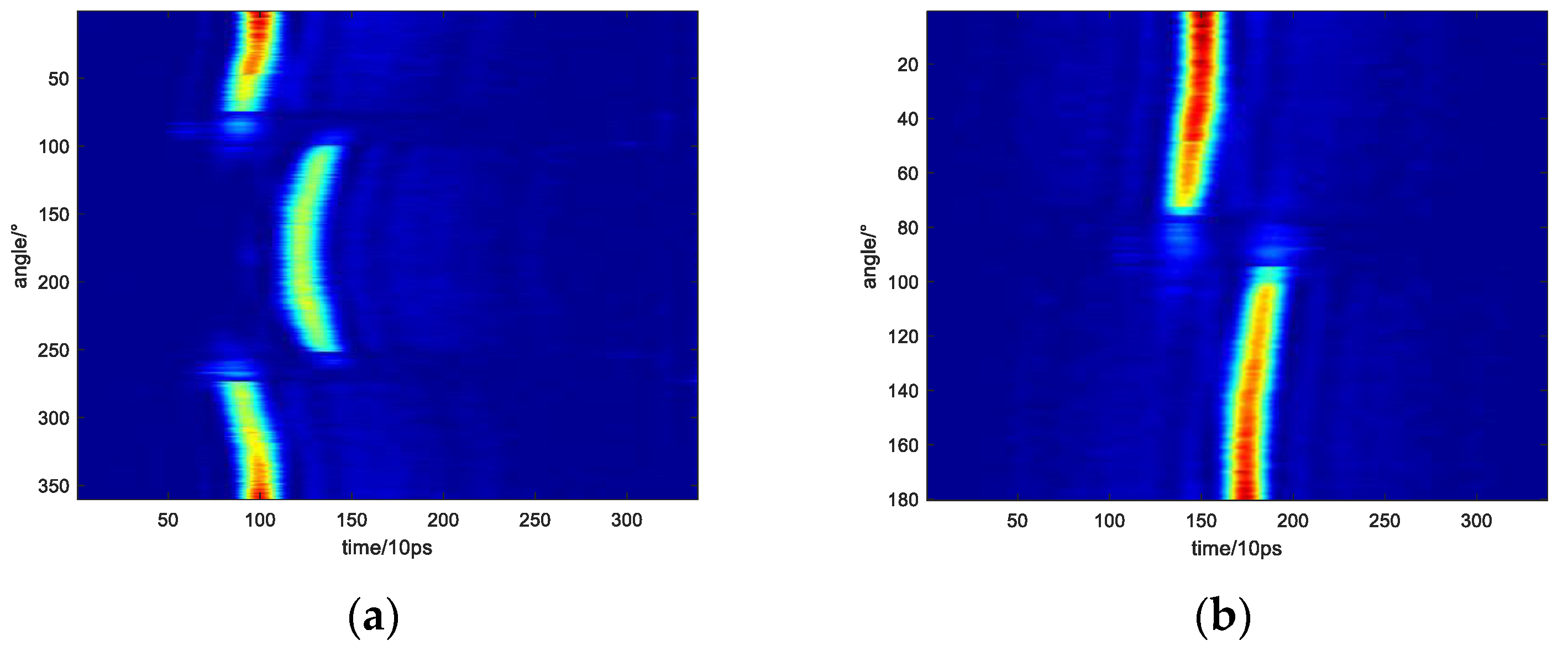
Figure 6a shows the laser reflection projection data after registration in the near-field experiment. A small amount of negative data is caused by the negative noise of the detector, so the negative value in the echo is eliminated. Then, the projection data are converted according to Equation (3), as shown in
Figure 6b.
For the projection data in the near-field experiment, the proposed TV sparse imaging reconstruction method in
Section 3.2 is performed compared with FBP [
10,
11,
12,
13], ART [
14], and sparse ART with a complete view of projections and uniformly sampled projections in 5°, 10°, and 20° viewing intervals. The results are shown in
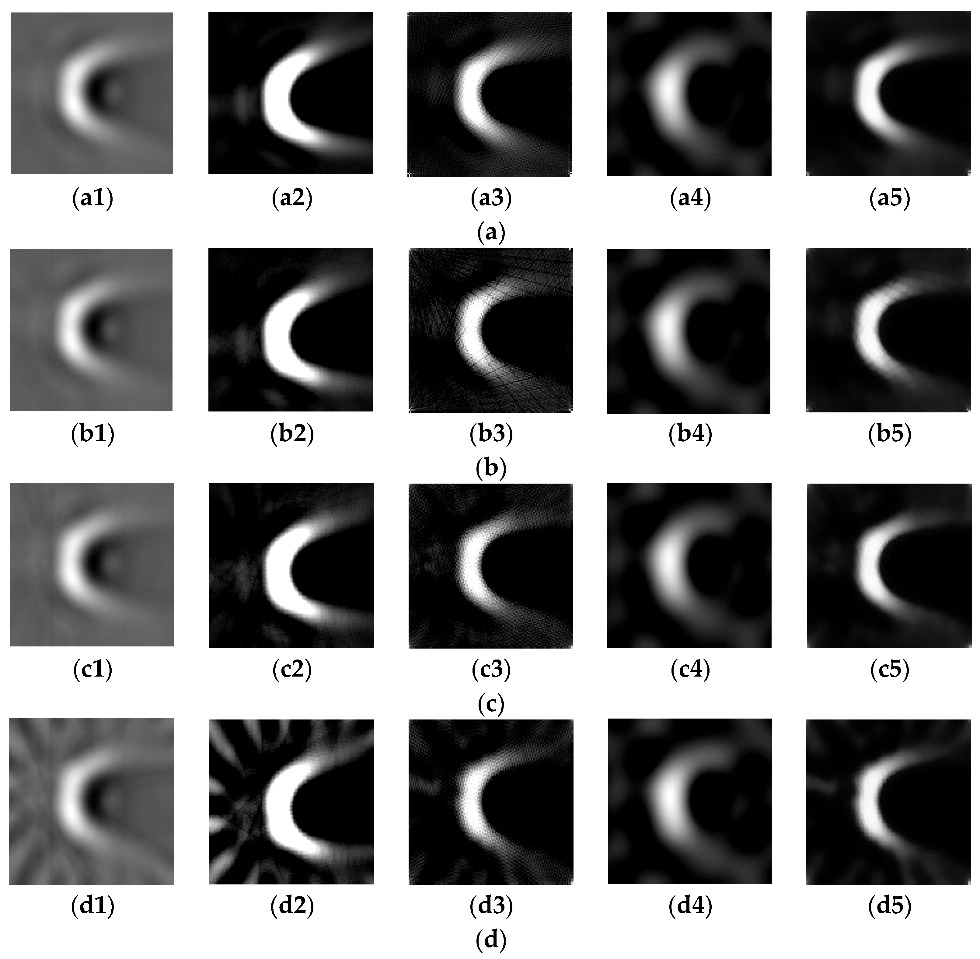
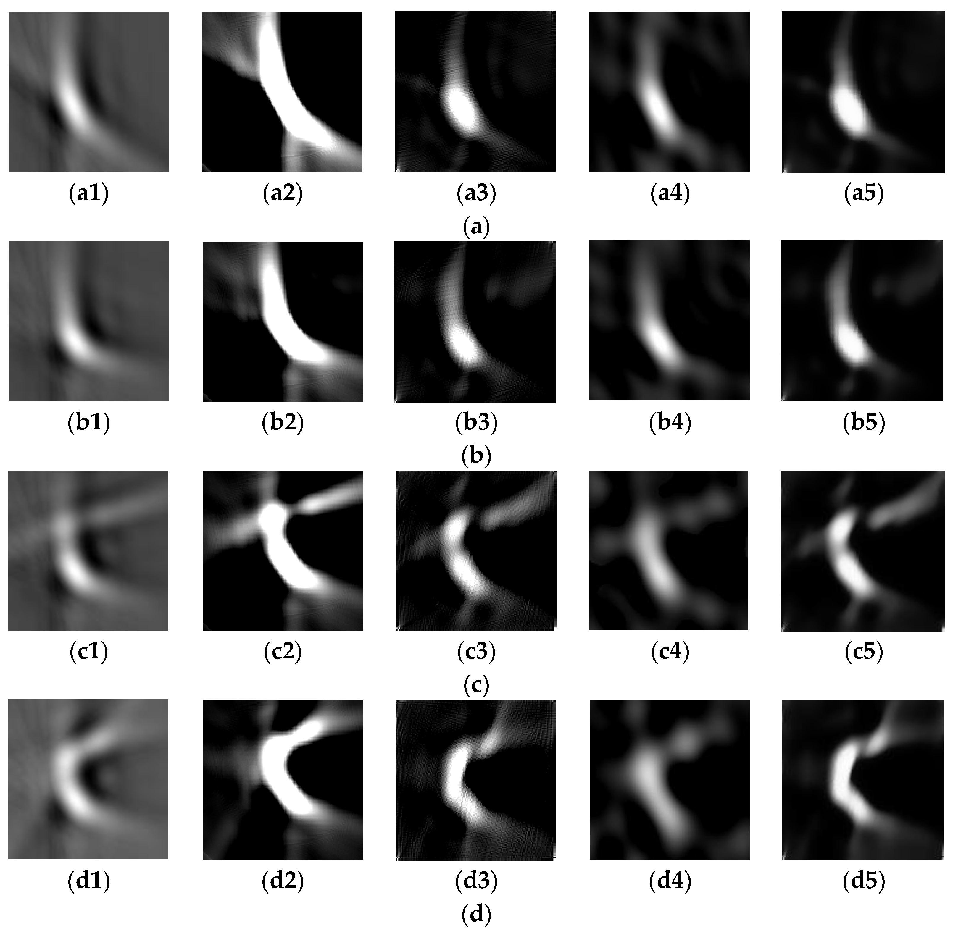
Figure 7. In
Figure 7a, the iRadon [
3,
9] results are illustrated just to show the target contour according to the definition in Equation (1), as mentioned in
Section 3.1. In
Figure 7(a4), for sparse ART with OMP algorithm mentioned in
Section 3.2.2, because of using discrete Fourier transform as a sparse basis, it cannot make good use of the gradient sparse features of laser image, leading to obvious deviation between the reconstructed contour and the original target. Then, for
Figure 7(a2,a3,a5), the target contour is very clear after imaging with all three approaches. In
Figure 7(a5), the resolution of the reconstructed image is significantly improved by using the proposed algorithm compared to
Figure 7(a2). Comparing
Figure 7(a5) with
Figure 7(a3), there are artifacts in the image reconstructed by the traditional ART, which are mostly eliminated in the result of the proposed method. Therefore, in the case of the complete angle, the proposed algorithm greatly improves the resolution of the reconstructed image and reduces the image artifacts.
Next, experiments are carried out at projections with viewing intervals of 5°, 10°, and 20°, respectively. In the near-field experiment, according to the Nyquist sampling theorem, the maximum projection angle sampling interval required to completely reconstruct the detected target laser image within the range of 360° is calculated as about 9°. In
Figure 7b, the sampling rate still meets the Nyquist sampling law, and the reconstruction result shows little difference from
Figure 7a. When the viewing interval of the projection data is 10° and 20°, the sampling does not meet the Nyquist sampling law. It can be noticed in
Figure 7c,d, with the increase in sampling angle interval, that the artifacts in the reconstructed image by iRadon and FBP algorithm increase significantly, which seriously affects the identification of the target contour. However, in the three results related to the ART in
Figure 7(c3–c5) and
Figure 7(d3–d5), the artifacts are in good condition. At the same time, the imaging resolution of the proposed algorithm is better than the traditional ART and sparse ART with the OMP algorithm. Comparing
Figure 7(d5) with
Figure 7(a5,b5,c5), with the increase in the sparsity of the angle, the image resolution is generally consistent with that in the complete angle. Furthermore, the artifact is in good condition and the image edge is smooth as well, which greatly reduces the requirements for the detection angle of non-conforming targets and provides convenience for high-efficiency and high-precision laser image reconstruction of non-conforming targets.
For quantitative assessment, information entropy (IE), no-reference signal-to-noise ratio (NRSNR), and variance (Var) are introduced to evaluate the imaging results by using different approaches. IE is defined as follows [
26,
27]:
where
is the probability that the pixel value in the image is
. According to Shannon’s information theory, larger entropy indicates more information. That is, the image is clearer with larger IE in LRT reconstruction.
SNR is the proportion of signal to noise and reflects the influence of the noise to signal or image. Here, the NRSNR is adopted to measure the denoising and artifact elimination effect of different reconstruction algorithms. Furthermore, the NRSNR is represented as follows [
28]:
where
is the noise level of the image,
is the noise distribution,
is the pixel value of the image,
is a set threshold, and
and
are the size of the image. The impact of the noise is smaller when the NRSNR value is higher, which indicates that the quality of the image is better. In this article, NRSNR is utilized to evaluate the anti-noise performance of different algorithms particularly.
Var reflects the contrast ratio of the image [
26], and the definition of Var is:
where
is the pixel value of the image at coordinates
and
is the mean pixel value of the whole image. In other words, it is easier to distinguish different objects when the Var is higher.
Based on the metrics mentioned above, all the reconstructed results in
Figure 7 are measured by IE, SNR, and Var as illustrated in
Table 1. As shown in
Table 1, the IE value of the TV sparse reconstruction method is the highest and maintains well at different sampling intervals, which indicates that the reconstructed image of the proposed method better reflects the feature of the target. Meanwhile, the SNR value and Var value of the proposed method are also better than the other algorithms at different sampling intervals, which further proves the effectiveness of the TV sparse reconstruction method in LRT.
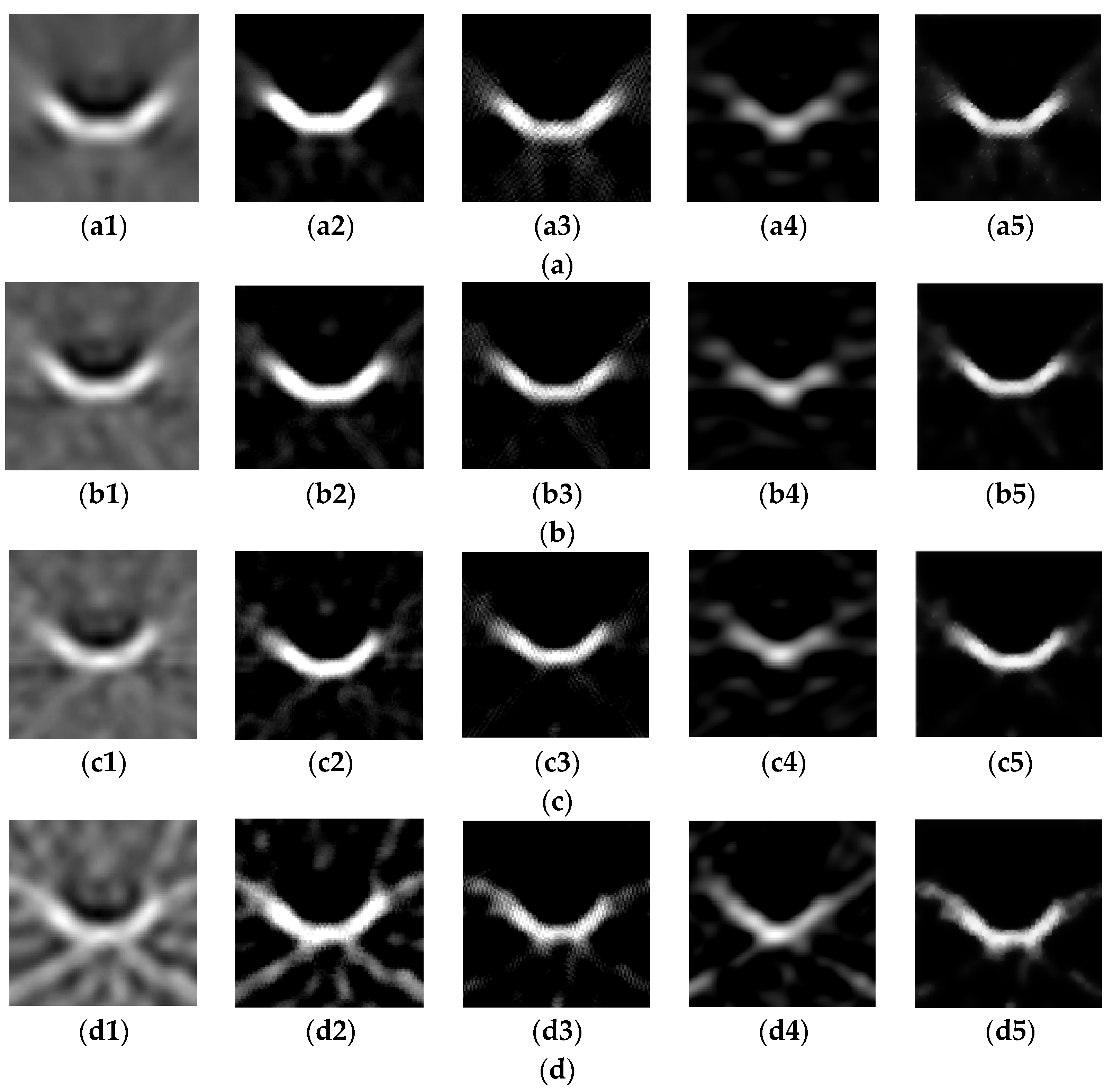
Then, we test the anti-noise performance of the proposed algorithm and explore if it still works under non-uniformly sampled projection data. Adding Gaussian noise to the projection data at complete view angles and 10° intervals, the images reconstructed by iRadon and FBP algorithm are destroyed by the noise in
Figure 8b, yet the proposed algorithm shows excellent performance in denoising regardless of the angle in
Figure 8(b5). It also performs better than the traditional ART not only in denoising ability but also in edge preservation. In addition, experiments are conducted in random sampling at 10° intervals, as shown in
Figure 8c. The result of the proposed algorithm in
Figure 8(c5) is superior to other algorithms in artifact elimination and the image can also be generally well reconstructed under the influence of random sampling. For better analysis, all the reconstructed results are evaluated by IE, NRSNR, and Var, illustrated in
Table 2. It can be concluded from
Table 2 that whether the projection data are added with noise or non-uniformly sampled, the IE and Var of the proposed method are still better than that of the other three. It also can be noted that the NRSNR of the reconstructed image using the proposed method is 2.2245 and 2.5897 in complete views and 10° intervals, respectively, almost 30% higher than that of the FBP, ART, and OMP approaches, which highlights the anti-noise performance of the TV sparse reconstruction method with incomplete views of projection data.
Finally, the proposed algorithm is tested under 0–60°, 90°, 120°, and 150° views of projections. Among the results, the image can be roughly reconstructed under the 150° view of projections, as shown in
Figure 9c, and
Figure 9(c5) shows that the resolution under the proposed algorithm is significantly better. When the viewing angle is less than 120° as
Figure 9a,b, it is hard to recognize the contour of the image. To assess the LRT reconstruction performance under a limited range of projections, the correlation coefficient (CC) [
29] is employed to measure the similarity between the reconstructed images with the complete viewing angles and images with the incomplete viewing angles by using the same algorithm. Furthermore, the CC is defined as follows:
here
and
are the two compared images,
is the covariance between
and
, and
is the variance of
. The CC value is between 0 and 1, where the closer the CC value is to 1, the more similar the two images are. Therefore, the reconstruction images in incomplete sampled views can be effectively evaluated as long as the CC value is calculated between these images and the image with full sampled views.
From
Table 3, it is obvious that the reconstructed images under the 0–150° view of projections in
Figure 9d are all the most similar to the images under the complete view of projections in
Figure 7a, as
Figure 9d has more viewing angles compared to 0–60°, 90°, and 120° viewing projections. By using the proposed method, the CC values between the LRT images under the limited range of projections and the images under the complete view of projections are all the highest, which validates the superiority of the method compared to other algorithms when dealing with the case of incomplete viewing angles.
4.2. Far-Field Experiment
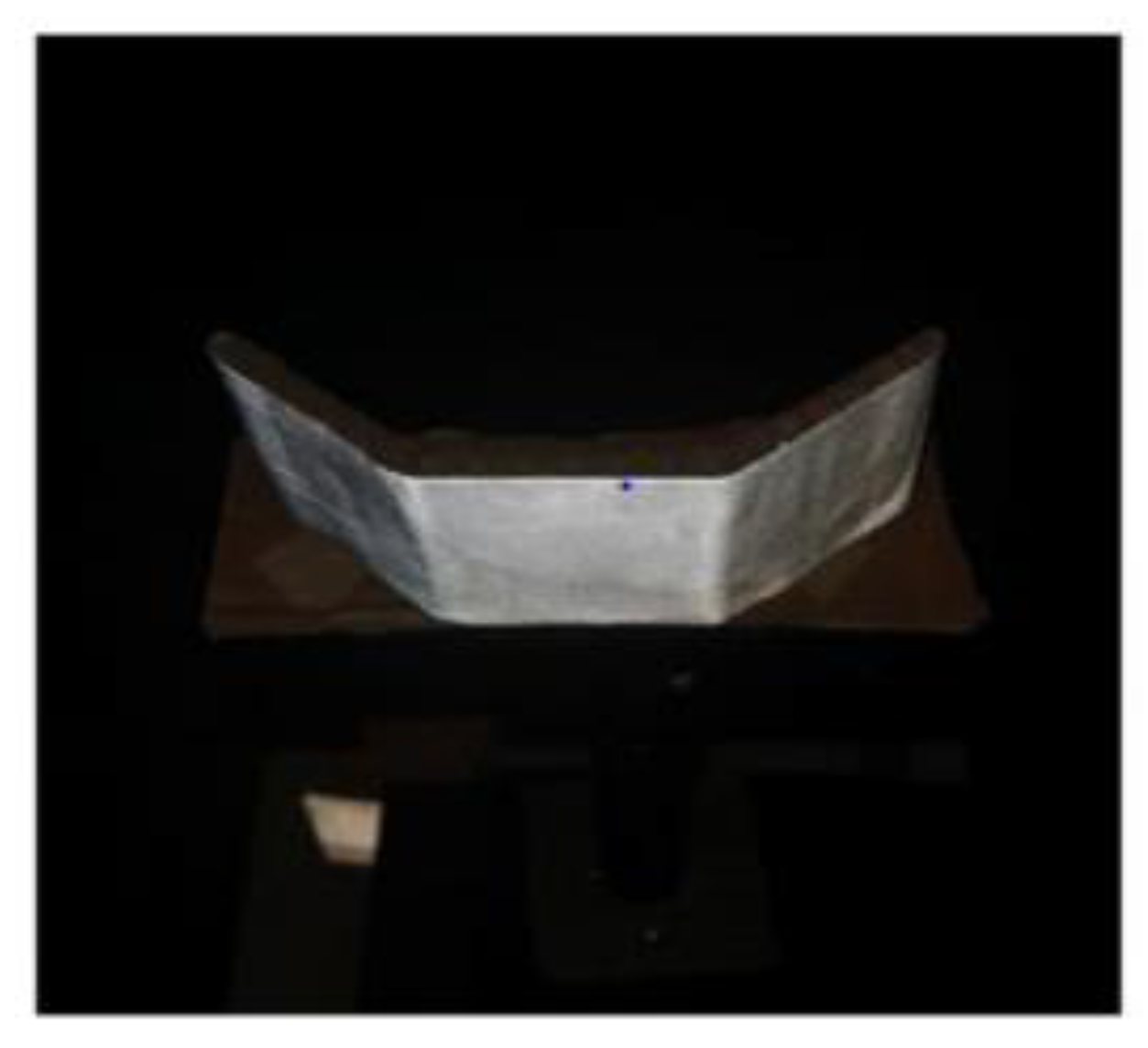
After meliorating the optical system in the laser transmitter and using a more advanced module, the far-field experiment is performed on the same detection target as shown in
Figure 5. After preprocessing the projection data,
Figure 10 shows the converted projection data of the far-field experiment. It is obvious that the quality of the projection data is significantly improved in that the echo data hardly fluctuate and their continuity is maintained well.
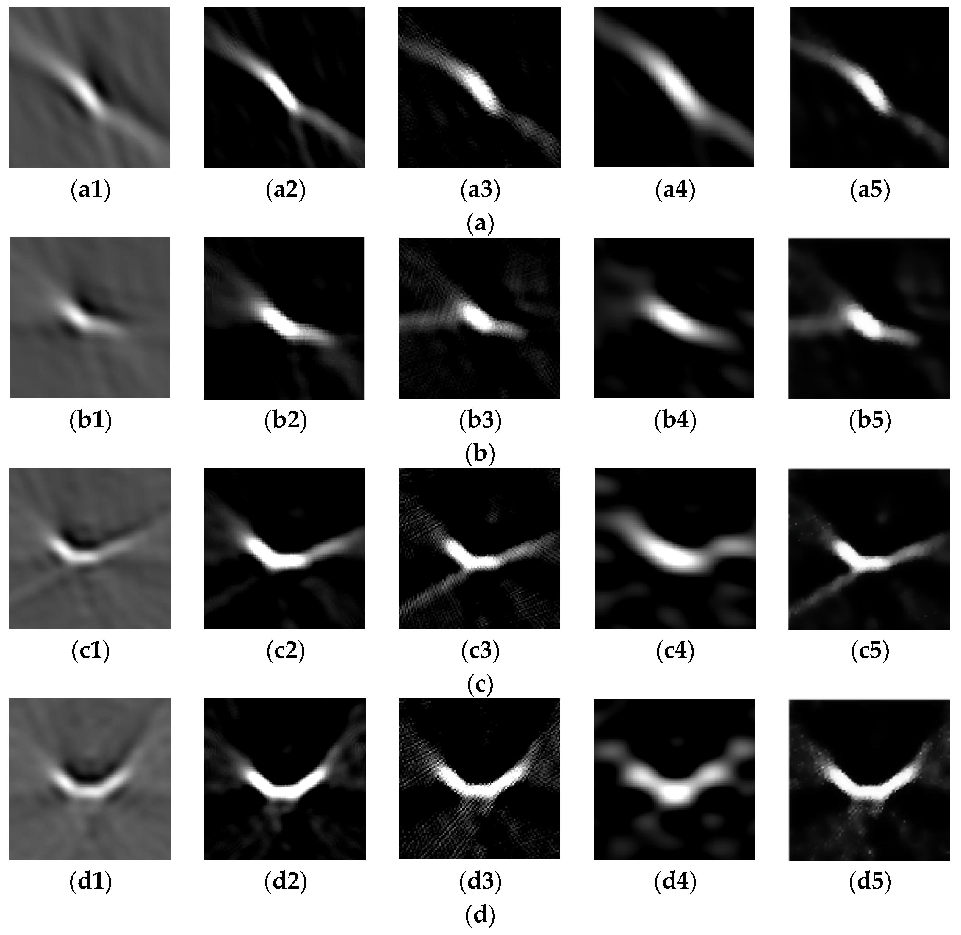
Similarly, for the projection data in the improved far-field experiment, the proposed imaging reconstruction algorithm is performed compared to iRadon, FBP, and ART with the complete view of projections and uniformly sampled projections in 5°, 10°, and 20° viewing intervals. The results are shown in
Figure 11.
As shown in
Figure 11, the reconstruction result is significantly optimized and the contour of the detection target is well embodied, which indicates that the new optical system has a great impact on the experiment. From the images in
Figure 11a, the included angle between each two squares can be clearly seen, overmatching the imaging results of the near-field experiment. However, it is also obvious that there are more artifacts in this experiment due to the influence of interference in the long distance.
The reconstruction effect of different algorithms resembles the result in the near-field experiment. The proposed TV sparse reconstruction with the ART algorithm shows a better effect under the circumstance of both complete view sampling and sparse sampling, which further proves the high precision of the algorithm.
Table 4 analyzes the IE, NRSNR, and Var of four approaches in far-field experiments. It can be clearly seen that the IE, NRSNR, and Var of the proposed method are still better than that of FBP, ART, and OMP. Take the results in 20° intervals as an example; the IE, NRSNR, and Var of the proposed method are 9.6316, 4.7132, and 0.0503, respectively, improved by about 160%, 50%, and 25% compared to that of other approaches. As a result, the effectiveness of the proposed TV sparse reconstruction with the ART algorithm in sparse views is again verified by the far-field experiment.
Figure 12 shows the second far-field experimental imaging results and then the same conclusion can be drawn as near-field experiments. In
Figure 12a,b, it can be clearly seen that the proposed method reconstructs the contour of the target well and performs better in denoising than the FBP and ART algorithms. In
Figure 12c, the reconstruction effect of random sampling is not ideal, but the proposed method generally restores the contour of the target, which proves to be effective in random sampling as well. As shown in
Table 5, the proposed method is still the best among the four algorithms, whether the projection data are added with noise or non-uniformly sampled, which proves the reliability of the proposed method once again. Furthermore, the NRSNR of the reconstructed image using the proposed method is also the highest, proving that the TV sparse reconstruction method possesses the character of working well when dealing with noise.
Finally, the proposed algorithm is tested under 0–60°, 90°, 120°, and 150° views of projections with new far-field data. When the viewing angle is less than 120° as in
Figure 13a,b, it is still hard to recognize the contour of the image. However, in this experiment, the image can be reconstructed well under the 150° view of projections as shown in
Figure 13c, which is superior to the near-field results. Further,
Figure 13(c5) shows that the quality of the reconstructed image using proposed algorithm in 150° view of projections can reach the same level as in complete angles. Correspondingly,
Table 6 analyzes the similarity between
Figure 13a–d and
Figure 11a in the form of CC. Furthermore, the superiority of the LRT TV-ART method is obvious according to the quantitative comparison in
Table 6.


 ,
, 


