Article

Advantages of Nonlinear Intensity Components for Contrast-Based Multispectral Pansharpening

1
Department of Information Engineering, University of Florence, 50139 Florence, Italy
2
Department of Information Engineering and Mathematics, University of Siena, 53100 Siena, Italy
3
CNR-IMAA, Consiglio Nazionale delle Ricerche, Contrada S. Loja snc, Tito Scalo, 85050 Potenza, Italy
4
CommSensLab, Department of Signal Theory and Communications, Universitat Politecnica de Catalunya, 08034 Barcelona, Spain
*
Author to whom correspondence should be addressed.
Remote Sens. 2022, 14(14), 3301; https://doi.org/10.3390/rs14143301
Submission received: 1 June 2022 / Revised: 2 July 2022 / Accepted: 4 July 2022 / Published: 8 July 2022

Abstract

:
In this study, we investigate whether a nonlinear intensity component can be beneficial for multispectral (MS) pansharpening based on component-substitution (CS). In classical CS methods, the intensity component is a linear combination of the spectral components and lies on a hyperplane in the vector space that contains the MS pixel values. Starting from the hyperspherical color space (HCS) fusion technique, we devise a novel method, in which the intensity component lies on a hyper-ellipsoidal surface instead of on a hyperspherical surface. The proposed method is insensitive to the format of the data, either floating-point spectral radiance values or fixed-point packed digital numbers (DNs), thanks to the use of a multivariate linear regression between the squares of the interpolated MS bands and the squared lowpass filtered Pan. The regression of squared MS, instead of the Euclidean radius used by HCS, makes the intensity component no longer lie on a hypersphere in the vector space of the MS samples, but on a hyperellipsoid. Furthermore, before the fusion is accomplished, the interpolated MS bands are corrected for atmospheric haze, in order to build a multiplicative injection model with approximately de-hazed components. Experiments on GeoEye-1 and WorldView-3 images show consistent advantages over the baseline HCS and a performance slightly superior to those of some of the most advanced methods.

1. Introduction

The availability of image data with spectral diversity (visible, near infrared, short wave infrared, thermal infrared, X- and C-band microwaves with related polarizations) and complementary spectral-spatial resolution, together with the peculiar characteristics of each image set, have fostered the development of fusion techniques specifically tailored to remotely sensed images of the Earth. Fusion aims at producing an extra value with respect to those separately available from the individual datasets. Though the results of fusion are more often analyzed by human experts to solve specific tasks (detection of landslides, flooded and burned areas, just to mention a few examples), partially supervised and also fully automated systems, most notably thematic classifiers, have started benefiting from fused images instead of separate datasets.
Extensive research on remote sensing image fusion for Earth observation has been carried out over the last decade, and a remarkable number of algorithms have been developed [1]. Image fusion techniques can be classified according to different criteria. One of the most common ways to differentiate fusion algorithms is based on sensor homogeneity. The term homogeneous image fusion refers to the case in which the images to be merged are produced by sensors exploiting the same imaging mechanism. This category is also called unimodal image fusion. In remote sensing for Earth observation, the fusion of panchromatic and multispectral (MS) images, also known as pansharpening, is a typical example of homogeneous image fusion. The images subject to fusion are the outcome of measurements of the reflected solar radiation of the scene, even though they are referred to different wavelengths and are characterized by different information contents, also in terms of spatial resolution. On the other hand, the fusion of heterogeneous data, or multimodal image fusion, is referred to those cases in which the data to be merged come from sensors not sharing the same imaging mechanism.
An additional way to discriminate among fusion techniques is based on the content level subject to fusion, i.e., pixel level, feature level, and decision level [1]. Pixel level image fusion directly combines the pixels of the involved images in order to produce a new image, whereas feature level fusion aims to combine specific features or descriptors extracted from the images to be merged. The extraction of the features can be performed either simultaneously on all the images or separately on each image. As an example, for the fusion of optical and Synthetic Aperture Radar (SAR) images [2], a direct merge of the two datasets is not recommended, to prevent contamination of the fusion product with the low signal-to-noise ratio (SNR) of SAR data. In this case, features extracted from the SAR image, either [3] for texture and spatial heterogeneity or [4] for temporal coherence of the scene derived from geocoded multilooked products, can be transplanted into the optical image, thereby alleviating the stringent requirement of co-registration between the two datasets typical of pixel-level fusion. Decision level fusion is the combination of the classification results achieved either from each dataset separately or from multiple algorithms on the same dataset. In this case, the fusion output is a classification map [5].
Among pixel-based remote-sensing image-fusion techniques, panchromatic (Pan) sharpening, or pansharpening, of multispectral (MS) images is receiving ever increasing attention [1,6]. Pansharpening takes advantage of the complementary characteristics of the spatial and spectral resolutions of MS and Pan data, originated by physical constraints on the SNR of broad and narrow bands [7]. The goal is the synthesis of a unique product that exhibits as many spectral bands as the original MS image, each with same spatial resolution as the Pan image.
After the MS bands have been interpolated and co-registered to the Pan image [8], spatial details are extracted from Pan and added to the MS bands according to a predefined injection model. The detail extraction step may follow the spectral approach, originally known as component substitution (CS), or the spatial approach, which may rely on multiresolution analysis (MRA), either separable or not [9]. In the spectral approach, the detail is the difference between the sharp Pan image and a smooth intensity component generated as a combination of the interpolated MS bands. In the spatial approach, the detail is the difference between the original Pan image and its version smoothed by a proper lowpass filter, retaining the same spatial frequency content of the MS bands. The dual classes of spectral and spatial methods exhibit complementary features in terms of tolerance to spatial and spectral impairments, respectively [10,11].
The Pan image is preliminarily histogram-matched, that is, radiometrically transformed by a constant gain and offset, in such a way that its lowpass version exhibits mean and variance equal to those of the component that shall be replaced [12]. The injection model rules the combination of the lowpass MS image with the spatial detail of Pan. Such a model is stated between each of the resampled MS bands and a lowpass version of the Pan image having the same spatial frequency content as the MS bands; a contextual adaptivity is generally beneficial [13]. The multiplicative, or contrast-based, injection model with haze correction [14,15] the key to improving the fusion performance by exploiting the imaging mechanism through atmosphere [16]. The injection model, which can rely on the most disparate criteria [17], is crucial for multimodal fusion, where the enhancing and enhanced datasets are produced by different physical imaging mechanisms, such as thermal sharpening [18]. The basic classification of CS and MRA has been progressively upgraded by considering several other methods that have been recently developed [6], such as those based on Bayesian inference [19], total variation (TV) regularization [20] and sparse representations [21]. More recently, machine learning paradigms have been introduced: since the pioneering study on pansharpening based on convolutional neural networks (CNN) [22], up to extremely sophisticated architectures, such as generative adversarial networks (GAN) [23]. It is noteworthy that, at least for methods based on learning concepts, histogram matching and detail-injection modeling are learned from the training data and implicitly performed by the network, without any control from the user. GAN architectures, however, are able to control one another, and thus, they are invaluable, e.g., for multimodal fusion [24].
This work deals with the use of nonlinear intensity components in spectral MS pansharpening methods. In fact, while CS methods, whose intensity components are linear combinations of the input bands, have been extensively investigated [1], nonlinear intensities have been seldom considered in the literature [25,26,27]. The hyperspherical color space (HCS) fusion technique [25] is perhaps the most widely known example. Analogously to the linear case, we propose a multivariate linear regression between the interpolated MS bands and the lowpass-filtered Pan. This time, however, the MS and Pan values are squared, before the regression is calculated. Hence, the intensity component no longer lies on a hyperplane in the vector space of the MS samples, as for the linear case, but on a hyper-ellipsoid. The proposed nonlinear intensity component is used in conjunction with the multiplicative injection model. Hence, the de-hazing procedure is extended to the nonlinear intensity.
In an experimental setup, GeoEye-1 and WorldView-3 data in spectral radiance format are pansharpened by several state-of-the-art and up-to-date methods, whose implementations are available in the Pansharpening Toolbox, originally conceived in [28]. The proposed method outperforms all the benchmarks on both the datasets, for all quality indexes at reduced resolution; in particular, its counterpart with linear intensity, referred to as Brovey transform with haze correction (BT-H) [15].
The remainder of this article is organized as follows. Section 2 provides the essential basics of pansharpening. Section 3 introduces the nonlinear intensity and describes the novel method. Section 4 is devoted to haze estimation of MS bands. Section 5 summarizes the adopted quality criteria and the related distortion indexes. Section 6 describes the two datasets and reports simulations and comparisons. Concluding remarks are presented in Section 7.

2. Basics of CS and Mra Pansharpening

Classical pansharpening methods can be divided into CS, MRA and hybrid methods. The unique difference between CS and MRA is the way to extract the Pan details, either by processing the stack of bands along the spectral direction or in the spatial domain. Hybrid methods, e.g., [29], are the cascade of CS and MRA, either CS followed by MRA or, more seldom, MRA followed by CS. In the former case, they are equivalent to MRA that inherits the injection model from the CS; in the latter case, they behave like CS, with the injection model borrowed from MRA [12]. Therefore, hybrid methods are not a third class with specific properties. The notation used in this paper will be firstly shown. Afterwards, a brief review of CS and MRA will follow.

2.1. Notation

The math notation used is detailed in the following. Vectors are indicated in bold lowercase (e.g., x ) with the ith element indicated as x i . 2-D and 3-D arrays are denoted in bold uppercase (e.g., X ). An MS image M = M k k = 1 , , N is a 3-D array composed of N spectral bands indexed by the subscript k. Accordingly, M k indicates the kth spectral band of M . The Pan image is a 2-D matrix indicated as P . The MS interpolated and pansharpened MS bands are denoted as M ˜ k and M ^ k , respectively. Unlike conventional matrix product and ratio, such operations are intended as product and ratio of terms of the same positions within the array.

2.2. CS

The class of CS, or spectral, methods is based on the projection of the MS image into another vector space, by assuming that the forward transformation splits the spatial structure and the spectral diversity into separate components.
Under the hypothesis of substitution of a single component that is a linear combination of the input bands, the fusion process can be obtained without the explicit calculation of the forward and backward transformations, but through a proper injection scheme, thereby leading to the fast implementation of CS methods, whose general formulation is [1]:
M ^ k = M ˜ k + G k · P ¯ ( I L ) I L , k = 1 , , N
in which k is the band index, G = [ G 1 , , G k , , G N ] the 3-D array of injection gains, which in principle may be different for each pixel each band, while the intensity, I L , is defined as
I L = i = 1 N w i · M ˜ i
in which the weight vector w = [ w 1 , , w i , , w N ] is the 1-D array of spectral weights, corresponding to the first row of the forward transformation matrix [1]. The term P ¯ ( I L ) is P histogram-matched to I L
P ¯ ( I L ) ( P μ P ) · σ I L σ P L + μ I L
in which μ and σ denote the mean and square root of variance, respectively, and P L is a lowpass version of P having the same spatial frequency content as I L [12].
The simplest CS fusion method is the Intensity–Hue–Saturation (IHS) [1], or better, its generalization to an arbitrary number of bands, GIHS, which allows a fast implementation, given by Equation (1) with unitary injection gains, G k = 1 .
The multiplicative or contrast-based injection model is a special case of Equation (1), in which space-varying injection gains, G , are defined such that
G k = M ˜ k I L , k = 1 , , N .
The resulting pansharpening method is described by
M ^ k = M ˜ k + M ˜ k I L · ( P ¯ ( I L ) I L ) = M ˜ k · P ¯ ( I L ) I L , k = 1 , , N
In Gram–Schmidt (GS) [30] spectral sharpening, the fusion process is described by Equation (1), where the injection gains are spatially uniform for each band, and thus denoted as g k k = 1 , , N . They are given by [12]:
g k = cov ( M ˜ k , I L ) var ( I L ) k = 1 , , N
in which cov X , Y indicates the covariance between X and Y , and var Y is the variance of Y . A multivariate linear regression has been exploited to model the relationship between the lowpass-filtered Pan, P L , and the interpolated MS bands [1,31].
P L = i = 1 N w ^ i · M ˜ i + b ^ + ϵ I ^ L + ϵ
in which I ^ L is the optimal intensity component and ϵ is the least squares (LS) space-varying residue. The set of space-constant optimal weights, { w ^ k } k = 1 , , N , and b ^ , is calculated as the minimum MSE (MMSE) solution of Equation (7). A figure of merit of the matching achieved by Equation (7) is given by the coefficient of determination (CD), namely R 2 , defined as
R 2 1 σ ϵ 2 σ P L 2
in which σ ϵ 2 and σ P L 2 denote the variance of the (zero-mean) LS residue, ϵ , and of the lowpass-filtered Pan image, respectively. Histogram-matching of Pan to the MMSE intensity component, I ^ L , should take into account that μ P = μ P L = μ I ^ L , from Equation (7). Thus, from the definition of CD in Equation (8)
P ¯ ( I ^ L ) = ( P μ P ) · R + μ P .
This brief review does not include a popular CS fusion method employing principal component analysis (PCA). The reason is that PCA is a particular case of the more general GS transformation, in which I L is equal to the maximum-variance first principal component, PC1, and the injection gains are those of GS (Equation (6)) [1].

2.3. MRA

The spatial approach relies on the injection of highpass spatial details of Pan into the resampled MS bands. The most general MRA-based fusion may be stated as:
M ^ k = M ˜ k + G k · P ¯ ( M ˜ k ) P ¯ L ( M ˜ k ) , k = 1 , , N .
in which the Pan image is preliminarily histogram-matched to the interpolated kth MS band [12]
P ¯ ( M ˜ k ) ( P μ P ) · σ M ˜ k σ P L + μ M ˜ k
and P ¯ L ( M ˜ k ) the lowpass-filtered version of P ¯ ( M ˜ k ) . It is noteworthy that according to either Equation (3) or Equation (11), histogram matching of P always implies the calculation of its lowpass version P L .
According to Equation (10) the different approaches and methods belonging to this class are uniquely characterized by the lowpass filter employed for obtaining the image P L , by the presence or absence of a decimator/interpolator pair [32] and by the set of space-varying injection gains, either spatially uniform, g k k = 1 , , N or space-varying, G k k = 1 , , N .
The contrast-based version of MRA pansharpening is
M ^ k = M ˜ k + M ˜ k P ¯ L ( M ˜ k ) · P ¯ ( M ˜ k ) P ¯ L ( M ˜ k ) = M ˜ k · P ¯ ( M ˜ k ) P ¯ L ( M ˜ k ) , k = 1 , , N .
It is noteworthy that, unlike what happens for Equation (5), Equation (12) does not preserve the spectral angle of M ˜ k because the multiplicative sharpening term depends on k, through Equation (11).
Eventually, the projective injection gains derived from GS in Equation (6) can be extended to MRA fusion as
g k = cov ( M ˜ k , P L ) var ( P L ) k = 1 , , N
whose space varying-version G k , with statistics calculated locally on a sliding window, coupled with a pyramid MRA constitutes a popular pansharpening method known as GLP-CBD [1,28].
Eventually, we wish to remind that spatial methods are favored if the spatial lowpass filters are designed in order to match the shape of the modulation transfer function (MTF), which is the spatial response in the Fourier domain of the imaging instrument and determines the amount of spatial information conveyed by each spectral channel [33].

3. Pansharpening Based on Nonlinear Intensity Components

The critical review of the baseline HCS [25] is based on the subsequent study by Tu et al. [26], who highlighted the advantages and limitations of the HCS approach. The first idea was to use the HCS transformation as an alternative to the intensity-hue-saturation (IHS) transformation, which had been already generalized to an arbitrary number of bands [1,26], as GIHS. Unfortunately, IHS features a unitary detail-injection model, which is generally poorer than the projection model (GS) and the multiplicative model of Brovey transform (BT) [1,34]. Therefore, in the subsequent publication [26], a fast multiplicative version of HCS was proposed. Fast because it is no longer necessary to calculate the direct and inverse hyperspherical transforms, but only the radius, which is used as intensity component of BT.
The (fast) HCS fusion [26] is given by Equation (5), with the MMSE intensity I L replaced by the HCS intensity, I L HCS , the radius of the N-dimensional hypersphere:
I L HCS = i = 1 N M ˜ i 2 .
The original contribution of the present study is to generalize the multivariate regression of Equation (7) to the case of Euclidean distance, as in Equation (14). The result is a new nonlinear intensity component, given by the RMS weighted value of the interpolated MS bands:
I ^ L HECS = i = 1 N w ^ i M ˜ i 2 + b ^
in which the set of N spectral weights, w ^ k , and the bias b ^ are found as the LS solution of the linear regression between squared MS and squared lowpass-filtered Pan:
P L 2 = i = 1 N w ^ i · M ˜ i 2 + b ^ + ϵ I ^ L HECS 2 + ϵ .
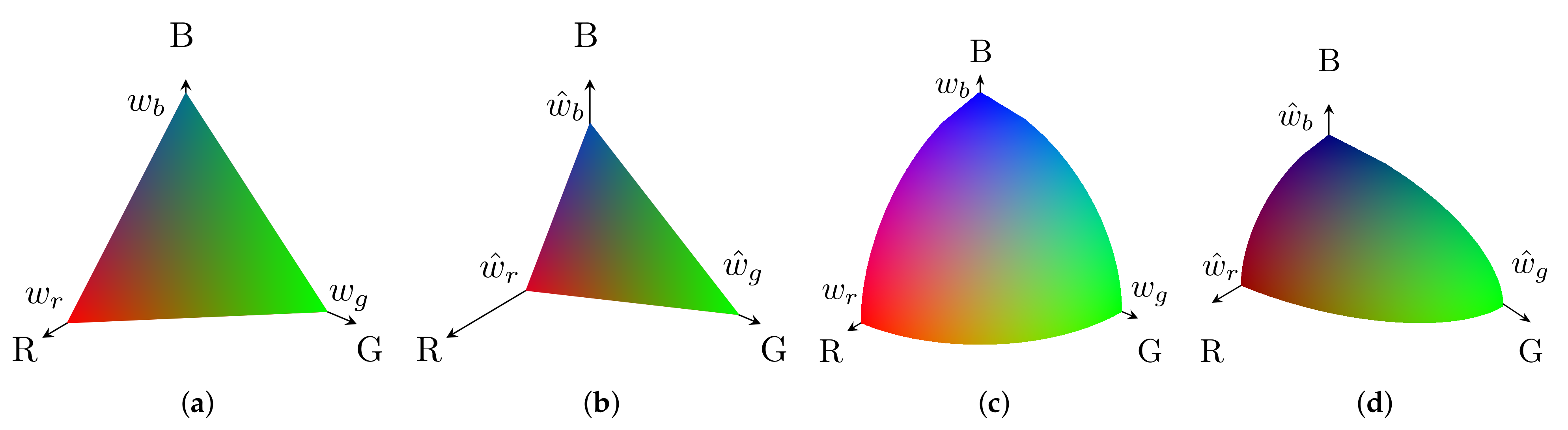
In the case of three bands, the color spaces of contrast-based fusion methods with linear and nonlinear intensities calculated with and without regression are displayed in Figure 1a–d. Notice that the linear intensity with prefixed equal weights of BT defines an equilateral triangle, as the intersection of a plane with the the first octant of the Euclidean space; the linear intensity with LS weights of BT-H [15] generally yields a scalene triangle. Conversely, as the color space of HCS is the section of a spherical surface lying in the first octant, the proposed method yields an ellipsoidal section. In fact, Equation (15) defines a hyper-ellipsoid, a generalization of the hypersphere in Figure 1c, when the weights may no longer be equal to one another; hence the name hyper-ellipsoidal color space (HECS) fusion.
The proposed scheme includes de-hazing, highly beneficial for fusion methods with a multiplicative detail-injection model [15,35]. Hence, the formulation of the proposed HECS pansharpening fusion is
M ^ k = M ˜ k L p k · P ¯ ( I ^ L HECS ) L p I ^ L HECS I ^ L HECS L p I ^ L HECS + L p ( k ) , k = 1 , , N
in which the path-radiance, or haze, of the synthetic intensity, L p ( I ^ L HECS ) , is given by the weighted RMS value of the individual path radiances, L p ( k ) , k = 1 , , N ,
L p P = L p P L = L p I ^ L HECS = i = 1 N w i ^ · L p 2 ( i ) + b ^ .
Equation (17) shows that the spectral pixel vector is translated by the haze vector before the multiplicative fusion is accomplished and the fused pixel vector is translated back by the same haze vector. 
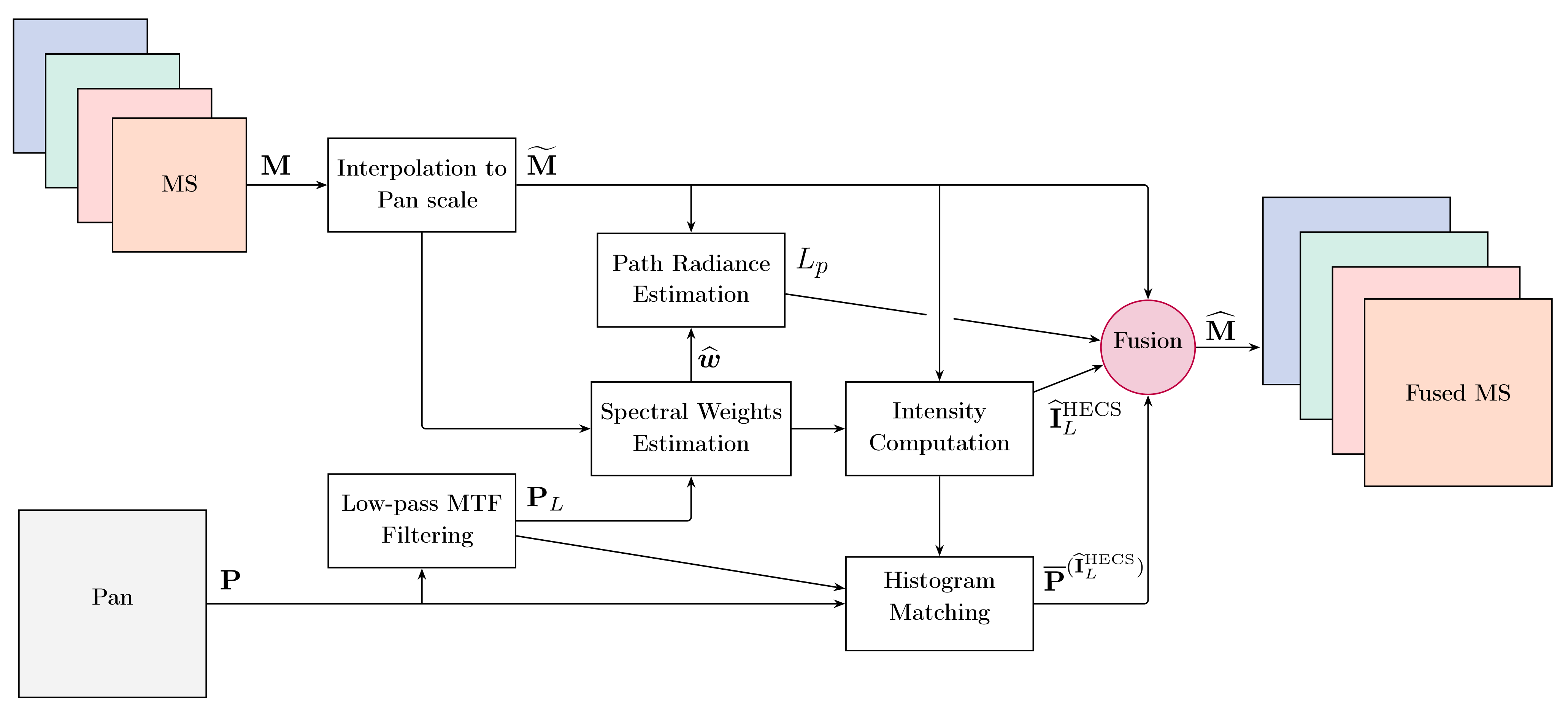
Figure 2 shows a flowchart describing the HECS fusion process. The estimation of the atmospheric path radiances of the individual MS bands will be tackled in the next section.

4. Haze Estimation

MS pansharpening, which produces a sharp MS image having the same format as the original MS image [12], generally does not require any kind of atmospheric corrections, unless a multiplicative detail-injection model is adopted [15]. In this case, it was proven that the haze-corrected pansharpening is capable of thoroughly preserving the map of normalized differential vegetation index (NDVI) of the original MS data [35].

4.1. Definition of Haze

All the different atmospheric constituents, as natural or anthropogenic aerosols that also have other important effects on population [36] and climate changes [37], gases (e.g., nitrogen, oxygen), and hydro-meteors (e.g., liquid and ice clouds, precipitation) scatter and absorb the incoming shortwave solar radiation. Haze is then the responsible for all the unwanted wavelength-dependent backscattered solar radiation by the previously described atmospheric components that does not go under an interaction with the Earth’s surface. Haze term correction requires path-radiance value estimation/calculation for the different spectral bands. Path-radiance estimation may follow image-based approaches or rely on radiative transfer models of the atmosphere and its constituents, as well as on knowledge of acquisition parameters, such as the actual Sun–Earth distance, solar zenith angle and satellite platform observation angle.
Image-based atmospheric correction techniques [38] are a series of statistical methods based on some general assumptions and empirical criteria. The goal is estimating the atmospheric effects on acquisition without requiring acquisition parameters or making assumptions on atmospheric constituents. If the band offsets (metadata) in the file header are all identically zero, image-based methods are also directly applicable without a preliminary conversion. In this case, the path-radiance values estimated for each band will not be expressed in physical units, but as DNs. Conversion to spectral radiance units, typically [W · m−2 · sr−1 · μm−1] or [mW · cm−2 · sr−1 · μm−1] requires subsequent multiplication by the calibration gain metadata. If the offsets are nonzero, it is preferable to convert all pixel values to physical units before applying image-based methods.

4.2. Shadowed Pixel Assumption

In order to apply image-based methods to estimate the path-radiance values, let us make a series of assumptions: (i) the path radiance is uniform over the scene; (ii) the scene is large enough, in terms of number of pixels, and hence statistically consistent; (iii) the scene contains shadowed pixels where the direct solar irradiance is masked by some obstacle; (iv) the diffuse irradiance at the surface is an order of magnitude smaller with respect to the direct solar irradiance. Under those assumptions, the path radiance of the kth band will be equal to the minimum of spectral radiance attained over the kth band of the scene. In practice, instead of the minimum (0-percentile) the haze is taken equal to the 1-percentile of the histogram. This strategy is robust and permits us to deal with the small, but non-zero, diffuse irradiance and to the photon and thermal instrument noise appearing as fluctuations of the dark signal around its average, and to outliers originated by pattern-gain correction of the instrument. The spatial scale of representation is crucial: a full shadowed pixel at higher spatial resolution might not be anymore when mapped onto larger pixels. The path radiance arguably does not depend on the spatial scale. Scale invariance at 2 m and 8 m is attained considering percentile values between 0.5 and 1. Below 0.5, the invariance is weak while above 1, the invariance is almost perfect. Thus, the path radiance of the kth band, which is usually approximated by its minimum (0-percentile) over the scene [38,39], may be better approximated by any value between the 0.5-percentile and the 1-percentile.
If the scene does not contain at least one pure shadow pixel, i.e., snow-covered surfaces or desert environment, the above method may lead to serious estimation errors. A shortcoming would be assuming that at least one pixel in the scene has a reflectance close to zero [39]. This assumption is unlikely for all wavelengths, but may approximately hold for the blue (B) band, where the atmospheric Rayleigh scattering is ten times stronger with respect to the red band (R).

4.3. Haze Computation

So, once the path-radiance of the B channel, L p (B), is known, being estimated as a small percentile of the local histogram, the intercept of the scatterplot of G versus (B-–Lp(B)) is an estimate of the path radiance of the green (G) channel, Lp(G); analogously for the red (R) channel, Lp(R) may be estimated from the R-to-(G–Lp(G)) scatterplot. The scatterplot method holds for the visible bands [38]. For calculating the path radiance of NIR, which is practically uncorrelated with the visible bands in the presence of vegetation [40], the scatterplot method may fail, unless its calculation, either supervised or unsupervised, e.g., NDVI-enforced, is performed on non-vegetated areas. Otherwise, a reasonable physical approximation is that the Lp(NIR) is set equal to zero.
Additionally, a modeling of the atmosphere is an option. In this case, the DNs must be preliminarily calibrated by means of the gains and offsets metadata. Radiative transfer modeling requires acquisition year, month, day, local time, longitude, latitude, and possibly type of landscape for setting aerosols (advected [41] or local) both in the boundary layer or upper troposphere. The content of water vapor may be inferred from estimation of the rain evaporation rate [42]. The Fu–Liou–Gu (FLG) model [43] directly yields values of path-radiance in predefined bands, roughly corresponding to those of MS scanners, such as Landsat 8 OLI. With small adjustments to fit the R and NIR bands of GeoEye-1, it was recently found [35] that the modeled path radiance is well approximated by 95% of the 1-percentile of B, 65% of the 1-percentile of G, 45% of the 1-percentile of R and 5% of the 1-percentile of NIR.
An exhaustive search at steps of one DN was performed in [15]. The optimal values of path-radiances are those that optimize fusion scores, on average, at the degraded spatial scale, i.e., when the ground truth is available as reference. With FLG-modeled path radiances and model-enforced image-based path-radiances, the performance is about 0.1% lower than that achieved with the exhaustive search. Therefore, the accuracy of path radiance estimation is not crucial, at least for clear atmospheres. Interestingly, the fusion performance plots vs. corrected path-radiance values exhibit a maximum that is peaked for under-corrected haze and much flatter for over-corrected haze. This fact entails the use of band minima as estimated haze values, that is, L P k = min M k , k = 1 , , N .
Trivially, the haze term is zero for data in surface reflectance format, whenever they are available. The surface reflectance is a level-two (L2) product and is distributed for global-coverage systems (OLI, Sentinel-2), only where an instrument network is available for atmospheric measurements [44], usually carried out by means of lidar instruments [45,46].

5. Quality Assessment

Quality evaluation of image fusion products has been, and still is, the object of extensive research. The problem is complicated by the fact that it may not be easy to formalize what “quality” means in the fusion process. In this regard, a protocol of assessment should have very clear objectives and possibly require a reference on which the comparison relies. Image fusion assessment is traditionally performed in two ways: (1) by means of a human visual inspection by a panel of investigators; and (2) through mathematical functions capable of objectively measuring or inferring the similarity of the fusion product to a reference target, which is always unavailable and often also undefined. Whereas the former is based on subjective human evaluations that can be embodied by some statistical indexes, such as entropy, contrast, gradient, and so on [24], the objective evaluation involves stringent and quantitative measures that involve both original and fused images and are possibly consistent with human visual perception. In the fusion of medical images, it is crucial to preserve the diagnostic characteristics of the original images within the fused image; thus, it is necessary to evaluate the result of the fusion process using objective parameters.
In remote sensing image fusion, especially multispectral pansharpening applications, quality assessment is performed following Wald’s protocol [47], which substantially requires the fused image to satisfy three main properties:
-
Consistency: the fused image, once spatially degraded to the original resolution, should be as close as possible to the original image;
-
Synthesis: any low-resolution (LR) image fused by means of a high-resolution (HR) image should be as identical as possible to the ideal image that the corresponding sensor, if existent, would observe at the resolution of the HR image.
-
Vector synthesis: the set of multispectral images fused by means of the HR image should be as identical as possible to the set of ideal images that the corresponding sensor, if existent, would observe at the spatial resolution of the HR image.
The property of consistency is usually easier to assess since the original LR image can be used as a reference. Only the procedure of spatial degradation and the matching function are to be standardized. On the contrary, the synthesis property is harder to be verified, since a reference is required. A viable shortcoming stems from the assumption of scale-invariance of the scene, that is, quality measures do not vary with the resolution, at which the scene is imaged. This allows the quality to be measured at a resolution lower than the original one, for which the reference image is available.
More specifically, the process consists of spatially degrading both the enhancing and the enhanced datasets by a factor equal to the scale ratio between them and using the original LR image as reference. Obviously, such an assumption is not always valid, especially when the degradation process does not mimic the actual sensor acquisition process. In the case of multimodal image fusion, the applicability of the synthesis properties of the Wald’s protocol is questionable since a multimodal fusion method aims at producing images in which the features coming from different sensors should in principle be both present. If the imaging sensors exploit different physical mechanisms, e.g., reflectivity and emissivity in the case of fusion of optical and thermal data, the assumption that an “ideal” sensor producing the fused image could exist is unlikely, since such a sensor should be able to measure and integrate different physical phenomena at the same time.
In conclusion, notwithstanding achievements over years [48,49,50,51,52,53,54], quality assessment of pansharpened images is still an open problem, being inherently ill-posed. A further source of uncertainty, which has been explicitly addressed very seldom [55,56], is that the measured quality may also depend on the data format.

5.1. Reduced-Resolution Assessment

The quality check often entails the shortcoming of performing fusion with both MS and Pan datasets degraded at spatial resolutions lower than those of the originals, in order to use non-degraded MS originals as quality references [57]. Here, some popular statistical similarity/dissimilarity indexes used in this study will be briefly reviewed.

5.1.1. SAM

The spectral angle mapper (SAM) was originally introduced for the discrimination of materials starting from their reflectance spectra [58]. Given two spectral vectors, v and v ^ , both having N components, in which v = { v 1 , v 2 , , v N } is the reference spectral pixel vector and v ^ = { v ^ 1 , v ^ 2 , , v ^ N } is the test spectral pixel vector, SAM denotes the absolute value of the spectral angle between the two vectors:
SAM ( v , v ^ ) arccos < v , v ^ > | | v | | 2 · | | v ^ | | 2 .
SAM is usually expressed in degrees and is equal to zero if the test vector is spectrally identical to the reference vector, i.e., the two vectors are parallel and may differ only by their moduli. A global spectral dissimilarity, or distortion, index is obtained by averaging Equation (19) over the scene.

5.1.2. ERGAS

ERGAS, the French acronym for relative dimensionless global error in synthesis [59], is the cumulative normalized root mean square error (NRMSE) between test and reference band, multiplied by the Pan-to-MS scale ratio and expressed in percentage:
ERGAS 100 d h d l 1 N k = 1 N RMSE ( k ) μ ( k ) 2
where d h / d l is the ratio between pixel sizes of Pan and MS, e.g., 1/4, μ ( k ) is the mean (average) of the kth band of the reference and N is the number of bands. Low values of ERGAS indicate high similarity between fused and reference MS data.

5.1.3. Multivariate UIQI

Q2n is the multiband extension of the universal image quality index (UIQI) [60] and was introduced for quality assessment of pansharpened MS images [61]. Each pixel of an image with N spectral bands is accommodated into a hypercomplex (HC) number with one real part and N 1 imaginary parts.
Let z = z ( m , n ) and z ^ = z ^ ( m , n ) denote the HC representation of the reference and test spectral vectors at pixel ( m , n ) . Analogously to UIQI, namely, Q20=Q, Q2n may be written as product of three terms:
Q 2 n = | σ z z ^ | σ z σ z ^ · 2 σ z σ z ^ σ z 2 + σ z ^ 2 · 2 | z ¯ | | z ^ ¯ | | z ¯ | 2 + | z ^ ¯ | 2
the first of which is the modulus of the HC correlation coefficient (HCCC) between z and z ^ . The second and third terms, respectively, measure contrast changes and mean bias on all bands simultaneously. Statistics are calculated on square blocks, typically, 32 × 32, and Q2n is averaged over the blocks of the whole image to yield the global score index. Q2n takes values in [0, 1] and is equal to 1 iff z = z ^ for all pixels.

5.2. Full-Resolution Assessment

Quality can be evaluated at the original panchromatic scale, according to a full resolution (FR) approach [62]. In this case, the spectral and spatial distortions are separately evaluated starting from the fused image and either the original low-resolution MS bands or the high-resolution panchromatic image, as firstly proposed by Zhu et al. [63].

5.2.1. QNR

A widely adopted FR assessment is based on the quality with no reference (QNR) protocol [51] and the related distortion indexes. QNR combines into a unique overall quality index a spectral distortion measure between the original and pansharpened MS bands and a spatial distortion measure between each MS band and PAN. The QNR protocol is based on the following assumptions:
  • The fusion process should not change the intra-relationships between couples of MS bands; in other words, any intra-relationship changes between couples of MS bands across resolution scales are considered as indicators of spectral distortions;
  • The fusion process should not change the inter-relationships between each MS band and the Pan image; in other words, any inter-relationship changes between each MS band and the Pan across resolution scales are modeled as spatial distortions.
The QNR protocol employs the UIQI as a similarity measure and the absolute difference as the change operator. The spectral distortion index, D λ , is obtained by computing two sets of UIQI values, each between couples of MS bands. Afterward, their absolute difference is taken and averaged:
D λ = 1 N ( N 1 ) l = 1 N r = 1 r l N | Q ( M ˜ l , M ˜ r ) Q ( M ^ l , M ^ r ) | .
The spatial distortion index, D s , is computed by means of the average absolute UIQI band by band difference, between MS and Pan, both at FR and at the original MS resolution:
D s = 1 N i = 1 N | Q ( M ˜ i , P L ) Q ( M ^ i , P ) | .
Finally, a unique quality index is obtained combining the complement of spatial and spectral distortion indexes:
QNR = ( 1 D λ ) α · ( 1 D s ) β .
The exponents α and β rule the balance of the spectral and spatial quality components. They can be normalized in such a way that α + β = 1 . In this case, if α = β = 0.5 , Equation (24) yields the geometric mean of the spectral and spatial qualities, though normalization of exponents compresses the variability of the cumulative index. Typical values for the exponents are α = β = 1 .

5.2.2. Khan’s QNR

A totally different approach was later proposed by Khan et al. [52]. Analogously to QNR, Khan’s QNR (KQNR) defines and combines spectral and spatial consistency factors. The innovations introduced by the KQNR protocol is to make use of the consistency property of Wald’s protocol to calculate the spectral consistency of the pansharpened product. Since the consistency property evaluation requires a spatial degradation stage, including a decimation operation, the KQNR protocol proposes to use MTF-matched filters to perform the spatial degradation of the fused MS bands. Thus, the spectral distortion index, D λ ( K ) , is computed according to the following procedure:
  • Each fused MS band is spatially degraded (filtered and decimated) with its specific MTF-matched filter;
  • The Q 2 n index between the set of spatially degraded fused MS images and the original MS dataset is computed;
  • The one’s complement is taken to obtain a distortion measure:
D λ ( K ) = 1 Q 2 n ( M ^ L , M ) .
The spatial consistency of Khan’s protocol is given by the average change in interscale similarities between highpass components of each fused band and Pan:
D s ( K ) 1 N k = 1 N | Q ( M ^ k H , P H ) Q ( M k H , ( P L ) H ) | .
Again, a cumulative quality index is obtained combining the complement of spatial and spectral distortion indexes:
QNR = ( 1 D λ ( K ) ) α · ( 1 D s ( K ) ) β
with typical values for the exponents α = β = 1 .
It is noteworthy that, unlike what happened with QNR, the KQNR protocol states the the spectral and spatial consistencies are calculated on the lowpass and highpass spatial-frequency channels of the fused images; in the former case with a comparison with the original MS; in the latter case with a comparison with the highpass components of the original Pan and of the spatially degraded Pan.

5.2.3. Hybrid QNR

The hybrid QNR (HQNR) has been presented in [53] as the combination of the spectral distortion index of KQNR in Equation (25) with the spatial distortion index of QNR in Equation (23).
Analogously to QNR and KQNR, a unique quality index is obtained combining the one’s complements of the spectral and spatial distortions:
HQNR = 1 D λ ( K ) α · 1 D s β .
For the sake of completeness, we could consider the dual of HQNR (DQNR), in which the spectral distortion in Equation (22) is coupled with the spatial distortion in Equation (26), defined as:
DQNR = 1 D λ α · 1 D s ( K ) β .

6. Experimental Results and Discussion

6.1. Data Sets

Two test images, acquired by two different platforms, GeoEye-1 and WorldView-3, have been used in the simulations. In this section, besides describing the two datasets, which belong to the reference pansharpening dataset, namely PAirMax, described in [64], we present an analysis of the solution of the multivariate regressions (Equations (7) and (16)) for the two datasets.

6.1.1. Trenton Dataset

The GeoEye-1 image has been acquired over the area of Trenton NJ, USA, on 27 September 2019. The on-orbit limit sampling interval at nadir (half the system’s resolution) is 1.64 m for MS and 0.41 m for Pan. The spatial sampling interval (SSI) of the resampled geocoded product is 2 m for MS and 0.5 m for Pan, resulting in a scale ratio equal to four. The MS image features four spectral bands: blue (B), green (G), red (R) and near infra-red (NIR). The image size is 512 × 512 pixels for MS and 2048 × 2048 for Pan. The radiometric resolution of the DN format is 11 bits; the conversion coefficients to the SR format, extracted from the metadata, are reported in Table 1. It is noteworthy that the offsets are all equal to zero.

6.1.2. Munich Dataset

The WorldView-3 image, acquired on 10 January 2020, portrays the city of Munich, Germany, and surrounding agricultural fields and forested areas. The on-orbit limit sampling interval at nadir is 1.24 m for MS and 0.31 m for Pan. The SSI is 1.32 m for MS and 0.33 m for Pan; hence, the scale ratio is still four. The MS image comprises eight bands: coastal (C), B, G, yellow (Y), R, red edge (RE), NIR1 and NIR2. The covered area is 456,759 m2, corresponding to MS and Pan image sizes of 512 × 512 and 2048 × 2048 pixels, respectively. The fixed-point representation of the data employs 11 bits. Table 2 shows the corresponding radiometric calibration coefficients obtained from the metadata file. Moreover, in this case, the offsets are identically equal to zero.

6.2. Analysis of the LS Intensity Component

The LS solutions of the multivariate linear regression, both Equations (7) and (16), are now discussed for the two test datasets. Table 3 and Table 4 report the MMSE spectral weights of each band and the bias coefficients, if they are included, for both the datasets preliminarily converted to SR format. The regression of squares in Equation (16) produces spectral weights that are far different from the other case. However, it is equivalent to Equation (7) in terms of matching success, for Trenton; slightly less fitting for Munich, supposedly, because the bandwidth of Pan does not include the outermost MS bands of WorldView-3. In both regressions, Equations (7) and (16), the presence or absence of the bias term produces w ^ k s that are somewhat different, especially for Munich, but this has very limited impact on the degree of matching, measured by CD, which changes by 10 5 for Munich and even less for Trenton.

6.3. Simulations

Twelve pansharpening algorithms, including the plain interpolated MS image, without injection of details, denoted by EXP, have been selected from the Pansharpening Toolbox [6,28]. The list includes:
  • Brovey transfom (BT) [1,34];
  • Gram–Schmidt (GS) spectral sharpening [1,30];
  • Fast fusion with hyperspherical color space (HCS) [26];
  • Optimized BT with haze correction (BT-H) [15];
  • GS with adaptive intensity (GSA) [1,28];
  • The proposed method with hyper-ellipsoidal color space (HECS);
  • Fusion method with band-dependent spatial-details (BDSD) injection [65];
  • Additive wavelet luminance proportional with haze correction (AWLP-H) [31];
  • GLP with MTF filters and full-scale detail injection modeling (MTF-GLP-FS) [66];
  • Fusion based on sparse representation of spatial details (SR-D) [21];
  • Fusion based on total-variation (TV) optimization [20];
  • Advanced pansharpening with neural networks and fine tuning (A-PNN-FT) [22].
Table 5 reports the numerical results of the RR simulations performed on the two datasets. There is a significant increment in performance of HECS over its baseline HCS. Comparisons with BDSD, BT-H and AWLP-H reveal that the three haze-corrected methods are practically equivalent in performance. The performance of BT is noteworthy for Trenton, but average for Munich. In fact, the intensity component calculated as an average of the interpolated MS bands attains a high degree of matching with the lowpass-filtered Pan: CD equal to 0.9904, very similar to the CDs of BT-H and HECS in Table 3. The high CD and the small amount of vegetated areas, from which haze correction benefits, in the Trenton image, makes all contrast-based CS methods perform very similar to one another, regardless of their intrinsic structure, more or less developed. Overall, HECS outperforms all the other methods in all quality parameters on the Munich test site. On the Trenton image, the performance of A-PNN-FS in terms of SAM stands out.
The results of the fusion process at reduced resolution for each of the methods, are shown in Figure 3, for the datasets of Munich. HCS is visually sharp, but colors are somewhat distorted. The three haze-corrected methods, BT-H, AWLP-H and HECS look very similar to one another. BDSD is fine but the tree canopies are unrealistically textured. SR-D surprisingly exhibits striping artifacts in built-up areas.
Table 6 reports the numerical results of the FR simulations performed on the Trenton dataset. Such results are reported for the four main distortions, two spectral and two spatial, and for all the four possible combinations of a spectral and a spatial distortion, considered in Section 5.2. Apart from EXP, SR-D, TV and A-PNN-FT, which do not follow the strict classification of spectral and spatial methods, BT, GS, HCS, BT-H, GSA, HECS and BDSD are methods based on CS; AWLP-H and MTF-GLP-FS on MRA. In the ranking of methods provided by QNR, BDSD is the first method, TV the second best and HECS the third one. The raking provided by KQNR and HQNR is far different: HECS is at the sixth place for KQNR and even at the seventh for HQNR. Eventually, DQNR provides a totally different ranking, more similar to that of QNR, in which HECS is in first position, closely follows by AWLP-H. This puzzling behavior of the FR quality indexes has a twofold explanation: (i) the spatial distortion of QNR in Equation (23) was found to be very sensitive to the choice of the decimation filter of Pan [57], which is unknown in FR experiments; (ii) according to Khan’s protocol, all CS methods exhibit very high values of spectral distortion (Equation (25)) and the sole possible explanation [6,62] is that, due to the presence of hardly perceivable space-varying misaligments between interpolated MS and Pan, CS methods shift the fused MS towards Pan, thereby losing its consistency towards the original MS [8,67]. If we restrict the comparison of HECS to CS methods only, we will find that for all cumulative indexes containing the spectral distortion in Equation (25), namely KQNR and HQNR, HECS is the best among CS methods, though poorer than those methods that are not CS. We can conclude that in quantitative assessments carried out at FR, HECS confirms its superiority, though moderate, over benchmarks that represent the state-of-the art of MS pansharpening.
The results of the FR fusion process are shown in Figure 4, for the datasets of Trenton. GS, BT, HCS and GSA are very similar to one another: clean and geometrically fine, but with little distortion of color spots. BT-H and HECS are very similar: geometrically accurate, adequately textured (thanks to dehazing), with spectral brightness of color spots, slightly better for HECS (see colored cars). BDSD is finely textured, with bright color spots, but little realistic. AWLP-H and MTF-GLP-FS are rather fine, but less geometrically accurate than CS methods, presumably due to misalignment of datasets. SR-D is unrealistically over-textured. TV is accurate, but slightly little sharp. A-PNN-FT is generally fine, though the typical glitch effects of neural methods are visible. In conclusion, the visual evaluations substantially agree with the ranking of methods achieved by means of DQNR. The ranking of QNR is partially flawed. KQNR and HQNR exhibit little agreement with visual evaluations, because spectral consistency measurements are impaired by the imperfect alignment.

6.4. Discussion

After a careful analysis of RR and FR results, both numerical indexes and true-color icons, a series of considerations can be made. Among methods featuring the multiplicative detail injection model, those performing haze correction (BT-H, HECS and AWLP-H) provide superior performance in the presence of vegetated areas. On the urban landscape of Trenton, the difference in performance, as measured in Table 5, among BT, BTH-H, HCS, HECS and AWLP-H is small.
The regression is crucial for the calculation of the injected detail, not for the injection model. In this sense, BT-H is slightly better than AWLP-H, where the two methods have exactly the same injection model and the same haze correction.
The question that arises is: why the proposed HECS is slightly better than BT-H, its counterpart employing a linear intensity (see Figure 1b,d). In Equation (17), the narrow-band haze terms are the same as for BT-H, the definition of the intensity component and the broadband haze terms of Equation (18) are different from those of BT-H, but identical at numerator and denominator of the ratio in Equation (17). If the broadband haze terms of HECS and BT-H are swapped, both methods slightly lose performance. Histogram matching of Pan to the intensity component is standard, as in Equation (3).
A reasonable explanation is that the regression of quadratic values in Equation (17) is such that the resulting LS intensity component better matches the lowpass-filtered Pan than the intensity achieved through a linear regression. With reference to Table 3 and Table 4, the CDs of the quadratic cases are slightly lower than those of the corresponding linear cases, but in the former case CD, measures the extent to which the squared intensity matches the squared lowpass-filtered Pan, in the latter case the extent to which the intensity matches the lowpass-filtered Pan. HECS takes the square root of the LS squared intensity, whose CD would be approximately equal to the square root of the CD of the regressions of squares, and hence greater for the intensity of HECS. Approximately, because the exact CD depends on the distribution of the random variables involved in the regression. With reference to Figure 1b,d, we can conclude that HECS is slightly better than BT-H, because the intensity component lying on a hyper-ellipsoid matches the lowpass-filtered Pan better than the intensity component lying on a hyperplane.
Eventually, the computational cost of all methods employing multivariate regressions (GSA, BT-H, AWLP-H and HECS) is practically identical, because all methods exploit fast algorithms [1,6] in which only the intensity component is calculated and the inverse transformation, also in the nonlinear case of HECS, does not require inversion, thanks to the multiplicative injection gains [26]. Out of the methods compared, SR-D [21] is the slowest, TV [20] intermediate, and all the others are fast, if we do not consider the training time of A-PNN-FT [22].

7. Concluding Remarks

In this paper, we have presented an enhanced version of a popular CS pansharpening method, the HCS fusion technique. The proposed method is insensitive to the format of the data [56], either spectral radiance values or packed digital numbers (DNs), thanks to the use of a multivariate linear regression between the squared interpolated MS bands and the squared lowpass-filtered Pan, in order to find out the MMSE intensity component, which is no longer a linear combination of the interpolated bands. The regression of squares, instead of the Euclidean radius of HCS, makes the color space hyper-ellipsoidal instead of hyperspherical. Furthermore, before fusion is performed, the interpolated MS bands are corrected for the atmospheric path radiance, in order to build a multiplicative injection model with approximately de-hazed components, thus benefiting from the haze correction, crucial for methods exploiting multiplicative detail-injection models [14,15,31,35].
Experiments on true GeoEye-1 and WorldView-3 data show significant advantages over the baseline HCS and its improvements achieved over time. A performance superior to some of the most advanced methods in the literature, including some new-generation methods based on variational optimization, either model based [20,21] or not [22], is achieved. The proposed fusion based on a hyper-ellipsoidal color space (HECS) retains the computational benefits of HCS and the robustness to local misregistration typical of all CS methods.

Author Contributions

Conceptualization and methodology: A.A., L.A., A.G. and S.L.; validation and software: A.A. and A.G.; data curation: A.G.; writing: L.A. and S.L. All authors have read and agreed to the published version of the manuscript.

Funding

This research received no external funding.

Data Availability Statement

Image data supporting the reported results are part of the dataset collection freely distributed by Maxar at https://resources.maxar.com/product-samples/pansharpening-benchmark-dataset (accessed on 31 May 2022).

Acknowledgments

The authors wish to give full credit and recognition to the invaluable support of their former coauthor, Bruno Aiazzi, prematurely passed away in December 2021, with whom the present study was originally conceived.

Conflicts of Interest

The authors declare no conflict of interest.

References

  1. Alparone, L.; Aiazzi, B.; Baronti, S.; Garzelli, A. Remote Sensing Image Fusion; CRC Press: Boca Raton, FL, USA, 2015. [Google Scholar]
  2. Aiazzi, B.; Alparone, L.; Arienzo, A.; Garzelli, A.; Zoppetti, C. Monitoring of changes in vegetation status through integration of time series of hyper-sharpened Sentinel-2 red-edge bands and information-theoretic textural features of Sentinel-1 SAR backscatter. In Proceedings of the Image and Signal Processing for Remote Sensing XXV, Strasbourg, France, 9–11 September 2019; Bruzzone, L., Ed.; SPIE: Bellingham, WA, USA, 2019; Volume 11155, pp. 111550Z-1–111550Z-12. [Google Scholar]
  3. Aiazzi, B.; Alparone, L.; Baronti, S. Information-theoretic heterogeneity measurement for SAR imagery. IEEE Trans. Geosci. Remote Sens. 2005, 43, 619–624. [Google Scholar] [CrossRef]
  4. Aiazzi, B.; Alparone, L.; Baronti, S.; Garzelli, A. Coherence estimation from multilook incoherent SAR imagery. IEEE Trans. Geosci. Remote Sens. 2003, 41, 2531–2539. [Google Scholar] [CrossRef]
  5. D’Elia, C.; Ruscino, S.; Abbate, M.; Aiazzi, B.; Baronti, S.; Alparone, L. SAR image classification through information-theoretic textural features, MRF segmentation, and object-oriented learning vector quantization. IEEE J. Sel. Top. Appl. Earth Observ. Remote Sens. 2014, 7, 1116–1126. [Google Scholar] [CrossRef]
  6. Vivone, G.; Dalla Mura, M.; Garzelli, A.; Restaino, R.; Scarpa, G.; Ulfarsson, M.; Alparone, L.; Chanussot, J. A new benchmark based on recent advances in multispectral pansharpening: Revisiting pansharpening with classical and emerging pansharpening methods. IEEE Geosci. Remote Sens. Mag. 2021, 9, 53–81. [Google Scholar] [CrossRef]
  7. Thomas, C.; Ranchin, T.; Wald, L.; Chanussot, J. Synthesis of multispectral images to high spatial resolution: A critical review of fusion methods based on remote sensing physics. IEEE Trans. Geosci. Remote Sens. 2008, 46, 1301–1312. [Google Scholar] [CrossRef] [Green Version]
  8. Arienzo, A.; Alparone, L.; Aiazzi, B.; Garzelli, A. Automatic fine alignment of multispectral and panchromatic images. In Proceedings of the 2020 IEEE International Geoscience and Remote Sensing Symposium (IGARSS), Waikoloa, HI, USA, 26 September–2 October 2020; pp. 9324689-228–9324689-231. [Google Scholar]
  9. Garzelli, A.; Nencini, F.; Alparone, L.; Baronti, S. Multiresolution fusion of multispectral and panchromatic images through the curvelet transform. In Proceedings of the 2005 IEEE International Geoscience and Remote Sensing Symposium (IGARSS), Seoul, Korea, 25–29 July 2005; pp. 2838–2841. [Google Scholar]
  10. Aiazzi, B.; Alparone, L.; Baronti, S.; Carlà, R.; Garzelli, A.; Santurri, L. Sensitivity of pansharpening methods to temporal and instrumental changes between multispectral and panchromatic data sets. IEEE Trans. Geosci. Remote Sens. 2017, 55, 308–319. [Google Scholar] [CrossRef]
  11. Aiazzi, B.; Alparone, L.; Garzelli, A.; Santurri, L. Blind correction of local misalignments between multispectral and panchromatic images. IEEE Geosci. Remote Sens. Lett. 2018, 15, 1625–1629. [Google Scholar] [CrossRef]
  12. Alparone, L.; Garzelli, A.; Vivone, G. Intersensor statistical matching for pansharpening: Theoretical issues and practical solutions. IEEE Trans. Geosci. Remote Sens. 2017, 55, 4682–4695. [Google Scholar] [CrossRef]
  13. Vivone, G.; Marano, S.; Chanussot, J. Pansharpening: Context-based generalized Laplacian pyramids by robust regression. IEEE Trans. Geosci. Remote Sens. 2020, 58, 6152–6167. [Google Scholar] [CrossRef]
  14. Li, H.; Jing, L. Improvement of a pansharpening method taking into account haze. IEEE J. Sel. Top. Appl. Earth Observ. Remote Sens. 2017, 10, 5039–5055. [Google Scholar] [CrossRef]
  15. Lolli, S.; Alparone, L.; Garzelli, A.; Vivone, G. Haze correction for contrast-based multispectral pansharpening. IEEE Geosci. Remote Sens. Lett. 2017, 14, 2255–2259. [Google Scholar] [CrossRef]
  16. Pacifici, F.; Longbotham, N.; Emery, W.J. The importance of physical quantities for the analysis of multitemporal and multiangular optical very high spatial resolution images. IEEE Trans. Geosci. Remote Sens. 2014, 52, 6241–6256. [Google Scholar] [CrossRef]
  17. Garzelli, A.; Nencini, F. Fusion of panchromatic and multispectral images by genetic algorithms. In Proceedings of the IEEE International Geoscience and Remote Sensing Symposium (IGARSS), Denver, CO, USA, 31 July–4 August 2006; pp. 3810–3813. [Google Scholar]
  18. Addesso, P.; Longo, M.; Restaino, R.; Vivone, G. Sequential Bayesian methods for resolution enhancement of TIR image sequences. IEEE J. Sel. Top. Appl. Earth Observ. Remote Sens. 2015, 8, 233–243. [Google Scholar] [CrossRef]
  19. Fasbender, D.; Radoux, J.; Bogaert, P. Bayesian data fusion for adaptable image pansharpening. IEEE Trans. Geosci. Remote Sens. 2008, 46, 1847–1857. [Google Scholar] [CrossRef]
  20. Palsson, F.; Sveinsson, J.R.; Ulfarsson, M.O. A new pansharpening algorithm based on total variation. IEEE Geosci. Remote Sens. Lett. 2014, 11, 318–322. [Google Scholar] [CrossRef]
  21. Vicinanza, M.R.; Restaino, R.; Vivone, G.; Dalla Mura, M.; Chanussot, J. A pansharpening method based on the sparse representation of injected details. IEEE Geosci. Remote Sens. Lett. 2015, 12, 180–184. [Google Scholar] [CrossRef]
  22. Masi, G.; Cozzolino, D.; Verdoliva, L.; Scarpa, G. Pansharpening by convolutional neural networks. Remote Sens. 2016, 8, 594. [Google Scholar] [CrossRef] [Green Version]
  23. Ma, J.; Yu, W.; Chen, C.; Liang, P.; Guo, X.; Jiang, J. Pan-GAN: An unsupervised pan-sharpening method for remote sensing image fusion. Inform. Fusion 2020, 62, 110–120. [Google Scholar] [CrossRef]
  24. Ma, J.; Yu, W.; Liang, P.; Li, C.; Jiang, J. FusionGAN: A generative adversarial network for infrared and visible image fusion. Inform. Fusion 2019, 48, 11–26. [Google Scholar] [CrossRef]
  25. Padwick, C.; Deskevich, M.; Pacifici, F.; Smallwood, S. WorldView-2 pan-sharpening. In Proceedings of the ASPRS 2010 Annual Conference, San Diego, CA, USA, 27 April 2010; pp. 1–14. [Google Scholar]
  26. Tu, T.M.; Hsu, C.L.; Tu, P.Y.; Lee, C.H. An adjustable pan-sharpening approach for IKONOS/QuickBird/GeoEye-1/WorldView-2. IEEE J. Sel. Top. Appl. Earth Observ. Remote Sens. 2012, 5, 125–134. [Google Scholar] [CrossRef]
  27. Aiazzi, B.; Alparone, L.; Arienzo, A.; Garzelli, A.; Lolli, S. Fast multispectral pansharpening based on a hyper-ellipsoidal color space. In Proceedings of the Image and Signal Processing for Remote Sensing XXV, Strasbourg, France, 9–11 September 2019; Bruzzone, L., Ed.; SPIE: Bellingham, WA, USA, 2019; Volume 11155, pp. 1115507-1–1115507-12. [Google Scholar]
  28. Vivone, G.; Alparone, L.; Chanussot, J.; Dalla Mura, M.; Garzelli, A.; Licciardi, G.A.; Restaino, R.; Wald, L. A critical comparison of pansharpening algorithms. In Proceedings of the IEEE International Geoscience and Remote Sensing Symposium (IGARSS), Quebec City, QC, Canada, 13–18 July 2014; pp. 191–194. [Google Scholar]
  29. Licciardi, G.; Vivone, G.; Dalla Mura, M.; Restaino, R.; Chanussot, J. Multi-resolution analysis techniques and nonlinear PCA for hybrid pansharpening applications. Multidim. Syst. Signal Process. 2016, 27, 807–830. [Google Scholar] [CrossRef]
  30. Laben, C.A.; Brower, B.V. Process for Enhancing the Spatial Resolution of Multispectral Imagery Using Pan-Sharpening. U.S. Patent 6,011,875, 4 January 2000. [Google Scholar]
  31. Vivone, G.; Alparone, L.; Garzelli, A.; Lolli, S. Fast reproducible pansharpening based on instrument and acquisition modeling: AWLP revisited. Remote Sens. 2019, 11, 2315. [Google Scholar] [CrossRef] [Green Version]
  32. Aiazzi, B.; Alparone, L.; Baronti, S.; Garzelli, A.; Selva, M. Advantages of Laplacian pyramids over “à trous” wavelet transforms for pansharpening of multispectral images. In Proceedings of the Image and Signal Processing for Remote Sensing XVIII, Edinburgh, UK, 24–27 September 2012; Bruzzone, L., Ed.; SPIE: Bellingham, WA, USA, 2012; Volume 8537, pp. 853704-1–853704-10. [Google Scholar]
  33. Aiazzi, B.; Selva, M.; Arienzo, A.; Baronti, S. Influence of the system MTF on the on-board lossless compression of hyperspectral raw data. Remote Sens. 2019, 11, 791. [Google Scholar] [CrossRef] [Green Version]
  34. Gillespie, A.R.; Kahle, A.B.; Walker, R.E. Color enhancement of highly correlated images-II. Channel ratio and “Chromaticity” Transform techniques. Remote Sens. Environ. 1987, 22, 343–365. [Google Scholar] [CrossRef]
  35. Garzelli, A.; Aiazzi, B.; Alparone, L.; Lolli, S.; Vivone, G. Multispectral pansharpening with radiative transfer-based detail-injection modeling for preserving changes in vegetation cover. Remote Sens. 2018, 10, 1308. [Google Scholar] [CrossRef] [Green Version]
  36. Lolli, S. Is the air too polluted for outdoor activities? Check by using your photovoltaic system as an air quality monitoring device. Sensors 2021, 21, 6342. [Google Scholar] [CrossRef]
  37. Vivone, G.; Arienzo, A.; Bilal, M.; Garzelli, A.; Pappalardo, G.; Lolli, S. A dark target Kalman filter algorithm for aerosol property retrievals in urban environment using multispectral images. Urban Climate 2022, 43, 101135. [Google Scholar] [CrossRef]
  38. Chavez, P.S., Jr. Image-based atmospheric corrections–Revisited and improved. Photogramm. Eng. Remote Sens. 1996, 62, 1025–1036. [Google Scholar]
  39. Chavez, P.S., Jr. An improved dark-object subtraction technique for atmospheric scattering correction of multispectral data. Remote Sens. Environ. 1988, 24, 459–479. [Google Scholar] [CrossRef]
  40. Aiazzi, B.; Alparone, L.; Barducci, A.; Baronti, S.; Pippi, I. Estimating noise and information of multispectral imagery. Optical Engin. 2002, 41, 656–668. [Google Scholar]
  41. Campbell, J.; Ge, C.; Wang, J.; Welton, E.; Bucholtz, A.; Hyer, E.; Reid, E.; Chew, B.; Liew, S.C.; Salinas, S.; et al. Applying advanced ground-based remote sensing in the Southeast Asian maritime continent to characterize regional proficiencies in smoke transport modeling. J. Appl. Meteorol. Climatol. 2016, 55, 3–22. [Google Scholar] [CrossRef]
  42. Lolli, S.; Di Girolamo, P.; Demoz, B.; Li, X.; Welton, E. Rain evaporation rate estimates from dual-wavelength lidar measurements and intercomparison against a model analytical solution. J. Atmos. Ocean. Technol. 2017, 34, 829–839. [Google Scholar] [CrossRef]
  43. Fu, Q.; Liou, K.N. On the correlated k-distribution method for radiative transfer in nonhomogeneous atmospheres. J. Atmos. Sci 1992, 49, 2139–2156. [Google Scholar] [CrossRef] [Green Version]
  44. Lolli, S.; Di Girolamo, P. Principal component analysis approach to evaluate instrument performances in developing a cost-effective reliable instrument network for atmospheric measurements. J. Atmos. Ocean. Technol. 2015, 32, 1642–1649. [Google Scholar] [CrossRef]
  45. Lolli, S.; Sauvage, L.; Loaec, S.; Lardier, M. EZ Lidar: A new compact autonomous eye-safe scanning aerosol Lidar for extinction measurements and PBL height detection. Validation of the performances against other instruments and intercomparison campaigns. Opt. Pura Apl. 2011, 44, 33–41. [Google Scholar]
  46. Lolli, S.; D’Adderio, L.; Campbell, J.; Sicard, M.; Welton, E.; Binci, A.; Rea, A.; Tokay, A.; Comerón, A.; Barragan, R.; et al. Vertically resolved precipitation intensity retrieved through a synergy between the ground-based NASA MPLNET lidar measurements, surface disdrometer datasets and an analytical model solution. Remote Sens. 2018, 10, 1102. [Google Scholar] [CrossRef] [Green Version]
  47. Wald, L.; Ranchin, T.; Mangolini, M. Fusion of satellite images of different spatial resolutions: Assessing the quality of resulting images. Photogramm. Eng. Remote Sens. 1997, 63, 691–699. [Google Scholar]
  48. Aiazzi, B.; Alparone, L.; Baronti, S.; Carlà, R. Assessment of pyramid-based multisensor image data fusion. In Proceedings of the Image and Signal Processing for Remote Sensing IV, Barcelona, Spain, 21–25 September 1998; Serpico, S.B., Ed.; SPIE: Bellingham, WA, USA, 1998; Volume 3500, pp. 237–248. [Google Scholar]
  49. Aiazzi, B.; Alparone, L.; Argenti, F.; Baronti, S. Wavelet and pyramid techniques for multisensor data fusion: A performance comparison varying with scale ratios. In Proceedings of the Image and Signal Processing for Remote Sensing V, Florence, Italy, 20–24 September 1999; Serpico, S.B., Ed.; SPIE: Bellingham, WA, USA, 1999; Volume 3871, pp. 251–262. [Google Scholar]
  50. Du, Q.; Younan, N.H.; King, R.L.; Shah, V.P. On the performance evaluation of pan-sharpening techniques. IEEE Geosci. Remote Sens. Lett. 2007, 4, 518–522. [Google Scholar] [CrossRef]
  51. Alparone, L.; Aiazzi, B.; Baronti, S.; Garzelli, A.; Nencini, F.; Selva, M. Multispectral and panchromatic data fusion assessment without reference. Photogramm. Eng. Remote Sens. 2008, 74, 193–200. [Google Scholar] [CrossRef] [Green Version]
  52. Khan, M.M.; Alparone, L.; Chanussot, J. Pansharpening quality assessment using the modulation transfer functions of instruments. IEEE Trans. Geosci. Remote Sens. 2009, 47, 3880–3891. [Google Scholar] [CrossRef]
  53. Aiazzi, B.; Alparone, L.; Baronti, S.; Carlà, R.; Garzelli, A.; Santurri, L. Full scale assessment of pansharpening methods and data products. In Proceedings of the Image and Signal Processing for Remote Sensing XX, Amsterdam, The Netherlands, 22–25 September 2014; Bruzzone, L., Ed.; SPIE: Bellingham, WA, USA, 2014; Volume 9244, pp. 924402-1–924402-12. [Google Scholar]
  54. Vivone, G.; Restaino, R.; Chanussot, J. A Bayesian procedure for full resolution quality assessment of pansharpened products. IEEE Trans. Geosci. Remote Sens. 2018, 56, 4820–4834. [Google Scholar] [CrossRef]
  55. Arienzo, A.; Alparone, L.; Aiazzi, B.; Baronti, S.; Garzelli, A. Reproducibility of spectral and radiometric normalized similarity indices for multiband images. In Proceedings of the 2019 IEEE International Geoscience and Remote Sensing Symposium (IGARSS), Yokohama, Japan, 28 July–2 August 2019; pp. 8898662-839–8898662-842. [Google Scholar]
  56. Arienzo, A.; Aiazzi, B.; Alparone, L.; Garzelli, A. Reproducibility of pansharpening methods and quality indexes versus data formats. Remote Sens. 2021, 13, 4399. [Google Scholar] [CrossRef]
  57. Palsson, F.; Sveinsson, J.R.; Ulfarsson, M.O.; Benediktsson, J.A. Quantitative quality evaluation of pansharpened imagery: Consistency versus synthesis. IEEE Trans. Geosci. Remote Sens. 2016, 54, 1247–1259. [Google Scholar] [CrossRef]
  58. Yuhas, R.H.; Goetz, A.F.H.; Boardman, J.W. Discrimination among semi-arid landscape endmembers using the Spectral Angle Mapper (SAM) algorithm. In Proceedings of the Summaries of the Third Annual Jpl Airborne Geoscience Workshop, Pasadena, CA, USA, 1–5 June 1992; pp. 147–149. [Google Scholar]
  59. Wald, L. Data Fusion: Definitions and Architectures—Fusion of images of Different Spatial Resolutions; Les Presses de l’École des Mines: Paris, France, 2002. [Google Scholar]
  60. Wang, Z.; Bovik, A.C. A universal image quality index. IEEE Signal Process. Lett. 2002, 9, 81–84. [Google Scholar] [CrossRef]
  61. Garzelli, A.; Nencini, F. Hypercomplex quality assessment of multi-/hyper-spectral images. IEEE Geosci. Remote Sens. Lett. 2009, 6, 662–665. [Google Scholar] [CrossRef]
  62. Arienzo, A.; Vivone, G.; Garzelli, A.; Alparone, L.; Chanussot, J. Full-resolution quality assessment of pansharpening: Theoretical and hands-on approaches. IEEE Geosci. Remote Sens. Mag. 2022, 10, 2–35. [Google Scholar] [CrossRef]
  63. Zhou, J.; Civco, D.L.; Silander, J.A. A wavelet transform method to merge Landsat TM and SPOT panchromatic data. Int. J. Remote Sens. 1998, 19, 743–757. [Google Scholar] [CrossRef]
  64. Vivone, G.; Dalla Mura, M.; Garzelli, A.; Pacifici, F. A benchmarking protocol for pansharpening: Dataset, preprocessing, and quality assessment. IEEE J. Sel. Top. Appl. Earth Observ. Remote Sens. 2021, 14, 6102–6118. [Google Scholar] [CrossRef]
  65. Garzelli, A.; Nencini, F.; Capobianco, L. Optimal MMSE Pan sharpening of very high resolution multispectral images. IEEE Trans. Geosci. Remote Sens. 2008, 46, 228–236. [Google Scholar] [CrossRef]
  66. Vivone, G.; Restaino, R.; Chanussot, J. Full scale regression-based injection coefficients for panchromatic sharpening. IEEE Trans. Image Process. 2018, 27, 3418–3431. [Google Scholar] [CrossRef]
  67. Aiazzi, B.; Alparone, L.; Arienzo, A.; Baronti, S.; Garzelli, A.; Santurri, L. Deployment of pansharpening for correction of local misalignments between MS and Pan. In Proceedings of the Image and Signal Processing for Remote Sensing XXIV, Berlin, Germany, 10–13 September 2018; Bruzzone, L., Ed.; SPIE: Bellingham, WA, USA, 2018; Volume 9643, pp. 1078902-1–1078902-12. [Google Scholar]
Figure 1. Linear and nonlinear intensity components in a three-band color space: (a) BT; (b) BT-H; (c) HCS; (d) HECS.
Remotesensing 14 03301 g001
Figure 2. Flowchart of the proposed HECS pansharpening.
Remotesensing 14 03301 g002
Figure 3. Fusion results at reduced resolution, using a true-color representation, for the Munich dataset: (a) Reference; (b) Pan image; (c) expanded; (d) GS; (e) BT; (f) HCS; (g) GSA; (h) BT-H; (i) HECS; (j) BDSD; (k) AWLP-H; (l) MTF-GLP-FS; (m) SR-D; (n) TV; (o) A-PNN-FT.
Remotesensing 14 03301 g003
Figure 4. Fusion results at full resolution, using a true-color representation, for the Trenton dataset: (a) Pan image; (b) expanded; (c) GS; (d) BT; (e) HCS; (f) GSA; (g) BT-H; (h) HECS; (i) BDSD; (j) AWLP-H; (k) MTF-GLP-FS; (l) SR-D; (m) TV; (n) A-PNN-FT.
Remotesensing 14 03301 g004
Table 1. Gains and offsets for conversion to SR of GeoEye-1—Trenton.
GE-1PanBGRNIR
α k 0.17790.14870.17180.16190.0959
β k 00000
Table 2. Gains and offsets for conversion to SR of WorldView-3—Munich.
WV-3PanCBGYRRENIR1NIR2
α k 0.13650.34510.19000.12330.17640.10100.15670.06750.1164
β k 000000000
Table 3. Regression coefficients of GE-1—Trenton, calculated at reduced resolution.
TrentonBGRNIR b ^ w ^ k CD
Lin.−0.05730.53840.30720.2710−0.01281.05930.9916
Lin. w/o bias−0.05820.53930.30710.2709-1.05910.9916
Quad.−0.15390.66610.31400.229687.87711.05580.9913
Quad. w/o bias−0.08200.58020.33270.2437-1.07460.9913
Table 4. Regression coefficients of WV-3—Munich, calculated at reduced resolution.
MunichCBGYRRENIR1NIR2 b ^ w ^ k CD
Lin. w/ bias0.1897−0.01190.09600.40250.05220.2294−0.00510.1955−3.62561.14820.9855
Lin. w/o bias−0.01210.16350.04420.39490.06240.23520.03540.13131.05480.9854
Quad. w/ bias0.07010.03860.11400.31490.11950.3202−0.19040.5874−76.27151.37420.9794
Quad. w/o bias−0.03110.14960.05180.33390.11750.3132−0.15980.53181.30700.9793
Table 5. Fusion comparison at reduced resolution for the WorldView–3—Munich and GeoEye–1—Trenton datasets. GT indicates reference ground truth. Best values boldfaced and second best underlined. All algorithms are run in SR format, except A-PNN-FT, which requires the same DN format used for training, whose results were converted to SR before the assessment.
DatasetMunichTrenton
Q8QavgSAMERGASQ4QavgSAMERGAS
GT1.00001.00000.00000.00001.00001.00000.00000.0000
EXP0.63110.63544.754810.85110.58260.58946.616710.2034
BT0.88030.87034.75485.57540.90000.89386.61675.3655
GS0.80280.81904.25356.95180.84610.85136.29976.6388
HCS0.89060.86334.75486.17310.89690.89096.61675.4681
BT-H0.92360.92982.93094.24660.90250.90524.99374.9978
GSA0.92040.92153.20074.42500.89850.89626.04205.2664
HECS0.92870.93472.90784.12680.90660.90914.95654.9609
BDSD0.92450.92693.23884.17480.90540.90656.02545.1267
AWLP-H0.91540.91352.97944.39150.89280.89465.29135.2182
MTF-GLP-FS0.92000.92103.18764.44650.90300.90056.00935.1501
SR-D0.89360.89913.43865.33990.89150.89465.44495.3810
TV0.91640.91903.42254.65570.76930.77116.13187.7066
A-PNN-FT0.87470.87983.64655.88990.88570.88954.38415.4262
Table 6. Fusion results of GE-1—Trenton at full resolution. Best values boldfaced and second best underlined. Boxed boldfaced and boxed underlined denote best and second best values restricted to the category of CS methods. All algorithms are run in SR format, except A-PNN-FT, which requires the same DN format used for training, whose results were converted to SR before the assessment.
D λ D s QNR D λ ( K ) D s ( K ) KQNRHQNRDQNR
EXP0.00000.09380.90620.08870.18440.74320.82580.8156
BT0.02690.09240.8831 0.1457 0.04720.81400.77540.9272
GS0.01710.08340.90090.15350.06880.78820.77590.9153
HCS0.03060.08510.8869 0.1472 0.0418 0.8171 0.78020.9289
BT-H0.03050.08300.88900.14800.04510.8136 0.7813 0.9258
GSA0.04560.10230.85670.15330.05280.80200.76000.9040
HECS0.02210.06060.91870.15920.0275 0.8177 0.7899 0.9510
BDSD0.03390.01350.95300.21710.07450.72460.77230.8941
AWLP-H0.04630.04680.90900.05250.01060.93750.90320.9436
MTF-GLP-FS0.07270.06510.86700.05050.01020.93970.88770.9178
SR-D0.08430.08160.84090.03140.06560.90510.88960.8556
TV0.02330.03740.94020.07760.10150.82880.88790.8776
A-PNN-FT0.07740.03000.89490.06290.04040.89930.90900.8853
Publisher’s Note: MDPI stays neutral with regard to jurisdictional claims in published maps and institutional affiliations.

