Article

Multi-Parameter Inversion of AIEM by Using Bi-Directional Deep Neural Network

1
Department of Communication Engineering, Nanjing University of Science and Technology, Nanjing 210094, China
2
China Ship Development and Design Centre, Wuhan 430064, China
3
Science and Technology on Electromagnetic Scattering Laboratory, Beijing 100089, China
*
Author to whom correspondence should be addressed.
Remote Sens. 2022, 14(14), 3302; https://doi.org/10.3390/rs14143302
Submission received: 31 May 2022 / Revised: 5 July 2022 / Accepted: 5 July 2022 / Published: 8 July 2022
(This article belongs to the Topic Computational Intelligence in Remote Sensing)

Abstract

:
A novel multi-parameter inversion method is proposed for the Advanced Integral Equation Model (AIEM) by using bi-directional deep neural network. There is a very complex nonlinear relationship between the surface parameters (dielectric constant and roughness) and radar backscattering coefficient. The traditional inverse neural network, which is constructed by using the backscattering coefficients as the input and the surface parameters as the output, leads to bad convergence and wrong results. This is because many sets of surface parameters can get the same backscattering coefficient. Therefore, the proposed bi-directional deep neural network starts with building an AIEM-based forward deep neural network (AIEM-FDNN), whose inputs are the surface parameters and outputs are the backscattering coefficients. In this way, the weights and biases of the forward deep neural network can be optimized and predicted, which can be used for the backward deep neural network (AIEM-BDNN). Then, the multi-parameters are updated by minimizing the loss between the output backscattering coefficients with the measured ones. By inserting a sigmoid function between the input and the first hidden layer, the input multi-parameters can be efficiently approximated and continuously updated. As a result, both the forward and backward deep neural networks can be built with these weights and biases. By sharing the weights and biases of the forward network, the training of the inverse network is avoided. The bi-directional deep neural network can not only predict the backscattering coefficient but can also inverse the surface parameters. Numerical results are given to demonstrate that the RMSE of the backscattering coefficients calculated by the proposed bi-directional neural network can be reduced to 0.1%. The accuracy of the inversion parameters, including the real and imaginary parts of the dielectric constant, the root mean square height and the correlation length, can be improved to 97.56%, 91.14%, 99.04% and 98.45%, respectively. At the same time, the bi-directional neural network also has good accuracy for the inversion of the POLARSCAT measured data.

1. Introduction

The inversion of the surface parameters is the key problem in remote sensing science research [1,2,3,4]. Surface parameters can effectively reflect environmental conditions and understand the dynamic information for Earth monitoring. Therefore, there is a great significance in obtaining the surface parameters. Surface parameters inversion is to solve or calculate the target parameters that describe the actual situation of landforms according to the observation information and the forward physical model. How to combine the numerical and experimental results has always been a hot research topic. It has an important guiding significance for overland disturbances and environmental monitors. The inversion of the actual surface information is usually based on a random rough surface scattering model. Over the past few decades, many researchers focused on surface scattering characteristics by using experimental and theoretical methods. The Kirchhoff Approximation (KA) was mostly applied to large-scale rough surfaces [5,6]. On the other hand, for small-scale rough surfaces, the Small Perturbation Model (SPM) was developed [7,8]. Subsequently, the Small Slope Approximation (SSA), which was proposed by Voronovich, combines the perturbation theory with the tangent approximation [9,10]. It should be noted that the KA is only suitable for a large curvature, while the SPM is only suitable for small roughness. Therefore, the Integral Equation Model (IEM) [11] was proposed by Fung to bridge the KA and SPM. The dependence of the surface height on the phase of the Green’s function was ignored for the traditional IEM, which led to a big error. Then, a series of modified schemes were proposed to increase the accuracy, such as the Advanced Integral Equation Model (AIEM) and its derivatives [12,13]. Therefore, the AIEM can be used as an efficient tool to model the landform for its robustness and scalability.
The research methods in this area are generally divided into the empirical formula method, intelligent optimization algorithm and neural network method. In the past decades, the semi-empirical models were used as one of the most popular methods to predict the parameters [14,15,16]. This method is to summarize the laws of a large number of measured data and express them with simple functions. Inspired by evolutionary phenomena in nature, many intelligent optimization algorithms have emerged, such as the GA (Genetic Algorithm) and PSO (Particle Swarm Optimization). Such methods have been widely used for hydrogeological parameters and rough surface parameters inversion [17,18]. The core idea of the intelligent optimization algorithm is to use the algorithm to traverse the model space constructed by all the parameters to obtain the optimal solution of the objective function. However, it is difficult to obtain the global optimal solution using these methods, and only a small number of parameters can be inverted. At present, neural networks are being widely used in engineering fields such as machinery, materials and architecture, and their applications can be traced back to the late 1980s. Neural networks can perform complex data processing and are usually used to complete classification tasks and function approximation tasks. Therefore, a neural network is a promising tool for solving the inverse problems arising from its generalization ability. In [3], a back propagation Neural Network (BP) based on IEM was developed to inverse the surface parameters. In [19,20], neural networks with different structures were used for the prediction of metasurface geometric parameters or color parameters. Meanwhile, a Convolutional Neural Network (CNN) has been used in SAR target recognition and terrain classification [21,22,23]. In [24], a CNN and Generative Adversarial Network (GAN) were combined to extract simulation parameters from SAR images.
In this paper, a novel bi-directional DNN (deep neural network) is proposed to predict the multi-parameters of the AIEM. The proposed bi-directional DNN consists of two DNNs. Both DNNs share the same network structure and the same set of network weights. The bi-directional DNN can successfully complete the two tasks of predicting backscattering coefficients and inverting surface parameters. At first, a forward DNN needs to be established. This forward DNN takes the surface parameters as the input and the backscattering coefficients as the output. After training, this network can fit the AIEM model well. Then, a backward DNN is constructed by reusing the network structure of the forward DNN and the weights after training. Before backward network training, the input surface parameters need to be initialized as constants. Finally, the initialized surface parameters can be updated by calculating the loss of the output backscattering coefficients and the actual backscattering coefficients. The traditional inverse neural network, which is constructed by using the backscattering coefficients as the input and the surface parameters as the output, leads to a bad convergence and wrong result. However, the proposed bi-directional deep neural network is proposed to overcome these problems. Compared with the BP neural network, the proposed bi-directional network has a higher inversion accuracy. To verify the inversion accuracy of the bi-directional network, POLARSCAT [25,26,27] measured data on bare soil surfaces under three different roughness and humidity conditions was used. The numerical results showed that the bi-directional network has high accuracy for the prediction of backscattering coefficients and the inversion of surface parameters.

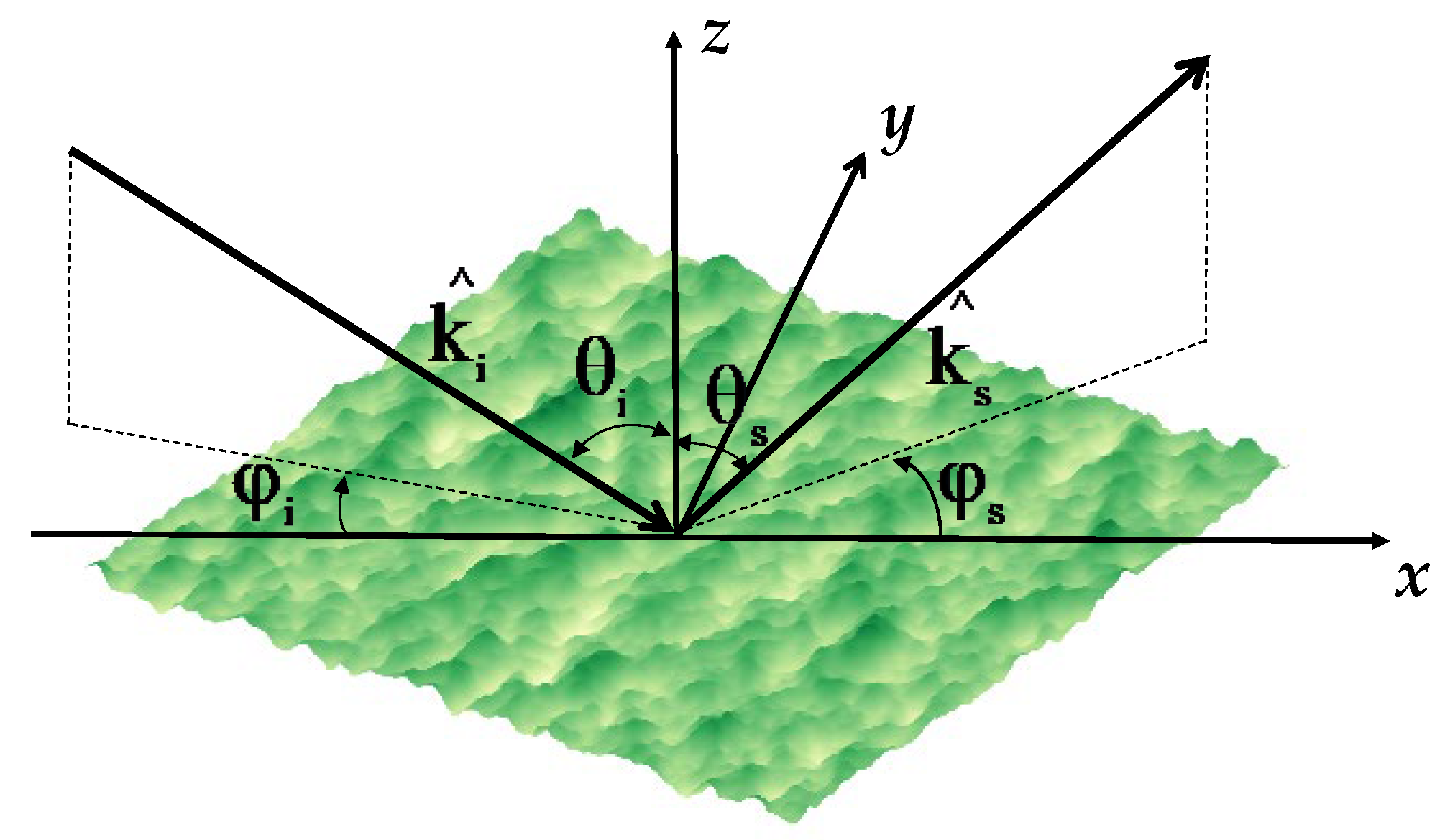
2. Materials and Methods

2.1. Experimental Data

In this study, the training data of the bi-directional network was obtained based on the mapping relationship between the surface parameters and radar observations. In fact, training data satisfying such conditions cannot be obtained from the point datasets measured in the field. The AIEM model can simulate the backscattering characteristics under various surface conditions. Given the range of variations in the surface permittivity, the root mean square height (RMS) height and correlation length of interest bi-directional neural network training data can be generated by the AIEM model [12,28].
The general formula of the AIEM model is shown in Figure 1.
σ q p ( s ) = σ q p k + σ q p k c + σ q p c
It can be seen that the scattering coefficient is composed of Kirchhoff terms σ q p k , cross terms σ q p k c and compensation terms σ q p c . The explicit form of AIEM can be given as
σ q p ( s ) = k 2 2 e σ 2 ( k s z 2 + k z 2 ) n = 1 σ 2 n n ! | I q p n | 2 S ( n ) ( k s x k x , k s y k y )
where k is the incident wave number, σ 2 represents the variance of the surface height and S n k s x k x , k s y k y denotes the surface roughness spectrum of the surface in terms of the nth power of the surface correlation function by two-dimensional Fourier transform.
As shown in Figure 1, the incident and scattered wave vectors can be defined as
k x = k sin θ i cos φ i     ; k y = k sin θ i sin φ i ; k z = k cos θ i
k s x = k sin θ s cos φ s     ; k s y = k sin θ s sin φ s ; k s z = k cos θ s
where θ i and φ i are the incident angle, and θ s and φ s are the scattering angle. The backscattering direction is at θ i = θ s , φ s = φ i + 180°.
POLARSCAT is a polarizing scatterometer that operates on different bare surfaces, each with wet and dry conditions. The polarimetric measurements are conducted at the L-, C- and X-band frequencies at incident angles ranging from 10° to 70°. In this paper, the experimental data in the L- (the center frequency is 1.5 GHz) and X-bands (the center frequency is 4.75 GHz) are selected. As shown in Table 1, three soils of different roughness were measured in dry and wet conditions. Where σ is the RMS height, l is the correlation length and k = 2 π / λ , ( λ = c / f , c = 3 × 10 8 ). The RMS height ranged from 0.40 cm to 1.12 cm, and the correlation length ranged from 8.4 cm to 9.9 cm. In [25,26,27], for the three surfaces (S1–S3), the measured autocorrelation function was found to be closer in shape to an exponential function.

2.2. Method

In this section, it will be introduced separately from the overall framework of the bi-directional network, the structure of the forward network and the structure of the reverse network. At the same time, the workflow of the bi-directional network will be introduced in detail.

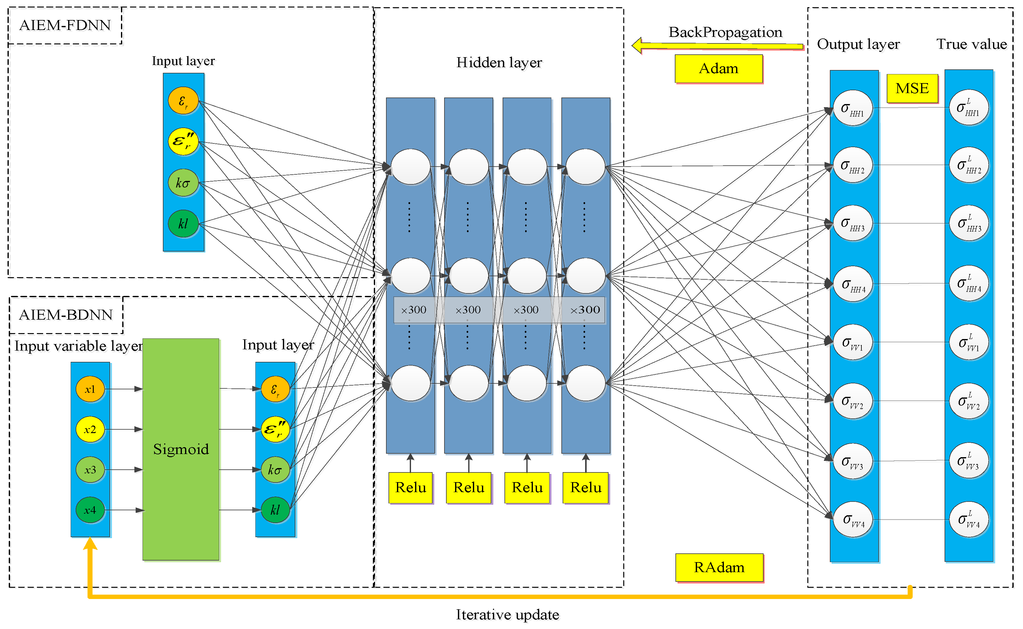
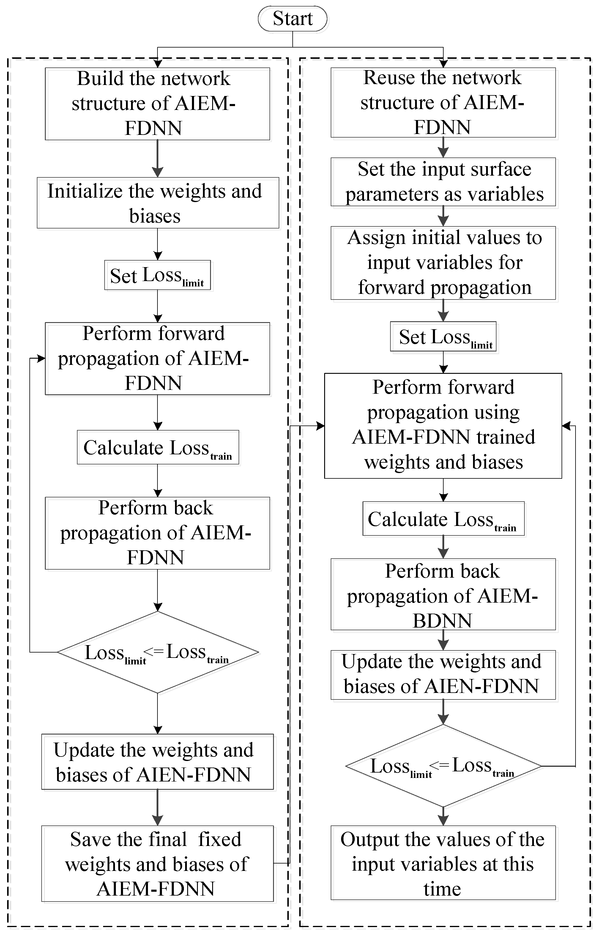
2.2.1. Framework of the Bi-Directional Deep Neural Network

There are usually two smart methods for solving inverse problems, namely the optimization algorithm and neural network inverse modeling method. The core idea of the optimization algorithm is to traverse the model space constructed by all parameters to obtain the optimal solution of the objective function. However, this kind of method needs to manually set the range of each parameter, and it is easy to fall into the local optimal solution when dealing with complex problems. In [29], a genetic algorithm was used to invert the surface parameters. It is often necessary to perform multiple searches to select the optimal solution, and the accuracy is not high. Another method is to use the backscattering coefficients as the input and the surface parameters as the output and use the neural network to directly construct the inverse model. However, since there is no exact analytical formula from the backscattering coefficients to the surface parameters, at the same time, the non-uniqueness of the dataset itself will make the overall training of the dataset difficult for the inverse model, thus affecting the inversion accuracy.
In this paper, a novel DNN-based surface parameters inversion method is proposed. As shown in Figure 2, this framework consists of two DNNs, namely an AIEM-Based Forward Deep Neural Network (AIEM-FDNN) and AIEM-Based Backward Deep Neural Network (AIEM-BDNN). The same network structure and weights are shared by them. The AIEM-FDNN takes the surface parameters as the input and the backscattering coefficients as the output. After training, it can be used to quickly calculate the backscattering coefficients outside the dataset. The AIEM-BDNN can be formed by reusing the network structure and well-trained weights of AIEM-FDNN. The input nodes need to be set as the variables. First, the input surface parameters are randomly initialized as constants. Then, the loss between the output backscattering coefficients and the actual backscattering coefficients will be calculated by the AIEM-BDNN. Finally, based on the back propagation of the error, the initialized surface parameters are continuously updated by the optimizer until the error converges into a sufficiently small value. Meanwhile, the updated surface parameters are the inversion results of the AIEM-BDNN based on this set of backscattering coefficients.
The flowchart of the overall working process of the bi-directional deep neural network is provided in Figure 3. The workflow of the AIEM-FDNN and AIEM-BDNN will be presented in detail in the following two parts.

2.2.2. AIEM-Based Forward Deep Neural Network

As shown in Figure 1, the AIEM-FDNN is a fully connected network that contains an input layer, multiple hidden layers and an output layer. Its input is the surface parameters, including the real part ε r and imaginary part ε r of the dielectric constant, the root mean square height k σ and the correlation length k l , and the output is the backscattering coefficients σ H H , σ V V .
The AIEM-FDNN is designed to calculate the backscattering coefficients. The trained AIEM-FDNN has similar computational accuracy to the AIEM model, and it is less complex to calculate. Since the AIEM-BDNN used for surface parameters inversion uses the network structure of AIEM-FDNN and the weights after training, the accuracy of the AIEM-FDNN directly affects the performance of the entire bi-directional DNN. The training process of the AIEM-FDNN consists of two stages: forward propagation and back propagation. The forward propagation is to calculate the loss of the output backscattering coefficients and the actual backscattering coefficients according to the current network weights. The back propagation is to update the weights using gradient descent techniques based on the current loss.
The forward propagation calculation process of AIEM-FDNN can be given as
Z A F 0 = [ ε r , ε r , k σ , k l ] A
Z A F i = g i W A F i Z A F i - 1 + b A F i i = 1 , , N
Z A F N = g N W A F N Z A F N - 1 + b A F N
[ σ H H , σ V V ] = Z A F N
where Z A F 0 and Z A F N represent the input surface parameters and the output backscattering coefficients for HH and VV polarizations for different incident angles, respectively. Z A F i i = 1 , , N represents the calculation result of the ith layer after the activation function. W A F i represents the weights matrix from the (i-1)th layer to the ith layer. b A F i represents the biases of the ith layer, and g i represents the nonlinear activation function of the ith layer. As shown in Figure 3, the calculated loss between the output backscattering coefficients and the actual backscattering coefficients will be calculated. The loss function of AIEM-FDNN is defined as the mean square error, which can be expressed as
L o s s A F = 1 n j = 1 n σ H H , j L σ H H , j 2 + σ V V , j L σ V V , j 2
where σ H H , j L , σ V V , j L represents the actual backscattering coefficients of the HH and VV polarization for the jth incident angle. The back propagation of AIEM-FDNN is based on the chain derivation rule. L o s s A F W A F i and L o s s A F b A F i are calculated to update W A F i and b A F i until L o s s A F converges to a minimum. The calculation process can be given as
E A F N = y l a b e l g N W A F N Z A F N - 1 + b A F N g N W A F N Z A F N - 1 + b A F N
E A F i = W A F i + 1 T E A F i + 1 g i W A F i Z A F i - 1 + b A F i
L o s s A F W A F i = E A F i Z A F i 1 T
L o s s A F b A F i = E A F i
where E A F N represents the error vector in the output layer of AIEM-FDNN, g i is the derivative of the activation function. E A F i is the error vector in the ith layer, and is the Hadamard product. Finally, the formulas for updating the weights and biases can be given as
W A F i = W A F i η A F L o s s A F W A F i
b A F i = b A F i η A F L o s s A F b A F i
where η A F represents the learning rate of the AIEM-FDNN.

2.2.3. AIEM-Based Backward Deep Neural Network

The AIEM-BDNN is constructed by directly reusing the network structure of the AIEM-FDNN and loading the training weights and biases to invert the surface parameters. Simply put, it is only necessary to set the input node of the trained AIEM-FDNN as variables. The training process of the AIEM-BDNN also includes forward propagation and back propagation, but it is different from the training object of AIEM-FDNN. The training objects of AIEM-FDNN are the weights and biases of the network, while the training objects of the AIEM-BDNN are the input surface parameters of the network. The AIEM-BDNN is trained by giving a set of backscattering coefficients to be inverted. By initializing the input surface parameters as constants, the forward propagation of the AIEM-BDNN is performed to calculate the backscattering coefficients. Back propagation is performed according to the loss between the output backscattering coefficients and the true backscattering coefficients. Finally, the initialized surface parameters are continuously updated until the loss converges to a small enough value. The last surface parameters updated are the inversion values.
The forward propagation calculation process of the AIEM-FDNN can be given as
Z A B 0 = [ ε r , ε r , k σ , k l ] B
Z A B i = g i W A F i Z A B i - 1 + b A F i i = 1 , , N
Z A B N = g N W A F N Z A B N 1 + b A F N
[ σ H H , σ V V ] = Z A B N
where [ ε r , ε r , k σ , k l ] B are randomly initialized surface parameters. W A F i represents the weights matrix from the (i-1)th layer to the ith layer of AIEM-FDNN. b A F i represents the biases of the ith layer of the AIEM-FDNN. Since the AIEM-FDNN has been trained, W A F i and b A F i have been fixed. They will not be updated in both the forward and backward propagation of the AIEM-BDNN. g i represents the nonlinear activation function of the ith layer of the AIEM-FDNN. Z A B i i = 1 , , N represents the calculation results of the ith layer of the AIEM-BDNN after the activation function. The loss function of the AIEM-BDNN is also defined as the mean squared error, which can be expressed as
L o s s A B = 1 n j = 1 n σ H H , j L σ H H , j 2 + σ V V , j L σ V V , j 2
The back propagation of the AIEM-BDNN is also based on the chain derivation rule. L o s s A B Z A B 0 is calculated to update Z A B 0 until L o s s A B converges to a minimum. The calculation process can be given as
E A B N = y l a b e l g N W A F N Z A B N 1 + b A F N g N W A F N Z A B N 1 + b A F N
E A B i = W A F i + 1 T E A B i + 1 g i W A F i Z A B i 1 + b A F i
L o s s A B Z A B 0 = ( W A F 1 ) T E A B 1
where E A B N represents the error vector in the output layer of the AIEM-BDNN, and g i is the derivative of activation function of AIEM-FDNN. E A B i is the error vector in the ith layer, and is the Hadamard product. Finally, the formulas for updating Z A B 0 can be given as
Z A B 0 = Z A B 0 η A B L o s s A B Z A B 0
in which η A B represents the learning rate of the AIEM-BDNN.
From the formula derivation of AIEM-FDNN and AIEM-BDNN, it can be seen that the training purpose of the AIEM-FDNN is to update the weights and biases of the network. Instead, AIEM-BDNN uses the weights and biases that AIEM-FDNN has already trained and fixed. Therefore, its training purpose is only to update the input parameters. It can be seen that the AIEM-FDNN and AIEM-BDNN are closely related. The quality of the AIEM-FDNN training will directly affect the inversion accuracy of the AIEM-BDNN. Therefore, using the bi-directional network to invert the surface parameters, we first need to ensure that the accuracy of the backscattering coefficients calculated by the AIEM-FDNN is high enough. The pseudocode of the bi-directional deep neural network was added as Appendix A to the article.

3. Results

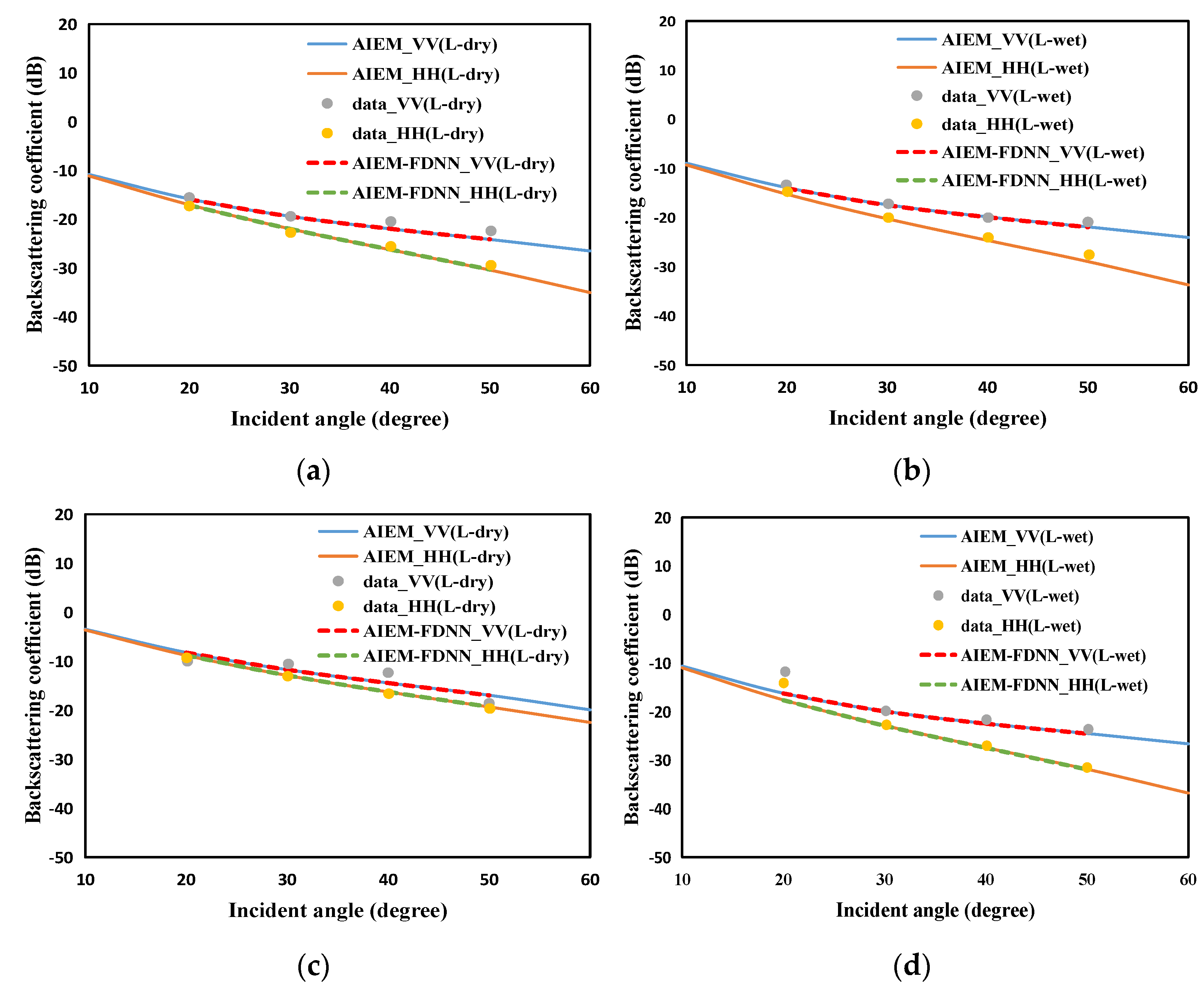
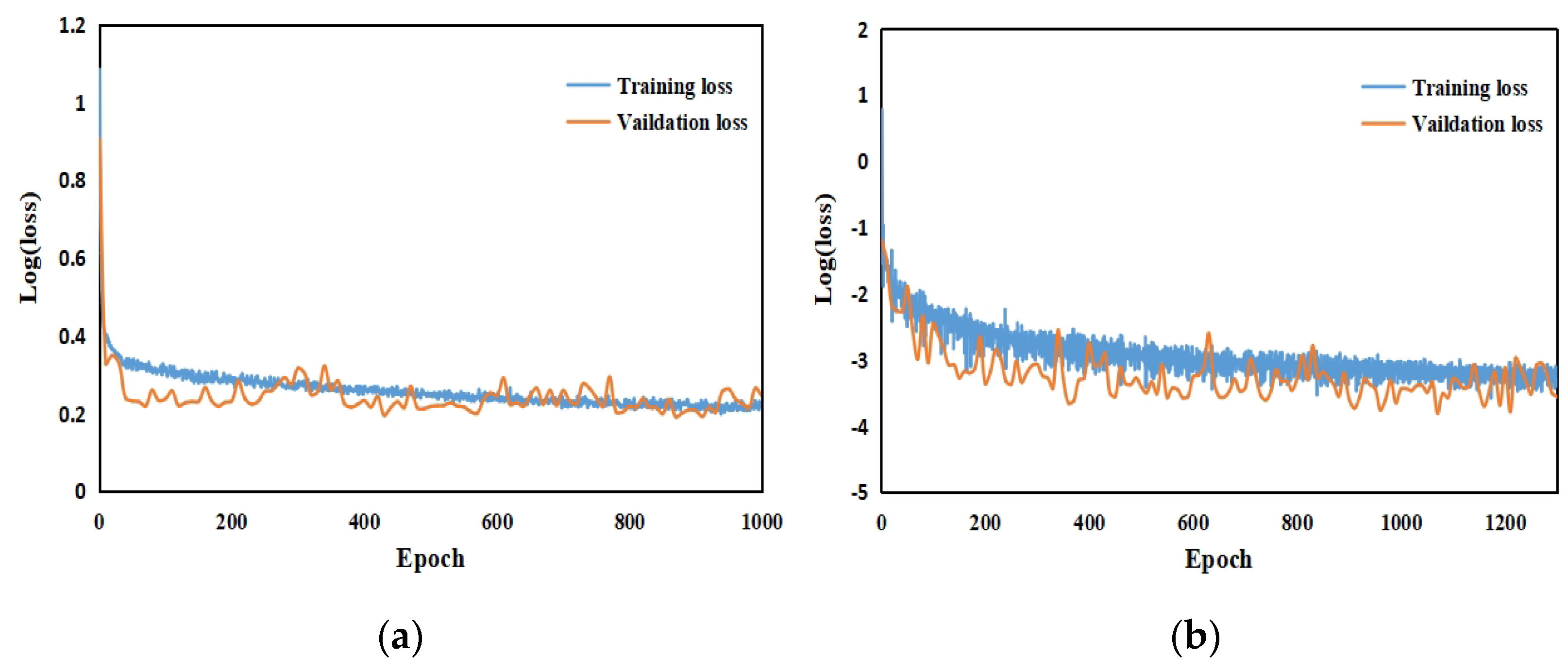
3.1. Performance of the AIEM-Based Forward Deep Neural Network

The selection of the datasets is crucial for the training of neural networks. Since the AIEM model can simulate the backscattering characteristics under various surface parameters, the training set required for the AIEM-FDNN can be generated as long as the variation range of the surface parameters is given. As shown in Table 2, the range of each surface parameter for generating the dataset is given. The range of the radar incident angle is set from 20° to 50°. Four surface parameters, namely the real and imaginary parts of the dielectric constant, the normalized root mean square height and the normalized correlation length, are used as the input of the AIEM-FDNN, while the backscattering coefficients for HH and VV polarization are the output. The sampling interval of the real part and imaginary part of the dielectric constant is 1.2 and 1, respectively. The sampling interval of the normalized root mean square height is 0.1. The normalized relative length is 0.7. A number of (21,009) sets of surface parameter combinations were generated by a cyclic combination within the range of surface parameters, and the corresponding backscattering coefficients were calculated by using the AIEM model. Many (3000) groups were selected as the validation set, and 1300 groups were selected as the test set.
Next, the AIEM-FDNN is built for forward prediction. After continuous testing and adjustment of the hyperparameters, the hyperparameter settings shown in Table 3 are finally determined. There are four hidden layers added in the AIEM-FDNN, and each layer has 300 neurons. The activation function of each hidden layer adopts the ReLU function. Then, using the mean squared error (MSE) as the loss function, the error between the output value and the true value for each epoch is calculated. At the same time, the popular optimizer Adam is used to realize the back propagation. Finally, the continuous updating of the weights and the biases can be realized. A decaying learning rate is used, so that the training loss can converge more smoothly. Setting the batch size to 20, the network converges when the epoch is equal to 1300.
The test set was used to test the ability of the AIEM-FDNN to predict backscattering coefficients. As shown in Table 4, the RMSE between the output backscattering coefficients for HH and VV polarizations for different incident angles and the actual backscattering coefficients for HH and VV polarizations for different incident angles can be reduced to be less than 0.1%. It can be seen that the training of the AIEM-FDNN is successful, and the accuracy is high. The trained AIEM-FDNN has almost the same computational accuracy as the AIEM model. The 21,009 sets of data generated by the AIEM model need 75.6 s, with 7.34 s for the proposed AIEN-FDNN. Therefore, the AIEM-FDNN has a faster computation speed when faced with a large amount of data generation tasks.
At the same time, the degree of agreement between the backscattering coefficients calculated by AIEM-FDNN and the measured data has a great influence on the accuracy of the bi-directional network inversion of actual surface parameters. POLARSCAT measured data are used to test the AIEM-FDNN. The comparison of backscattering coefficients of the AIEM (AIEM-VV and AIEM-HH), POLARSCAT measured data (data_VV and data_HH) and AIEM-FDNN (AIEM-FDNN_VV and AIEM-FDNN_HH) for exponential correlated surface are shown in Figure 4. It can be seen that the three have good consistency. This lays a good foundation for the AIEM-BDNN to invert POLARSCAT measured parameters.

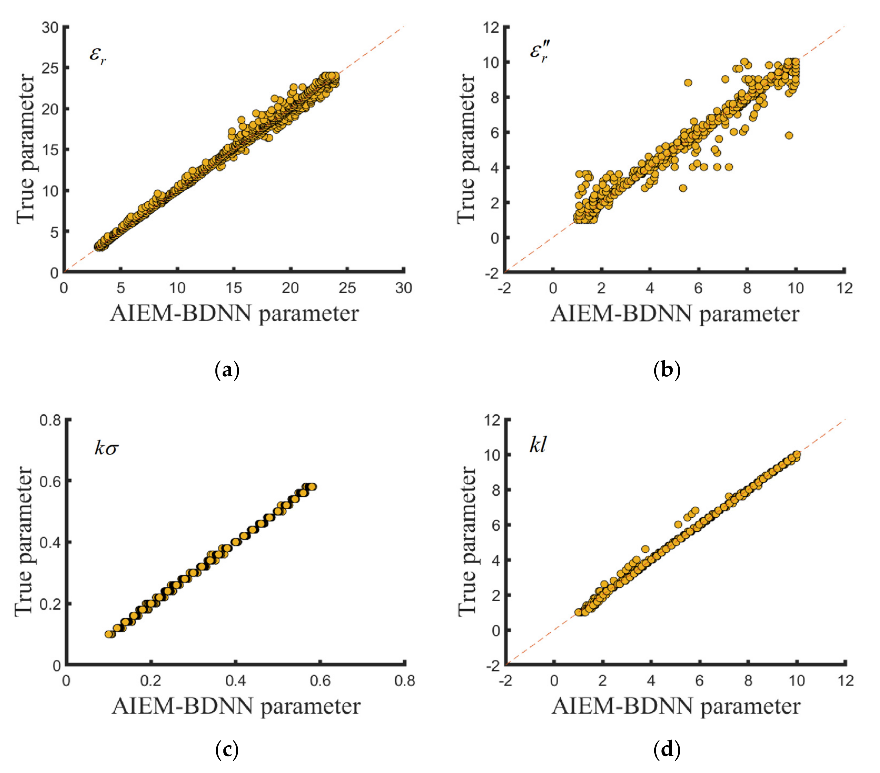
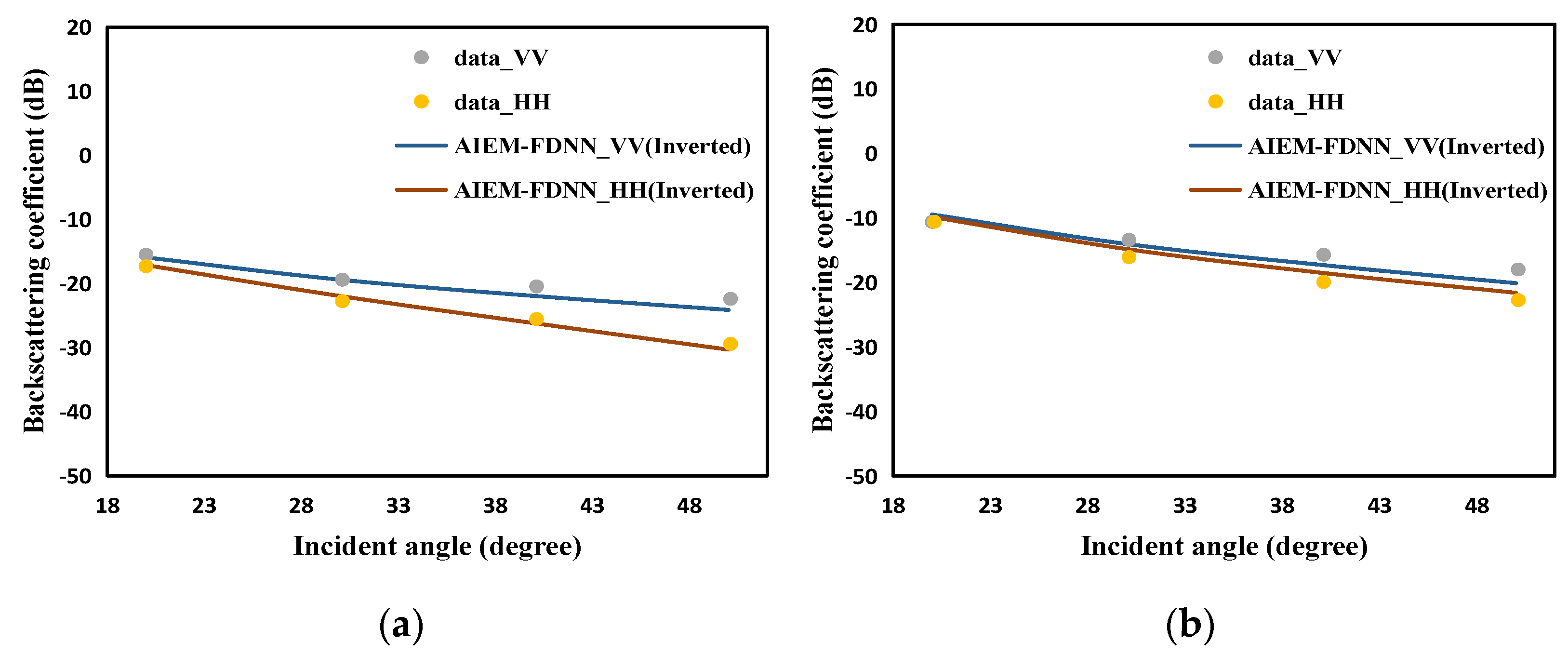
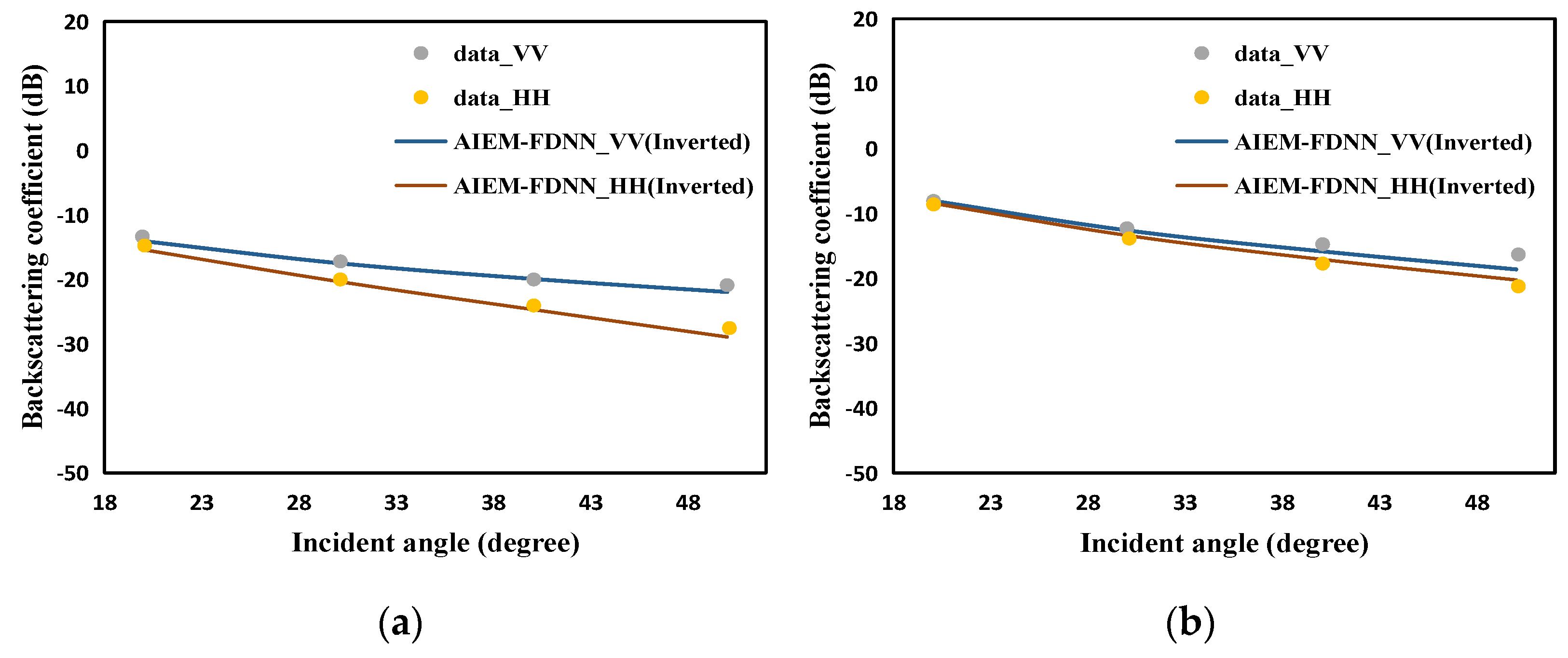
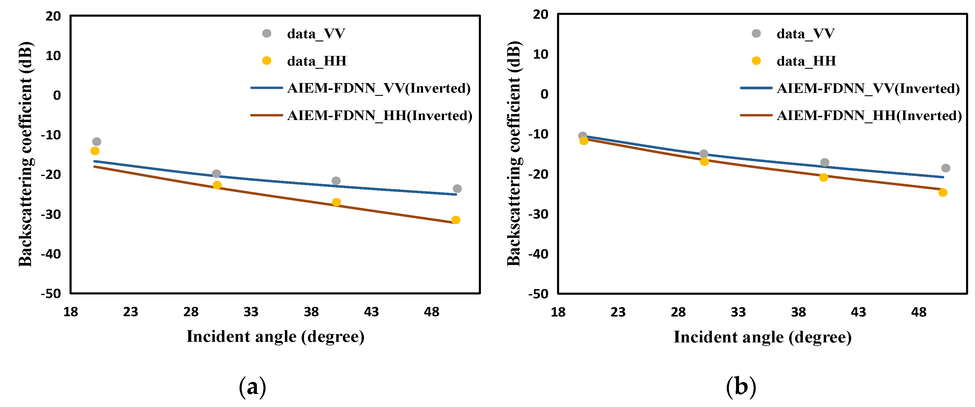
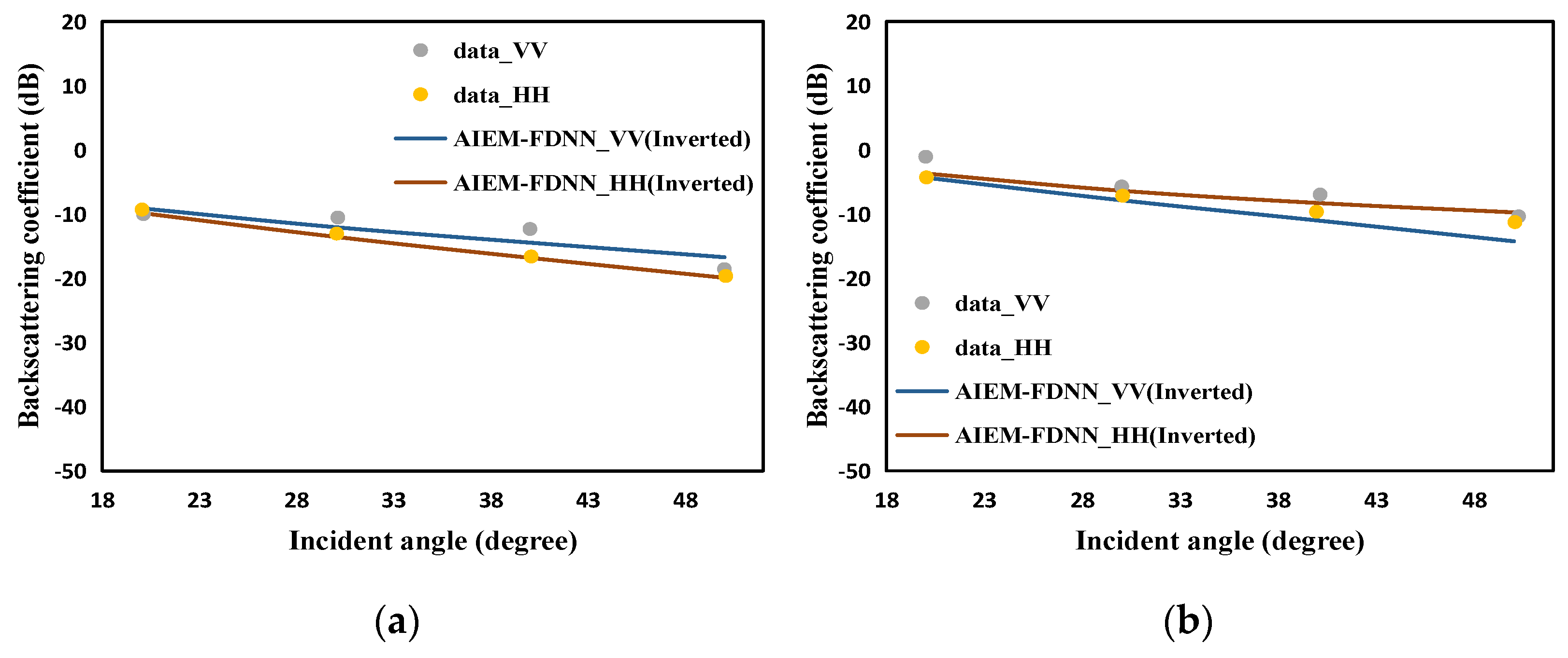
3.2. Performance of the AIEM-Based Backward Deep Neural Network

AIEM-BDNN is designed to complete the surface parameters inversion task. It can be established by reusing the network structure of the AIEM-FDNN and the well-trained weights and biases. It is worth noting that the weights and biases of the AIEM-FDNN have been fixed and will not change after being reused by the AIEM-BDNN. Simply put, only the input surface parameters of the AIEM-BDNN are updated during training. The hyperparameters used by the AIEM-FDNN are not suitable for the AIEM-BDNN. After continuous tuning, the RAdam optimizer was chosen instead of the Adam optimizer. Xavier Initialization is chosen as the initialization method of the input surface parameters.
Two outstanding problems were found in the experiments, one of which is that the surface parameters are not updated in the desired direction. As a result, although the training loss can converge normally, the surface parameters obtained by the final inversion often deviate from the conventional parameter space. The update of the surface parameters is not automatically limited to the respective data ranges shown in Table 2, and even negative values may appear. The reason for this is that the AIEM-BDNN can accept arbitrary update parameters due to the training mechanism of the DNN, and even the wrong parameter combination can calculate the same result as the real value. In order to limit the update range of the input surface parameters, before AIEM-FDNN training, the input surface parameters are normalized by the method of Min–Max_scale, and the parameters can be limited to 0–1. Next, a sigmoid layer is inserted between the input layer and the first hidden layer of AIEM-BDNN. As a commonly used nonlinear function, the sigmoid function can limit any input value between 0 and 1. In this way, you do not need the need to care whether the updated surface parameters are out of a reasonable range, because no matter how unreasonable the value of the updated surface parameter is, the sigmoid function will adjust it to the normal range. It should be noted here that, although the update object of the network is still the input surface parameters, the real input parameters of the AIEM-BDNN have become the values adjusted by the sigmoid function. At the same time, the value adjusted by the sigmoid function will also be used as the surface parameters inversed by AIEM-BDNN.
Another problem in the experiment is that there is a “premature” phenomenon when the input surface parameters are updating. This phenomenon is reflected in the fact that the training error cannot converge in the early stage of training. The reason is that, in the early stage of network training, the gradient decreases sharply, resulting in the slow update of neurons and ineffective learning. To alleviate such problem, the RAdam optimizer is used instead of the Adam optimizer, and the Xavier initialization method is used. The RAdam optimizer introduces a warm-up mechanism based on the commonly used Adam optimizer. Simply put, it is to use a small learning rate in the early stage of network training, so that the early training can be carried out smoothly and avoid excessive variance. The Xavier Initialization method will control the variance of the initial value within an appropriate range, usually making the variance of the initial value 1. It is also possible to choose to use the solution in [30,31]. By scanning all the variable hyperparameters in the AIEM-BDNN and recording the loss value, the one with the smallest loss is selected as the optimal inversion result. After continuous testing and adjustment of the hyperparameters, the hyperparameter settings shown in Table 5 are finally determined.
Many (1300) sets of test sets are used to examine the inversion accuracy of the AIEM-BDNN. As shown in Figure 5, the comparison of the true surface parameters and the AIEM-BDNN predicted surface parameters is given. The numerical results show that the predicted surface parameters and the true surface parameters are concentrated near the contour, which shows that the accuracy of the predicted parameters is high. The correlation coefficient between the two is calculated, respectively, 97.56% ( ε r ), 91.14% ( ε r ), 99.04% ( k σ ) and 98.45% ( k l ), as shown in Table 6.
As shown in Table 7, twelve sets of inversion results between POLARSCAT measured data and inverted by the AIEM-BDNN are compared. Three exponential distribution surfaces of POLARSCAT measured data are selected. As we can see, the comparison of the inversion results with the measured surface parameters can achieve satisfactory accuracy.
As shown in Figure 6, Figure 7, Figure 8, Figure 9, Figure 10, Figure 11 the inverted surface parameters are brought into the AIEM-FDNN. The obtained backscattering coefficients are compared with the measured values. It can be seen that the two have a good consistency.

4. Discussion

In this paper, the bi-directional network performs well in the task of surface parameter inversion. The bi-directional network has a high inversion accuracy for the AIEM model dataset. Similarly, for the inversion of the POLARSCAT measured data by the bi-directional network, the inversion value has a good correlation with the real value.
The bi-directional network is proposed to solve the problem of non-uniqueness, which leads to the poor effect of direct training of the inverse network. The nonunique data in the dataset itself will cause the training error of the directly constructed inverse network (with the backscattering coefficients as the input and the surface parameters as the output) to be unable to decrease and converge well. To solve this problem, bi-directional networks are proposed. The forward network AIEM-FDNN (with the surface parameters as the input and the backscattering coefficients as the output) is first trained, and the inverse network is constructed by reusing the weights trained by the AIEM-FDNN. In this way, the problem of directly constructing the inverse network can be avoided, and the bi-directional network achieves better inversion accuracy.
A BP (back propagation) neural network with backscattering coefficients as the input and surface parameters as the output is directly constructed. The 21,009 datasets generated by the AIEM model are used for training, and the training loss curve is shown in Figure 12a. Note that the training stops when the validation loss does not drop for 40 consecutive epochs. It can be seen that the training and validation losses for the BP neural network are 1.6257 and 1.5519, respectively, and the loss value barely dropped. This shows that the directly built inverse network performs poorly for the task of inverting surface parameters from input backscattering coefficients. The biggest reason that the inverse network cannot be trained well is the most common non-uniqueness problem in the inverse task of the neural network. Since the combination of different surface parameters can obtain the same or similar backscattering coefficients, this leads to a one-to-many situation during inverse network training. Once there are too many nonunique data in the dataset, the training loss of the network cannot be reduced well. On the contrary, the training of the forward network with the surface parameters as the input and the backscattering coefficient as the output does not have the influence of nonunique data on it. Therefore, it is hoped to start from the forward network and design a new method of surface parameter inversion. A bi-directional network was designed to overcome the above problems.
As shown in Figure 12b, the loss curve of training and validation converges to a small value and keeps fluctuating after the AIEM-FDNN trained for 1300 epochs. Finally, the training loss value and validation loss value of the network are 6.45 × 10 4 and 1.17 × 10 4 , respectively. This loss value of the proposed bi-directional DNN is smaller than the traditional inverse network by several magnitudes. The weights trained by the AIEM-FDNN can be directly reused by the AIEM-BDNN, which can show a better loss convergence. As shown in Table 8, the bi-directional network achieves a better inversion accuracy.

5. Conclusions

In this paper, a novel bi-directional neural network was proposed to invert the surface parameters. The establishment of the bi-directional network is divided into two steps. The AIEM-FDNN established first takes the surface parameters as the input and the backscattering coefficients as the output. The trained AIEM-FDNN can predict the backscattering coefficients outside the training dataset, and the predictions are also very accurate for the measured data. The AIEM-BDNN is built by reusing weights and biases trained by the AIEM-FDNN. At the same time, it is necessary to give the input surface parameter initialization constants, and a sigmoid layer between the input layer and the first hidden layer is inserted. After the error between the output backscattering coefficients and the true backscattering coefficients is continuously reduced, the input surface parameters can be continuously updated. The numerical results show that the bi-directional network not only has a good inversion effect for the data in the dataset but also has a high inversion accuracy for the measured data outside the dataset.
The bi-directional network is divided into a forward network (AIEM-FDNN) and an inverse network (AIEM-BDNN). The AIEM-BDNN is constructed by reusing the weights and biases of the AIEM-FDNN and does not require secondary training. Therefore, the training accuracy of the AIEM-FDNN will directly determine the inversion accuracy of the AIEM-BDNN. If the training effect of the forward network on some datasets is not good, then the bi-directional network will not be able to achieve a good inversion result.
One limitation we had to deal with in this paper is that the datasets used were only for backscattering coefficients under HH and VV polarizations. As a future work direction, we plan to incorporate the backscattering coefficients under HV and VH polarizations. The more abundant features of the four polarizations were used to further improve the accuracy of the surface parameters inversion. In addition, we considered adding part of the measured data to the dataset generated by the AIEM for training. We hope to reduce some of the differences between the simulated and measured data.

Author Contributions

Conceptualization, Y.W. and Z.H.; methodology, Y.W. and Z.H.; software, Y.W.; validation, Y.W., Z.H. and Y.Y.; formal analysis, Y.W., Z.H., Y.Y., D.D., F.D. and X.-W.D.; investigation, Y.W.; resources, Y.W. and Z.H.; data curation, Y.W.; writing—original draft preparation, Y.W.; writing—review and editing, Y.W., Z.H., Y.Y., D.D., F.D. and X.-W.D.; visualization, Y.W.; supervision, Z.H.; project administration, Z.H. and funding acquisition, Z.H. All authors have read and agreed to the published version of the manuscript.

Funding

This work was supported in part by Natural Science 62071231, 61890541 and 61931021; Jiangsu Province Natural Science Foundation under Grant BK20211571 and the Fundamental Research Funds for the Central Universities of No. 30921011207, Laboratory of Pinghu (Beijing Institute of infinite electric Measurement), Science and Technology on Electromagnetic Scattering Laboratory.

Data Availability Statement

No applicable.

Conflicts of Interest

The authors declare no conflict of interest.

Appendix A

Algorithm A1: Bi-directional Deep Neural Network
Input: The input surface parameters Z A F 0 and Z A B 0 , the true backscattering coefficients [ σ H H L , σ V V L ] , the maximum epoch I, the weights matrix W A F i and W A B i , the bias vector b A F i and b A B i , the nonlinear activation function g i , the loss function MSE, the learning rate η A F ,   η A B
1: initialize W A F i and b A F i
2: for j = 1; jI do
3:   Z A F i = g i W A F i Z A F i - 1 + b A F i i = 1 , , N
4:   Z A F N = g N W A F N Z A F N 1 + b A F N
5:   L o s s A F = M S E Z A F N , [ σ H H L , σ V V L ]
6:   W A F i = W A F i η A F L o s s A F W A F i , b A F i = b A F i η A F L o s s A F b A F i
7:  if L o s s A F convergence then
8:   break loop
9:  end if
10:  j = j + 1
11: end for
12: return W A F i and b A F i
13: Initialize Z A B 0
14: for k = 1; kI do
15:   Z A B i = g i W A F i Z A B i 1 + b A F i i = 1 , , N
16:   16 :   Z A B N = g N W A F N Z A B N - 1 + b A F N
17:   L o s s A B = M S E Z A B N , [ σ H H L , σ V V L ]
18:   Z A B 0 = Z A B 0 η A B L o s s A B Z A B 0
19:  if L o s s A B convergence then
20:   break loop
21:  end if
22:  k = k + 1
23: end for
24: return Z A B 0
Output: Inversion results Z A B 0

References

  1. Mohammad, H.M.; Amir, A.; Hamid, S.S. Substitution of satellite-based land surface temperature defective data using GSP method. Adv. Space Res. 2021, 67, 3106–3124. [Google Scholar]
  2. Kim, Y.; Jackson, T.; Bindlish, R.; Lee, H.; Hong, S. Monitoring soybean growth using L-, C- and X-band scatterometer data. Int. J. Remote Sens. 2013, 34, 4069–4082. [Google Scholar] [CrossRef]
  3. Yang, H.; Guo, H.D.; Wang, C.L.; Li, X.W.; Yue, H.Y. Polarimetric SAR surface parameters inversion based on network. J. Remote Sens. 2002, 6, 451–455. [Google Scholar]
  4. Shen, X.; Mao, K.; Qin, Q.; Hong, Y.; Zhang, G. Bare surface soil moisture estimation using double-angle and dual-polarization L-band radar data. IEEE Trans. Geosci. Remote Sens. 2013, 51, 3931–3942. [Google Scholar] [CrossRef]
  5. Chiang, C.Y.; Chen, K.S.; Yang, Y.; Wang, S.Y. Computation of backscattered fields in polarimetric SAR imaging simulation of complex targets. IEEE Trans. Geosci. Remote Sens. 2022, 60, 2004113. [Google Scholar] [CrossRef]
  6. Sancer, M. Modified Beckmann-Kirchhoff scattering model for rough surface with large incident and scattering angles. Opt. Eng. 2007, 46, 078002. [Google Scholar]
  7. Thorsos, E.I. The validity of the perturbation approximation for rough surface scattering using a Gaussian roughness spectrum. Acoust. Soc. Am. 1989, 86, 261–277. [Google Scholar] [CrossRef]
  8. Soto-Crespo, J.M.; VesPerinas, M.N.; Friberg, A.T. Scattering from slightly rough random surfaces: A detailed study on the validity of the small perturbation method. J. Opt. Soc. Am. A 1990, 7, 1185–12017. [Google Scholar] [CrossRef] [Green Version]
  9. Gilbert, M.S.; Johnson, M.S. A study of the higher-order small-slope approximation for scattering from a Gaussian rough surface. Waves Random Media 2003, 13, 137–149. [Google Scholar] [CrossRef]
  10. Berginc, G.; Bourrely, C. The small-slope approximation method applied to a three-dimensional slab with rough boundaries. Prog. Electromagn. Res. 2007, 73, 131–211. [Google Scholar] [CrossRef] [Green Version]
  11. Xu, F.; Jin, Y.Q. Imaging simulation of po-larimetric SAR for a comprehensive terrain scene using the mapping and projection algorithm. IEEE Trans. Geosci. Remote Sens. 2006, 44, 3219–3234. [Google Scholar] [CrossRef]
  12. Zeng, J.Y.; Chen, K.S.; Bi, H.Y.; Zhao, T.J.; Yang, X.F. A comprehensive analysis of rough soil surface scattering and emission predicted by AIEM with comparison to numerical simulations and experimental measurements. IEEE Trans. Geosci. Remote Sens. 2017, 55, 1696–1708. [Google Scholar] [CrossRef]
  13. Chen, K.S.; Wu, T.D.; Tsang, L.; Li, Q.; Shi, J.; Fung, A.K. Emission of rough surfaces calculated by the integral equation method with comparison to three-dimensional moment method simulations. IEEE Trans. Geosci. Remote Sens. 2003, 41, 90–101. [Google Scholar] [CrossRef]
  14. Ulaby, F.T.; Sarabandi, K.; Mcdonald, K.Y.L.E.; Whitt, M.; Dobson, M.C. Michigan microwave canopy scattering model. Int. J. Remote Sens. 1990, 11, 1223–1253. [Google Scholar] [CrossRef]
  15. Dubois, P.; Van Zyl, J.; Engman, T. Measuring soil moisture with imaging radars. IEEE Trans. Geosci. Remote Sens. 1995, 33, 915–926. [Google Scholar] [CrossRef] [Green Version]
  16. Oh, Y. Quantitative retrieval of soil moisture content and surface roughness from multipolarized radar observations of bere soil surfaces. IEEE Trans. Geosci. Remote Sens. 2004, 42, 596–601. [Google Scholar] [CrossRef]
  17. Zhao, S.T. Inverse calculation of hydrogeological parameters in Henan based on improved genetic algorithm. Ground Water 2019, 41, 77–79. [Google Scholar]
  18. Wang, L.X.; Wang, A.Q.; Huan, Z.X. Parameter inversion of rough surface optimization based on multiple algorithms for SVM. Chin. J. Comput. Phys. 2019, 36, 577–585. [Google Scholar]
  19. Peurifoy, J.; Shen, Y.; Jing, L.; Yang, Y.; Cano-Renteria, F.; DeLacy, B.G.; Joannopoulos, J.D.; Tegmark, M.; Soljačić, M. Nanophotonic particle simulation and inverse design using artificial neural networks. Sci. Adv. 2018, 4, eaar4206. [Google Scholar] [CrossRef] [Green Version]
  20. Li, G.; Li, X.Z.; Liu, D.J.; Wang, L.H.; Yu, Z.F. A bidirectional deep neural network for accurate silicon color design. Adv. Mater. 2019, 31, 1905467. [Google Scholar]
  21. Xu, F.; Wang, H.P.; Jin, Y.Q. Deep learning as applied in SAR target recognition and terrain classification. J. Radars 2017, 6, 136–148. [Google Scholar]
  22. Sharifzadeh, F.; Akbarizadeh, G.; Kavian, Y.S. Ship classification in SAR images using a new hybrid CNN-MLP classifier. J. Indian Soc. Remote Sens. 2019, 47, 551–562. [Google Scholar] [CrossRef]
  23. Ding, J.; Chen, B.; Liu, H.W.; Huang, M.Y. Convolutional Neural Network with Data Augmentation for SAR Target Recognition. IEEE Geosci. Remote Sens. Lett. 2016, 13, 364–368. [Google Scholar] [CrossRef]
  24. Niu, S.R.; Qiu, X.L.; Lei, B.; Ding, C.B.; Fu, K. Parameter extraction based on deep neural network for SAR target simulation. IEEE Trans. Geosci. Remote Sens. 2020, 58, 4901–4914. [Google Scholar] [CrossRef]
  25. Oh, Y.; Sarabandi, K.; Ulaby, F.T. An empirical model and inversion technique for radar scattering from bare soil surfaces. IEEE Trans. Geosci. Remote Sens. 1992, 30, 370–381. [Google Scholar] [CrossRef]
  26. Yang, Y.; Chen, K.S.; Shang, G.F. Surface parameters retrieval from fully bistatic radar scattering data. Remote Sens. 2019, 11, 596. [Google Scholar] [CrossRef] [Green Version]
  27. Chen, K.S. Radar Scattering and Imaging of Rough Surfaces, 1st ed.; CRC Press: Boca Raton, FL, USA, 2021; pp. 160–163. [Google Scholar]
  28. Yang, Y.; Chen, K.S.; Tsang, L.; Yu, L. Depolarized backscattering of rough surface by AIEM model. IEEE J. Sel. Top. Appl. Earth Sci. Remote Sens. 2017, 10, 4740–4752. [Google Scholar] [CrossRef]
  29. Zhang, Y.Y.; Wu, Z.S.; Zhang, Y.S. The effective permittivity and roughness parameters inversion by the land backscattering measured data. Chin. J. Radio Sci. 2016, 31, 79–84. [Google Scholar]
  30. So, S.; Badloe, T.; Noh, J.; Bravo-Abad, J.; Rho, J. Deep learning enable inverse design in nanophotonics. Nanophotonics 2020, 9, 1041–1057. [Google Scholar] [CrossRef] [Green Version]
  31. Li, J.; Li, X.Z.; Wu, Q.X.; Wang, L.H.; Li, G. Neural network enabled metasurface design for phase manipulation. Opt. Express 2021, 29, 2521–2528. [Google Scholar]
Figure 1. Schematic diagram of scattering from rough surfaces.
Remotesensing 14 03302 g001
Figure 2. The framework for the proposed AIEM-based bi-directional deep neural network.
Remotesensing 14 03302 g002
Figure 3. Flowchart of the working process of the bi-directional DNN.
Remotesensing 14 03302 g003
Figure 4. Comparison of backscattering coefficients of the AIEM, POLARSCAT measured data and AIEM−FDNN for exponential correlated surface with (a) ε r = 7.99, ε r = 2.02, k σ = 0.13 and k l = 2.6 at 1.5 GHz; (b) ε r = 15.57, ε r = 3.71, k σ = 0.13 and k l = 2.6 at 1.5 GHz; (c) ε r = 7.7, ε r = 1.95, k σ = 0.35, k l = 2.6 at 1.5 GHz and (d) ε r = 14.43, ε r = 3..47, k σ = 0.1 and k l = 3.1 at 1.5 GHz.
Remotesensing 14 03302 g004
Figure 5. Comparison of true parameters and the AIEM−BDNN predicted parameters for: (a) the real part of the dielectric constant, (b) the imaginary part of the dielectric constant, (c) the normalized root mean square height and (d) the normalized correlation length.
Remotesensing 14 03302 g005
Figure 6. Comparison of the backscattering coefficients of the AIEM, POLARSCAT measured data and AIEM−FDNN for exponential correlated surfaces with (a) measured: ε r = 7.99, ε r = 2.02, k σ = 0.13 and k l = 2.6 at 1.5 GHz; inverted: ε r = 9.07, ε r = 1.23, k σ = 0.13 and k l = 2.81; (b) measured: ε r = 8.77, ε r = 1.04, k σ = 0.4 and k l = 8.4 at 4.75 GHz; inverted: ε r = 9.33, ε r = 1.19, k σ = 0.40 and k l = 8.49.
Remotesensing 14 03302 g006
Figure 7. Comparison of the backscattering coefficients of the AIEM, POLARSCAT measured data and AIEM−FDNN for the exponential correlated surface with (a) measured: ε r = 15.57, ε r = 3.71, k σ = 0.13, and k l = 2.6 at 1.5 GHz; inverted: ε r = 15.19, ε r = 4.09, k σ = 0.13 and k l = 2.79; (b) measured: ε r = 15.42, ε r = 2.15, k σ = 0.40 and k l = 8.4 at 4.75 GHz; inverted: ε r = 16.00, ε r = 0.36, k σ = 0.40 and k l = 8.44.
Remotesensing 14 03302 g007
Figure 8. Comparison of backscattering coefficients of the AIEM, POLARSCAT measured data and AIEM−FDNN for the exponential correlated surface with (a) measured: ε r = 5.85, ε r = 1.46, k σ = 0.10 and k l = 3.1 at 1.5 GHz; inverted: ε r = 3.02, ε r = 2.96, k σ = 0.16 and k l = 1.29; (b) measured: ε r = 6.66, ε r = 0.68, k σ = 0.32 and k l = 9.8 at 4.75 GHz; inverted: ε r = 3.23, ε r = 0.95, k σ = 0.36 and k l = 1.00.
Remotesensing 14 03302 g008
Figure 9. Comparison of the backscattering coefficients of the AIEM, POLARSCAT measured data and AIEM−FDNN for the exponential correlated surface with (a) measured: ε r = 14.43, ε r = 3.47, k σ = 0.10 and k l = 3.1 at 1.5 GHz; inverted: ε r = 10.58, ε r = 5.43, k σ = 0.10 and k l = 3.09; (b) measured: ε r = 14.47, ε r = 1.99, k σ = 0.32 and k l = 9.8 at 4.75 GHz; inverted: ε r = 14.91, ε r = 1.63, k σ = 0.32 and k l = 9.88.
Remotesensing 14 03302 g009
Figure 10. Comparison of the backscattering coefficients of the AIEM, POLARSCAT measured data and AIEM−FDNN for the exponential correlated surface with (a) measured: ε r = 7.77, ε r = 1.95, k σ = 0.35 and k l = 2.6 at 1.5 GHz; inverted: ε r = 7.41, ε r = 2.53, k σ = 0.31 and k l = 1.89; (b) measured: ε r = 8.5, ε r = 1.00, k σ = 1.11 and k l = 8.4 at 4.75 GHz; inverted: ε r = 9.34 ε r = 0.42, k σ = 0.99 and k l = 6.66.
Remotesensing 14 03302 g010
Figure 11. Comparison of the backscattering coefficients of the AIEM, POLARSCAT measured data and AIEM−FDNN for the exponential correlated surface with (a) measured: ε r = 15.34, ε r = 3.66, k σ = 0.35 and k l = 2.6 at 1.5 GHz; inverted: ε r = 20.79, ε r = 4.49, k σ = 0.32 and k l = 1.04; (b) measured: ε r = 15.23, ε r = 2.12, k σ = 1.11 and k l = 8.4 at 4.75 GHz; inverted: ε r = 15.00, ε r = 4.58, k σ = 0.99 and k l = 8.86.
Remotesensing 14 03302 g011
Figure 12. (a) Learning curve of the BP neural network. (b) Learning curve of the AIEM−FDNN.
Remotesensing 14 03302 g012
Table 1. POLARSCAT measured parameters.
Surface NumberFreq. (GHz) k σ k l σ (cm) l (cm) ε r ε r
S1-dry1.5 GHz0.132.60.408.47.992.02
4.75 GHz0.48.48.771.04
S1-wet1.5 GHz0.132.615.573.71
4.75 GHz0.48.415.422.15
S2-dry1.5 GHz0.13.10.329.95.851.46
4.75 GHz0.329.86.660.68
S2-wet1.5 GHz0.13.114.433.47
4.75 GHz0.329.814.471.99
S3-dry1.5 GHz0.352.61.128.47.701.95
4.75 GHz1.118.48.501.00
S3-wet1.5 GHz0.352.615.343.66
4.75 GHz1.118.415.232.12
Table 2. Surface parameters and radar parameters.
ParameterValue
Real part of the dielectric constant ( ε r )2–26
Imaginary part of the dielectric constant   ( ε r )0.1–10.1
Normalized root mean square height   height   ( k σ )0.1–1
Normalized relative lenght   ( k l )1–10.8
Range of incident angle   ( θ i ) 20 50
Polarization modeHH, VV
k σ / k l 0.01–0.5
ε r / ε r 0–0.5
Surface roughness spectrum (S)Exponential
Table 3. Training the hyperparameters of the AIEM-FDNN.
ParameterValue
Weight initialization methodUniform distribution initialization
Activation functionReLU
Loss functionMSE
OptimizerAdam
Learning rate0.001
Learning decay rate0.9
Hidden layers4
Hidden neurons300
Epoch1300
Batch size20
Table 4. The RMSE between the output backscattering coefficients and the actual backscattering coefficients for the proposed AIEM-FDNN with φ = 0 180 .
Polarization
Incident   Angle   ( θ )
RMSE
VV20°0.1055%
VV30°0.0585%
VV40°0.0557%
VV50°0.0708%
HH20°0.0905%
HH30°0.0589%
HH40°0.0661%
HH50°0.0655%
Table 5. Training hyper-parameters of AIEM-BDNN.
ParameterValue
Input value initialization methodXavier Initialization
Activation functionReLU
Loss functionMSE
OptimizerRAdam
Learning rate0.001
Learning decay rate0.9
Hidden layers4
Hidden neurons300
Epoch10,000
Table 6. Inversion accuracy of the bi-directional neural networks.
ParameterRMSESimilarity(1-RMSE)
ε r 0.024497.56%
ε r 0.088691.14%
k σ 0.009699.04%
k l 0.015598.45%
Table 7. Comparison of the surface parameters between POLARSCAT measured data and inverted by the AIEM-BDNN.
Surface NumberPOLARSCAT (Measured)AIEM-BDNN (Inverted)
ε r ε r k σ k l ε r ε r k σ k l
S1-dry7.992.020.132.69.071.230.132.81
8.771.040.408.49.331.190.408.49
S1-wet15.573.710.132.615.194.090.132.79
15.422.150.408.416.000.360.408.44
S2-dry5.851.460.103.13.022.960.161.29
6.660.680.329.83.230.950.361.00
S2-wet14.433.470.103.110.585.430.103.09
14.471.990.329.814.911.630.329.88
S3-dry7.71.950.352.67.412.530.311.89
8.51.001.118.49.340.420.996.66
S3-wet15.343.660.352.620.794.490.321.04
15.232.121.118.415.004.580.998.86
ε r ε r k σ k l
RMSE2.361.210.0552.69
nRMSE0.13280.23860.06170.3029
Table 8. Inversion accuracy of BP neural networks and Bi-directional DNN.
Bi-Directional DNNBP
ParameterRMSESimilarity
(1-RMSE)
RMSESimilarity
(1-RMSE)
ε r 0.024497.56%0.052894.72%
ε r 0.088691.14%0.494850.52%
k σ 0.009699.04%0.045795.43%
k l 0.015598.45%0.037496.26%
Publisher’s Note: MDPI stays neutral with regard to jurisdictional claims in published maps and institutional affiliations.

