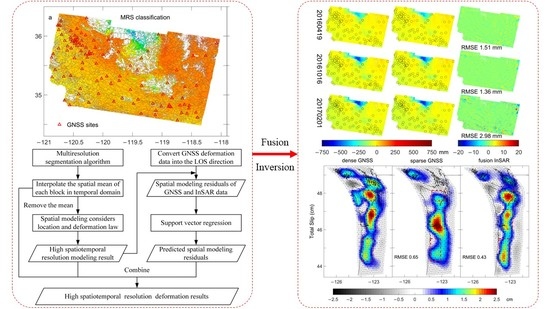
Fusion of Spatially Heterogeneous GNSS and InSAR Deformation Data Using a Multiresolution Segmentation Algorithm and Its Application in the Inversion of Slip Distribution

Abstract

The fusion of global navigation satellite system (GNSS) and interferometric synthetic aperture radar (InSAR) deformation data can leverage the advantages of GNSS high temporal resolution and InSAR high spatial resolution, and obtain more abundant deformation data for constraints on geophysical structural and mechanical parameters. Existing studies seldom consider the spatial heterogeneity of largescale deformation data, which easily leads to obvious spatial aggregation of errors in the results of fusion. Here, we propose a novel multiresolution segmentation fusion (MRSF) method that uses a multiresolution segmentation algorithm to automatically classify the spatial heterogeneity of InSAR deformation data with similar deformation characteristics. We applied the MRSF method to the fusion of GNSS and InSAR deformation data covering the central valley aquifer system (CVAS) in southern California to verify its precision and robustness. Results show that the MRSF method can accurately reflect spatiotemporal evolution characteristics of displacement data and reliably estimate deformation for the times and locations of missing data. We then tested this method for geophysical parameter estimation by constructing three different sets of data, including dense GNSS sites, sparse GNSS sites, and sparse GNSS sites fused with InSAR data using MRSF, to invert the slip distribution of the Cascadia subduction zone. Results show that the inverted slip of the fused InSAR and GNSS data is comparable to that of the dense GNSS sites. Therefore, the MRSF method can obtain deformation results with high precision and high spatiotemporal resolution and effectively compensate for the lack of data caused by sparse GNSS sites during the geophysical inversion process.

1. Introduction

Deformation data with high spatiotemporal resolution and precision are important for geohazard monitoring [1,2] and geophysical source inversion [3]. The global navigation satellite system (GNSS) has the advantages of high precision and high temporal resolution. However, owing to the high cost of deployment and maintenance, the spatial resolution of current GNSS sites in most regions of the world remains low. Even in California (http://sopac-csrc.ucsd.edu/index.php/crtn/, accessed on 14 September 2021), where GNSS sites are densely distributed, their spatial resolution is only 10–20 km [4]. On the other hand, interferometric synthetic aperture radar (InSAR) has a high spatial resolution (tens of meters) but relatively poor temporal resolution due to the infrequent satellite revisit time, and contains various sources of noise that are not present in GNSS or have been stably corrected with the years of development of GNSS technology [5].

Fusing GNSS and InSAR data leverages the strength of each dataset and enables deformation data with higher spatiotemporal resolution. Liu et al. [6] applied the spatiotemporal random effects (STRE) model to the fusion of GNSS and InSAR deformation data, but they did not consider the spatial heterogeneity of the deformation data, resulting in regional spatial clustering errors. Shi et al. [7] added spatial heterogeneity constraints to the STRE model, improving the accuracy of results of data fusion, but relied on external prior information to obtain the extent of spatially heterogeneous regions. Yan et al. [8] established a method to automatically determine the optimal location of the spatial bases, which improved the reliability and applicability of the STRE model, but was less effective for deformation data fusion with obvious spatial heterogeneity. In general, none of these methods of fusion of GNSS and InSAR deformation data can automatically characterize spatially heterogeneous information in them.

Existing studies have shown that spatiotemporal evolution characteristics of deformation in different regions are related to specific environmental and medium properties, which often results in largescale deformation of signals exhibiting notable spatial heterogeneity. Examples of this heterogeneity include uneven surface uplift and subsidence caused by oil and gas exploitation [9], seasonal settlement and uplift from farmland groundwater pumping and irrigation [10], and periodic irregular land reclamation caused by sediment compaction [11]. Therefore, in the process of fusing GNSS and InSAR deformation data, it is necessary to automatically identify heterogeneous objects according to spatiotemporal evolution characteristics of deformation data and assist the fusion model in performing more targeted processing to reduce the spatial aggregation of fusion errors, thereby improving accuracy and applicability.

Here, we focus on addressing the consideration of spatial heterogeneity in the fusion method and the application of its results to the inversion of geophysical parameters. In this paper, we first introduce our method for the fusion of GNSS and InSAR deformation data that automatically accounts for spatial heterogeneity. Next, we apply the method for the fusion of GNSS and InSAR deformation data in the central valley aquifer system (CVAS) with a large deformation magnitude, high spatial heterogeneity, and dense data coverage, and evaluate the resulting accuracies through a comparison with independent GNSS and InSAR data. Then, we apply the fusion method to the inversion of slip distribution in the Cascadia subduction zone with a high risk of ultra-strong earthquakes and assess experimental results by comparing them with previous estimates. Finally, we summarize the key features and advantages of this fusion method.

2. Methods

The multiresolution segmentation fusion (MRSF) method divides the deformation field into three parts: spatial mean, results of spatial modeling, and residuals of spatial modeling. The MRSF method first unifies the framework of GNSS and InSAR deformation data, then uses the multiresolution segmentation (MRS) algorithm [12,13] to extract the characteristic spatial distribution of deformation in InSAR data and form featured blocks/patches through clustering adjacent sites with similar deformation characteristics (Figure 1). Fourier curve fitting [14] was performed on the spatial mean of each block in the temporal domain to obtain the spatial mean of each block at each observation moment because it has good performance on data with certain temporal repeating patterns. Next, the demeaned deformation data were spatially modeled by combining the enhanced inverse-distance weighting method [15] and the least squares method [16] to consider the spatial location of the site and its deformation characteristics. Finally, support vector regression (SVR) [17] was used to estimate the residuals of spatial modeling in both the temporal and spatial domains and obtain deformation results with high precision and high spatiotemporal resolution.

2.1. Framework for the Unification of GNSS and InSAR Data

Because GNSS data provide information on deformations in the north, east, and vertical directions relative to a fixed framework, and InSAR data provide information on a one-dimensional deformation along the line-of-sight (LOS) direction relative to a reference point in the area, it is necessary to unify their reference frames for subsequent data fusion. In the MRSF method, we achieved reference frame unification using the GPS-enhanced InSAR (GInSAR) method proposed by Neely et al. [18]. The GInSAR method first projects GNSS displacement data to the LOS direction of InSAR data [19] according to Formula (1), then fits surfaces to the differences between InSAR and GNSS displacements, restores the fitted difference surface to each InSAR interferogram, and finally calculates the InSAR displacement time series using the temporally connected small baseline subset method [18], thereby enabling an interferometric time series of deformation projected into an absolute reference frame (that of the GNSS).

$${\mathit{Z}}_{LOS}={\mathit{Z}}_{n}sin\left(\alpha \right)sin\left(\theta \right)-{\mathit{Z}}_{e}cos\left(\alpha \right)sin\left(\theta \right)+{\mathit{Z}}_{u}cos\left(\theta \right),$$

(1)

where ${\mathit{Z}}_{LOS}$ is the deformation value of the GNSS site converted to the LOS direction; ${\mathit{Z}}_n$, ${\mathit{Z}}_e,$ and ${\mathit{Z}}_u$ are the deformation values in the north, east, and vertical directions, respectively, $\alpha$ is the azimuth angle of the satellite heading vector (clockwise from north is positive), and $\theta$ is the radar incidence angle at the target point.

2.2. Clustering of InSAR Data

The MRS algorithm was used to cluster InSAR deformation data into multiple sites with similar deformation characteristics. The MRS algorithm determines whether two sites or regions are adjacent by color similarity (corresponding to the magnitude of the signal) and shape similarity. The shape similarity includes parameters that describe compactness and smoothness.

To meet the requirements of the MRS algorithm for input data and ensure that deformation data cover the entire monitoring period, we (1) selected several periods of data at equal intervals from all displacement sequences, (2) summed the selected data to obtain the cumulative displacement result, (3) classified the displacement result into 32 displacement classification maps using the Jenks natural discontinuity classification method [20], (4) input the displacement classification map into the MRS algorithm, and (5) divided the research area into multiple homogeneous objects of varying size with adjacent spatial locations and similar deformation features. The process flow is shown in Figure 2.

2.3. Fitting Spatial Mean

The spatial mean is a part of the MRSF method; therefore, we first calculated the spatial mean of InSAR deformation data in each class block. Then, through Fourier curve fitting [14], we obtained the spatial mean of the deformation values at all observation times using the following formulas:

$$\mathit{\mu }\left(t\right)=\frac{1}{N}{{\displaystyle \sum }}_{i=1}^N{z}_i,$$

(2)

$$\widehat{\mathit{\mu }}\left(t\right)=a_0+{{\displaystyle \sum }}_{m=1}^n\left[a_m\cos \left(m{w}_{0}t\right)+b_m\sin \left(m{w}_{0}t\right)\right],$$

(3)

where $\mathit{\mu }\left(t\right)$ is the spatial mean, $t$ is the observation time, $N$ is the number of InSAR pixels, $z_i$ is the InSAR deformation value. $\widehat{\mathit{\mu }}\left(t\right)$ is the fitting result of the spatial mean, $a_0$ is the constant term, $n$ is the number of expansion stages, $a_m$, $b_m$ (m = 1, 2, …, 8) are amplitude coefficient terms, and $w_0$ is the frequency.

2.4. Spatial Modeling

After removing the spatial mean calculated, we used demeaned deformation data for our spatial modeling analysis. The basic idea of spatial modeling is to take the demeaned deformation of different sites as the embodiment of the deformation correlation between sites and its continuous evolution over time [21], with the residual of spatial modeling determined by model and observation errors, which was calculated as follows:

$$\mathit{Z}\left(x,t\right)-\widehat{\mathit{\mu }}\left(t\right)=\mathit{S}\left(x\right)\mathit{a}\left(t\right)+\mathit{V}\left(x,t\right),$$

(4)

where $\mathit{Z}\left(x,t\right)$ is the deformation observation value, $x$ is the site location, $\widehat{\mathit{\mu }}\left(t\right)$ is the estimated spatial mean, $\mathit{S}\left(x\right)$ is the spatial basis used to describe the deformation correlation between the different sites, $\mathit{a}\left(t\right)$ is the time-varying state quantity corresponding to the spatial basis, which is used to describe evolution over time, and $\mathit{V}\left(x,t\right)$ is the residual of the spatial modeling.

Considering that the deformation value of the site is related to its geographic location and specific deformation characteristics, we divided the spatial basis into two parts for construction. One part is related to the site location and is calculated using the improved inverse-distance weighting method [15], and the other part is related to the deformation characteristic and is calculated using the least squares method [16]. The components are formulated as follows:

$$\mathit{S}\left(x_i\right)=\alpha \mathit{\lambda }\left(x_i\right)+\left(1-\alpha \right)\mathit{\beta }\left(x_i\right),$$

(5)

$$\mathit{\lambda }\left(x_i\right)=\frac{d_{0i}^{-p1}{{\displaystyle \sum }}_{j=1}^n{d}_{ij}^{p2}}{{{\displaystyle \sum }}_{i=1}^n\left[d_{0i}^{-p1}{{\displaystyle \sum }}_{j=1}^n{d}_{ij}^{p2}\right]},$$

(6)

$$\mathit{\beta }\left(x_i\right)={\left(z_0^T{z}_0\right)}^{-1}{z}_0^T{z}_i,$$

(7)

where $\mathit{S}\left(x_i\right)$ is the spatial basis value corresponding to the InSAR pixel $x_i$, $\mathit{\lambda }\left(x_i\right)$ is used to describe the spatial correlation of $x_i$ in the entire class block, $\mathit{\beta }\left(x_i\right)$ is used to describe the similarity of the deformation characteristic between $x_i$ and the reference site $x_0$, $\alpha$ and ($1-\alpha$) are the corresponding weights of $\mathit{\lambda }\left(x_i\right)$and $\mathit{\beta }\left(x_i\right)$, $x_0$ is the reference site of the class block (we use the geometric center of the block), $d_{0i}$ is the distance from $x_0$ to $x_i$, $d_{ij}$ is the distance from $x_i$ to $x_j$, $n$ is the number of pixels in the class block, $p1$ and $p2$ are the indices corresponding to $d_{0i}$ and $d_{ij}$, and $z_0$ and $z_i$ are the displacement observations for pixels $x_0$ and $x_i$, respectively.

The value of the spatial modeling residual $\mathit{V}\left(x,t\right)$ is small and it can be approximated as white noise. Without considering the residuals of spatial modeling, the estimation of the time-varying state quantity $\widehat{\mathit{a}}\left(t\right)$ can be solved using the least squares method. The calculation formula is as follows:

$$\widehat{\mathit{a}}\left(t\right)={\left[\mathit{S}{\left(x\right)}^{\prime }\mathit{S}\left(x\right)\right]}^{-1}\mathit{S}{\left(x\right)}^{\prime }\left[\mathit{Z}\left(x,t\right)-\widehat{\mathit{\mu }}\left(t\right)\right],$$

(8)

Subsequently, the time-varying state quantities at all observed moments can be obtained by Fourier curve fitting (as in Formula (3)). To reduce reliance on prior information, we employ the grid search method to determine the optimal estimates of $\alpha$, $p1$, and $p2$. The search criterion is the smallest value of the spatial modeling residual $\mathit{V}\left(x,t\right)$. Once the optimal estimates of $\alpha$, $p1$, and $p2$ are obtained, the results of spatial modeling with a high spatiotemporal resolution can be calculated using the following equation:

$$\widehat{\mathit{Z}}\left(x,t\right)=\widehat{\mathit{\mu }}\left(t\right)+\mathit{S}\left(x\right)\widehat{\mathit{a}}\left(t\right),$$

(9)

2.5. Estimation of Residuals of Spatial Modeling

SVR is a supervised learning algorithm that is used for regression analysis. It has unique advantages and good computational performance for regressions with high-dimensional features [22]. Here, we used SVR [17] to estimate the residuals for spatial modeling in the temporal and spatial domains, which is calculated as Formula (10).

$$\widehat{\mathit{v}}=\left[{\widehat{\mathit{v}}}_{InSAR},{\widehat{\mathit{v}}}_{GNSS}\right]=SVR\left(\left[l{l}_{InSAR},l{l}_{GNSS},t_{InSAR},t_{GNSS}\right],\left[{\mathit{v}}_{InSAR},{\mathit{v}}_{GNSS}\right]\right),$$

(10)

where $l{l}_{InSAR}$ and $l{l}_{GNSS}$ are the latitude and longitude coordinates of InSAR pixels and GNSS sites, $t_{InSAR}$ and $t_{GNSS}$ are the observation times corresponding to InSAR and GNSS deformation data, ${\mathit{v}}_{InSAR}$ and ${\mathit{v}}_{GNSS}$ are the differences between InSAR and GNSS deformation observations and results of spatial modeling.

2.6. Verification of Accuracy of Results of Fusion

Combining estimation results of residuals of spatial modeling with the spatial mean and results of spatial modeling, high precision and high spatiotemporal resolution displacement fusion can be obtained. The calculation formula is as follows:

$$\widehat{\mathit{Z}}\left(x,t\right)=\widehat{\mathit{\mu }}\left(t\right)+\mathit{S}\left(x\right)\widehat{\mathit{a}}\left(t\right)+\widehat{\mathit{v}},$$

(11)

To verify the accuracy of the results of fusion, GNSS and InSAR deformation observation data involved in the modeling were used for the verification of internal accuracy, the leave-one-out cross-validation method [23] was used for the verification of external accuracy.

3. Result

To verify the application of the MRSF method in GNSS and InSAR data fusion and geophysical parameter inversion, we designed and completed two sets of experiments. The first set of experiments is to fuse the GNSS and InSAR displacement time series data in the CVAS region, focusing on verifying the reliability and accuracy of the MRSF method in data fusion; the second set of experiments compares whether the results of data fusion are used for slip distribution inversion, mainly to prove that the MRSF fusion algorithm can complement the monitoring data well and obtain more accurate inversion results when the GNSS data is sparse.

3.1. MRSF Experiment for CVAS

3.1.1. GNSS and InSAR Data

GNSS and InSAR displacement time series data for CVAS were provided by Neely, and details of data processing can be found in Neely et al. [18]. InSAR data of the Sentinel-1A/B missions cover approximately 250 km × 160 km and include 49 acquisitions from 8 November 2014 to 1 February 2017. InSAR displacement time series data are shown in Figure S1. GNSS data include daily displacement time series products from 112 continuously operating reference sites provided by the Plate Boundary Observatory [24], and they can be downloaded from ftp://data-out.unavco.org/pub/products (UNAVCO is a university-governed consortium facilitating research and education in geoscience using geodesy). Spatial distributions of GNSS and InSAR data are shown in Figure 3.

In order to evaluate the accuracy of the GInSAR processing results, after the GNSS displacement is transferred to the LOS direction of InSAR, the error RMS value between GNSS and the GInSAR result is calculated and plotted in Figure 4.

The statistical results of the error RMS value in Figure 4 show that more than 75% of the GNSS sites and GInSAR results have error RMS values within 10 mm, and only 3 GNSS stations have error RMS values greater than 20 mm. This proves that the accuracy of the InSAR displacement time-series data used in our experiment is reliable.

3.1.2. Experiment Fusion Results

We calculated cumulative displacement and performed data clustering processing as described in Section 2.2 by selecting three periods of InSAR data (9 December 2015, 24 July 2016, and 1 February 2017). We obtained 3641 homogeneous objects, as shown in Figure 5a, where the scale, shape, and compactness parameters are set to 50, 0.3, and 0.5, respectively.

From the classification results (Figure 5a), we found that the MRS algorithm performed well by considering spatial heterogeneity in information on deformation. The performance of the MRS algorithm is evidenced in the central and southwestern marginal regions, where the complex spatial evolution characteristics of deformation are characterized by the small spatial extent of the classified blocks, and the location of the block boundary lines is consistent with changing deformation information in detail. In other regions, where spatial evolution characteristics of deformation are relatively stable, the spatial range of the classification block is large, and the spatial distribution is sparse.

To assess and validate the ability of MRS to capture the spatial heterogeneity of deformation data, we also implemented the clustering process on the displacement classification map generated in step 3 of Section 2.2 via quadtree decomposition [25]. After comparing a number of different parameter settings and comprehensively considering the number of homogeneous objects, the correspondence between the classification results and the spatial distribution of the deformation data, we chose a block homogeneity threshold of 0.5 and a minimum block size of 32, and the resulting 3084 homogeneous objects are shown in Figure 5b. To better evaluate the influence of different parameters on the quadtree classification results, we selected eight different sets of parameters and plotted their corresponding classification results in Figure S2. Obviously, both the minimum block size and the block homogeneity threshold can have an impact on the classification results, but the effect of the minimum block size is significantly larger than that of the block homogeneity threshold. For deformation details, if the minimum block size is set too large, spatial heterogeneity cannot be successfully identified; and if it is set too small, it is easy to be over-classified.

After classification using the MRS algorithm, we calculated the spatial mean of each class block (results for six blocks are plotted in Figure S3). Following Section 2.4, we conducted spatial modeling by increasing $\alpha$ from 0 to 1 in increments of 0.05, and with $p1$ and $p2$ increasing from 0.1 to 20 in increments of 0.1. Results of spatial modeling from 48 periods of InSAR displacement and 112 GNSS sites and their corresponding residuals are shown in Figures S4, S5 and S6a–c, respectively.

After spatial modeling, we use SVR to estimate the residuals of spatial modeling in the spatiotemporal domain. The search range of the penalty factor and kernel function parameters was increased from 2⁻⁸ to 2⁸ by multiples of 2. Results of fusion and residuals of the 48 periods of InSAR data and 112 GNSS sites are shown in Figures S7, S8 and S9a–c, respectively.

3.1.3. Leave-One-Out Cross-Validation

We used the leave-one-out cross-validation method to verify the accuracy of the fusion model by selecting a period of InSAR data or a GNSS site to exclude in the modeling, and then compared the subsequent results of fusion with data that did not participate in the modeling. We selected validation results and residuals for five periods InSAR data, as shown in Figure 6, while the validation results and residuals for all 48 periods of InSAR data and 112 GNSS sites are shown in Figures S10, S11 and S12a–c, respectively.

3.2. Inversion of Slip Distribution of the Cascadia Subduction Zone

3.2.1. Data for Inversion of Slip Distribution

To verify the practicability and reliability of the MRSF method in the estimation of geophysical parameters, we applied it in the inversion process of slip distribution in the Cascadia subduction zone. We leveraged GNSS data from a program (Network Inversion Filter) developed by Batlow et al. (https://www.bartlowcrustaldef.com/software.html, accessed on 5 June 2021). From this dataset, we selected 97 GNSS sites with data spanning from 12 May 2011 to 8 August 2011 (90 days in total). Here, we test the improvement of the MRSF method on the inversion of slip distribution in the case of sparse GNSS sites to verify its accuracy and reliability for geodetic data fusion. Because we did not have InSAR data for the study area during this time period, we used numerical simulation methods to obtain InSAR data. Briefly, this was calculated by adding Gaussian white noise to the product of the slip distribution inverted by 97 GNSS sites and the elastic Green’s function, as described by Formula (12).

$$\left[{\mathit{d}}_N,{\mathit{d}}_E,{\mathit{d}}_U\right]=\mathit{G}\ast \mathit{S}+\epsilon ,$$

(12)

where, ${\mathit{d}}_N$, ${\mathit{d}}_E$, and ${\mathit{d}}_U$ represent the deformation values of InSAR pixels in the north, east, and vertical directions, respectively. $\mathit{G}$ is the value of the elastic Green’s function, $\mathit{S}$ is the slip distribution obtained by inversion of the deformation data of 97 GNSS sites, and $\epsilon$ is the Gaussian white noise. After calculating $d_N$, $d_E$, and $d_U$, we projected them to the LOS direction of InSAR according to Formula (1). In the fusion experiment of CVAS, we found that the difference between GNSS and InSAR data after the unification of the framework (Figure 4 and Figure S1) was small; therefore, we calculated the signal-to-noise ratio of InSAR data based on the average signal-to-noise ratio of GNSS sites within the coverage of InSAR data.

To simulate InSAR data more realistically, the spatial coverage of InSAR data was determined by the coverage of the Sentinel satellites (https://comet.nerc.ac.uk/comet-lics-portal/, accessed on 7 December 2021, [26]), and the observation date was obtained by referring to the observation date of the Sentinel satellites (Table S1). The spatial localization of the fault depth contours was based on the work of McCrory et al. [26]. A specific spatial distribution map of data is presented in Figure 7.

3.2.2. Design of Experimental Scheme

Inversion of slip distribution uses the network inversion filter (NIF) method [27,28]. The NIF divides the entire inversion of the slip distribution process into multiple individual observation moments. The inversion of slip distribution corresponding to each individual moment is only related to observation data at the current moment, thus avoiding the inversion of all displacement observations at a particular time. This is particularly important in the context of the increasing volume of geodetic observation data, particularly for InSAR data, where a single track and epoch routinely exceeds millions of pixels [29].

During inversion, we added a non-negative constraint on the slip rate. The steps involved in the inversion of slip distribution using NIF are briefly outlined as follows:

(1)

Construct triangular dislocation meshes according to the defined extent of the research area and depth contours [30].

(2)

Link slip with GNSS and InSAR displacement observations by elastic Green’s function [31], and obtain the observation equation and variance–covariance matrix of all displacement observations.

(3)

Use the evolution law of slip magnitude and slip rate with time to construct the state transition equation.

(4)

Determine the variance–covariance matrix of the process noise.

(5)

Combine with Kalman forward filtering and backward smoothing [32] with all displacement observations used for constraining the inversion of slip distribution.

(6)

Through Kalman forward filtering and backward smoothing, obtain the slip rate and slip magnitude corresponding to the observed moment on each dislocation grid.

For this experiment, we tested three experimental schemes, each with an inversion time span of 90 days and 1978 triangular dislocation grids (Figure S13). The first scheme used deformation data from 97 densely distributed GNSS sites for the inversion of slip distribution (dense GNSS). The second scheme used data of 16 sparsely distributed GNSS sites to perform the inversion of slip distribution, simulating the situation of GNSS sparse site distribution in the process of inversion of geophysical parameters (sparse GNSS). The third scheme fused 16 sparse GNSS sites and three simulated InSAR displacement data using MRSF and then uses the fused high spatiotemporal resolution deformation data for inversion of slip distribution (fusion InSAR). Owing to the high data volume as result of fusion, we reduced the computer storage pressure and computational time consumption by uniformly resampling our grid [33] by selecting one pixel from every 100 pixels.

As the 97 GNSS sites in the first scheme are evenly and densely distributed, and the simulated InSAR data are also generated from the results of inversion of these 97 GNSS sites, we take the results of the first scheme as a reference value, compare the results of other schemes with it, and consider that the results closer to the first scheme are more reliable.

3.2.3. Results of Inversion

For comparison purposes, the inversions of slip rate were averaged every 15 days, and the corresponding results for the three experimental schemes are shown in Figure 8. Furthermore, we selected three sets of dates at 15-day intervals and plotted the corresponding results of the inversion of slip rate (Figure S14a–c).

From the results of the inversion of the slip rate of the dense GNSS (the first row of Figure 8 and Figure S14a–c), we show that the spatial distribution pattern of the slip rate gradually increases with time. In the first 15 days, the slip rate was zero for most areas. Subsequently, the spatial distribution of the slip rate tended to move northward and spread to the whole area. Until the last 15 days, the average slip rate was widely distributed in the whole research area and it was mostly >0.5 mm/day, and the northern slip rate had obvious spatial clustering, with the maximum value even exceeding 2 mm/day.

To compute the total slip, we estimated the difference in the slip on the last day of inversion from the slip on the first day. The estimates of the total slip obtained for the three experimental schemes are shown in Figure 9. Although a non-negative constraint is imposed on the slip rate, the slip values need to be adjusted to fit the displacement data during the inversion process, which results in the slip having some negative values, a phenomenon that also occurred in previous studies (Batlow et al. [34]).

4. Discussion

According to the experimental objectives and results of the two sets of experiments in Section 3, we discuss and analyze the experimental results, respectively.

4.1. MRSF Experiment

A comparison of the classification results of MRS and quadtree (Figure 5) shows that both methods can divide regions with complex deformation characteristics into small blocks and regions with single deformation characteristics into large blocks. Unlike the MRS results, the quadtree is prone to both misclassification and overclassification because of the limitations of the minimum block size, especially in the central part, where the spatial evolution characteristics of the deformation data are more complex. In addition, block boundaries of the MRS algorithm can be exactly matched with deformation data, whereas block boundaries of quadtree cannot correspond one-to-one with deformation data. These results indicate that the MRS algorithm can obtain classification results that are more consistent with the information on deformation; thus, it is more effective for considering the spatial heterogeneity of deformation data and performing more refined spatial modeling of complex deformation regions.

InSAR results of spatial modeling (Figure S4) and residual distribution map (Figure S5) show that the results of spatial modeling reflect the overall deformation trend. However, there are still some omissions of deformation details, mainly in the central regions, where spatiotemporal evolution characteristics of deformation are more complicated due to agricultural irrigation activities [35]. Except for the central region, the results of spatial modeling of the other regions are in good agreement with observation data, and errors are mostly within 25 mm (Figure S5). Consideration of spatial heterogeneity, geographic location of the site, and specific deformation features during the spatial modeling process resulted in minor errors. Figure S5 also shows that residuals of spatial modeling and root-mean-square error (RMSE) values gradually increased over time because the spatial basis on which the model was constructed is a time-invariant quantity; however, in reality, the correlation of deformation between each site changes over time, leading the gradual increase of residuals over time.

Deformation trends of results of GNSS spatial modeling (Figure S6a–c) are consistent with GNSS observations, with RMSE values below 10 mm for most sites. Overall, the GNSS displacement time series of spatial modeling is too smooth and it cannot reflect the shorter-period deformation details. For sites with complex deformation time series, results of spatial modeling are prone to large errors. For example, the results of spatial modeling of sites P299, P300, P565, P809, and P810 significantly deviated from observation data and had RMSE values of more than 30 mm.

Results of the fusion of InSAR data (Figure S7) and the residual distribution map (Figure S8) show that SVR can accurately estimate the residuals of spatial modeling in both temporal and spatial domains. Results of fused InSAR displacement are highly consistent with observation data. Residuals of the fusion model showed no obvious error clustering in the spatial distribution, and most of the errors were within 10 mm. Results of the fusion model also effectively compensate for the missing deformation details in the spatial modeling for the central and marginal regions with complex spatiotemporal deformation evolution characteristics, thereby significantly improving accuracy and reliability. The residual distribution map (Figure S8) shows that the difference between the fused model and observed data is almost negligible. The RMSE values of the 48 periods of InSAR data are all below 0.35 mm, and there is no trend of increasing error with time, indicating that the fusion model has good stability in the temporal domain.

Results of fusion for GNSS sites (Figure S9a–c) show that (1) the fusion model can accurately capture deformation details missing in the results of spatial modeling, (2) the displacement results obtained by the fusion model are in good agreement with GNSS observations, and (3) the RMSE values of most sites were within 1 mm. For GNSS sites with complex temporal evolution patterns, the results of fusion also accurately reflect the evolution characteristics of deformation over time, which indicates the reliability of the fusion method. In addition, the fusion model interpolates data with relative reliability. For sites with extreme data gaps, such as CCST and VCST, the fusion model obtains reasonable deformation data to supplement missing data.

InSAR leave-one-out validation results (Figure 6 and Figure S10) show that, even if InSAR data are not involved in the modeling, the fusion method can still obtain deformation results that closely match InSAR observational data. The fusion model accurately reflects the deformation trend of InSAR data in the temporal domain and also reflects most of the deformation details in the spatial domain. Although the deformation results of the fusion model have numerical underestimation or overestimation in some regions, these cases are relatively infrequent.

Residuals of InSAR leave-one-out validation results (Figure 6 and Figure S11) show that the spatial distribution of errors of the fusion model does not exhibit obvious spatial clustering and that most error values are below 10 mm. The numerical distribution of the error of the fusion model (fourth column of Figure 6) is close to the standard normal distribution, but the variance of different InSAR data at specific periods are quite different, suggesting that the error in the fusion model is random in the spatial and temporal domains. The error RMS value of the last InSAR data is the largest, indicating that the model error may also be related to the geophysical process, because the main deformation in this area is related to the groundwater extraction from farmland irrigation, and the cumulative deformation evolution becomes more and more complicated with time so that the fusion model cannot fully capture it. Although the validation results of the last InSAR data (1 February 2017) exhibit the highest difference from InSAR observation data and contain several locations of overestimation and underestimation, the RMSE value still remains below 3 mm because a relatively large residual is due to the lack of complementary information on InSAR deformation data from other subsequent periods. Similarly, validation results of 2 December 2014 and 26 December 2014 have higher errors owing to the lack of previous observation data.

Results of the GNSS leave-one-out validation (Figure S12a–c) show that, even if a GNSS site is excluded from the modeling, our method can obtain a displacement time series that agrees with GNSS observation data. We found that, except for some high-frequency information on deformation, the overall deformation trend and specific deformation details of the model results were highly consistent with the GNSS time series in both the spatial and temporal domains. High-frequency information (high variability) on deformation may reflect true geophysical/hydrological processes and thus be of greater scientific or application interest. However, in this experiment, this high-frequency information mainly showed up and down fluctuations in numerical values and did not show obvious trends and deformation laws. Therefore, we believe that this part of the high-frequency information that has not been fully captured by the model mainly comes from the observational noise of GNSS data, rather than the true geophysical/hydrological processes. Because of the lack of data from the current GNSS sites for correction in the leave-one-out validation, model results rely on the results of spatial modeling and information on the deformation of other GNSS sites and InSAR data, which causes them to appear somewhat smooth compared to GNSS observations.

In general, the accuracy of results of the GNSS leave-one-out validation for the fusion model was high, demonstrating the ability of this method to reflect the deformation characteristics of GNSS sites. Except for P561 (observation noise causes high-frequency fluctuations in the time domain), the RMSE values of GNSS sites were below 5 mm. Interpolation results of the leave-one-out validation generally conform to the overall change trend and specific deformation features of GNSS sites, thereby providing reliable reference information on missing data.

4.2. Inversion of Slip Distribution

The slip rates obtained by three different experimental schemes (Figure 8 and Figure S14a–c) show that the spatial distribution and value of the slip rate obtained by fusion InSAR are closer to the results of dense GNSS than sparse GNSS. In particular, for the slip rate in the last 15 days, the results of fusion InSAR can accurately capture the aggregation of slip rate values around 48° latitude, and the RMSE value was improved by approximately 35% compared to sparse GNSS. In the first 15 days, the slip rates of sparse GNSS were closer to those of dense GNSS than those of fusion InSAR. This is because most of the slip rates in the first 15 days were close to zero, and the sparse GNSS scheme involves less data in the inversion process due to the sparse distribution of GNSS sites, and thus, the results of the inversion were relatively close to zero. Because the simulated InSAR data contained white noise, the fusion InSAR results tended to have smaller slip rates in the western part of the research area, which eventually led to large discrepancies with the dense GNSS results.

Results of inversion of the total slip of the dense GNSS scheme (the first column of Figure 9) show that the majority of the total slip values are positive and more than 0.5 cm, with a maximum value of almost 2.5 cm near latitude 47° and a depth of 40 km. The spatial distribution of the total slip is mainly concentrated at moderate to deep depths (longitude −124 to −123, depth 40 km) with three obvious numerical spatial clusters (red dashed rectangles in Figure 9). For shallower and deeper regions, the slip values were generally smaller (close to zero).

A comparison of the total slip obtained by sparse GNSS (the second column of Figure 9) and fusion InSAR (the third column of Figure 9) with the results of dense GNSS (the first column of Figure 9) shows that the results of fusion InSAR are closer to dense GNSS in the spatial distribution pattern and magnitude than that of the sparse GNSS. Additionally, fusion InSAR better reflects detailed information on the spatial distribution and numerical changes of total slip from north to south. This is particularly evident for the three apparent numerical aggregates in Figure 9 (red dashed rectangles) with a total slip amount of more than 1.5 cm. Results of fusion InSAR can achieve a substantially accurate spatial distribution description and detailed information, but the sparse GNSS scheme apparently missed this part of the information. Relative to the dense GNSS, the fusion InSAR scheme had an RMSE value that was 30% less than that of the sparse GNSS scheme.

The above experimental results of the inversion of slip distribution show that the estimates from fusion InSAR are significantly closer to dense GNSS in terms of both spatial distribution pattern and magnitude than that of sparse GNSS. These results demonstrate that incorporating fused high spatiotemporal resolution deformation data into the inversion process can significantly improve the results of the inversion of slip distribution. This confirms that our proposed MRSF method can be effectively used in the inversion process of geophysical parameters by providing a richer data source for the inversion.

5. Conclusions

We propose a novel method (MRSF) for the fusion of GNSS and InSAR deformation data that actively considers the spatial heterogeneity of deformation data. The MRSF method uses the MRS algorithm to divide the research area into different blocks for modeling and thus better considers the spatial heterogeneity of deformation data. For spatial modeling, the locations of deformation data and the similarity of deformation features were considered, which is more in line with the physical behavior of natural systems. Finally, residuals of spatial modeling were estimated in the temporal and spatial domains by SVR, thereby improving the accuracy and reliability of the results of fusion.

MRSF uses a grid search to determine the optimal parameters for spatial modeling and SVR, which greatly reduces the dependence on data processing experience and prior information for optimal parameter determination and significantly improves the applicability and scalability of the fusion method. The MRSF method was applied and validated using GNSS and InSAR deformation data for CVAS. These results show that the MRSF method can obtain estimates of deformation with high precision and high spatiotemporal resolution for regions with complex displacement histories.

The MRSF method was then applied to the inversion of slip distribution in the Cascadia subduction zone. Results show that by using high precision and high spatiotemporal resolution results that were obtained from the fusion of sparse GNSS sites and simulated InSAR deformation data, inversions of spatial distribution patterns and magnitudes agree well with results from dense GNSS inversions. This shows that when GNSS sites are sparsely distributed, fusing GNSS and InSAR data can improve the stability and reliability of results of the inversion of slip distribution. Furthermore, because the MRSF method can directly provide deformation results with high precision and high spatiotemporal resolution, thus enriching the effective data sources for the inversion of geophysical parameters, this technique can be easily and effectively combined with existing inversion methods of geophysical parameters.

We avoided potential processing and noise artifacts because InSAR data used for the inversion of the slip distribution in the Cascadia subduction zone were obtained by numerical simulation. This study demonstrates a proof-of-concept of the MRSF method in the inversion of slip distribution. Future work will include the use of real InSAR displacement observation data in the inversion of slip distribution experiments to better assess this fusion approach and further promote the practical application of the MRSF method.

References

1. Xu, B.; Feng, G.; Li, Z.; Wang, Q.; Wang, C.; Xie, R. Coastal Subsidence Monitoring Associated with Land Reclamation Using the Point Target Based SBAS-InSAR Method: A Case Study of Shenzhen, China. Remote Sens. 2016, 8, 652. [Google Scholar] [CrossRef] [Green Version]
2. Xu, W.; Wu, S.; Materna, K.; Nadeau, R.; Floyd, M.; Funning, G.; Chaussard, E.; Johnson, C.W.; Murray, J.R.; Ding, X.; et al. Interseismic Ground Deformation and Fault Slip Rates in the Greater San Francisco Bay Area from Two Decades of Space Geodetic Data. J. Geophys. Res. Solid Earth 2018, 123, 8095–8109. [Google Scholar] [CrossRef]
3. Aloisi, M.; Bonaccorso, A.; Cannavò, F.; Currenti, G.; Gambino, S. The 24 December 2018 Eruptive Intrusion at Etna Volcano as Revealed by Multidisciplinary Continuous Deformation Networks (CGPS, Borehole Strainmeters and Tiltmeters). J. Geophys. Res. Solid Earth 2020, 125, e2019JB019117. [Google Scholar] [CrossRef]
4. Xu, X.; Sandwell, D.T.; Klein, E.; Bock, Y. Integrated Sentinel-1 InSAR and GNSS Time-Series Along the San Andreas Fault System. J. Geophys. Res. Solid Earth 2021, 126, e2021JB022579. [Google Scholar] [CrossRef]
5. Li, S.; Xu, W.; Li, Z. Review of the SBAS InSAR Time-Series Algorithms, Applications, and Challenges. Geod. Geodyn. 2022, 13, 114–126. [Google Scholar] [CrossRef]
6. Liu, N.; Dai, W.; Santerre, R.; Hu, J.; Shi, Q.; Yang, C. High Spatio-Temporal Resolution Deformation Time Series with the Fusion of InSAR and GNSS Data Using Spatio-Temporal Random Effect Model. IEEE Trans. Geosci. Remote Sens. 2018, 57, 364–380. [Google Scholar] [CrossRef]
7. Shi, Q.; Dai, W.; Santerre, R.; Li, Z.; Liu, N. Spatially Heterogeneous Land Surface Deformation Data Fusion Method Based on an Enhanced Spatio-Temporal Random Effect Model. Remote Sens. 2019, 11, 1084. [Google Scholar] [CrossRef] [Green Version]
8. Yan, H.; Dai, W.; Xie, L.; Xu, W. Fusion of GNSS and InSAR Time Series Using the Improved STRE Model: Applications to the San Francisco Bay Area and Southern California. J. Geod. 2022, 96, 47. [Google Scholar] [CrossRef]
9. Deng, F.; Dixon, T.H.; Xie, S. Surface Deformation and Induced Seismicity Due to Fluid Injection and Oil and Gas Extraction in Western Texas. J. Geophys. Res. Solid Earth. 2020, 125, e2019JB018962. [Google Scholar] [CrossRef]
10. Neely, W.R.; Borsa, A.A.; Burney, J.A.; Levy, M.C.; Silverii, F.; Sneed, M. Characterization of Groundwater Recharge and Flow in California’s San Joaquin Valley from InSAR-Observed Surface Deformation. Water Resour. Res. 2021, 57, e2020WR028451. [Google Scholar] [CrossRef]
11. Ma, P.; Wang, W.; Zhang, B.; Wang, J.; Shi, G.; Huang, G.; Chen, F.; Jiang, L.; Lin, H. Remotely Sensing Large- and Small-Scale Ground Subsidence: A Case Study of the Guangdong–Hong Kong–Macao Greater Bay Area of China. Remote Sens. Environ. 2019, 232, 111282. [Google Scholar] [CrossRef]
12. Benz, U.C.; Hofmann, P.; Willhauck, G.; Lingenfelder, I.; Heynen, M. Multi-Resolution, Object-Oriented Fuzzy Analysis of Remote Sensing Data for GIS-Ready Information. ISPRS J. Photogramm. Remote Sens. 2004, 58, 239–258. [Google Scholar] [CrossRef]
13. Witharana, C.; Civco, D.L. Optimizing Multi-Resolution Segmentation Scale Using Empirical Methods: Exploring the Sensitivity of the Supervised Discrepancy Measure Euclidean Distance 2 (ED2). ISPRS J. Photogramm. Remote Sens. 2014, 87, 108–121. [Google Scholar] [CrossRef]
14. Oberhettinger, F. Tables of Fourier Transforms and Fourier Transforms of Distributions; Springer Science & Business Media: Berlin/Heidelberg, Germany, 2012. [Google Scholar]
15. Li, Z. An Enhanced Dual IDW Method for High-Quality Geospatial Interpolation. Sci. Rep. 2021, 11, 9903. [Google Scholar] [CrossRef]
16. Levenberg, K. A Method for the Solution of Certain Non-Linear Problems in Least Squares. Q. Appl. Math. 1944, 2, 164–168. [Google Scholar] [CrossRef] [Green Version]
17. Chang, C.-C.; Lin, C.-J. LIBSVM: A Library for Support Vector Machines. ACM Trans. Intell. Syst. Technol. (TIST) 2011, 2, 1–27. [Google Scholar] [CrossRef]
18. Neely, W.R.; Borsa, A.A.; Silverii, F. GInSAR: A CGPS Correction for Enhanced InSAR Time Series. IEEE Trans. Geosci. Remote Sens. 2019, 58, 136–146. [Google Scholar] [CrossRef]
19. Fialko, Y.; Simons, M.; Agnew, D. The Complete (3-D) Surface Displacement Field in the Epicentral Area of the 1999 Mw7. 1 Hector Mine Earthquake, California, from Space Geodetic Observations. Geophys. Res. Lett. 2001, 28, 3063–3066. [Google Scholar] [CrossRef] [Green Version]
20. Jenks, G.F. The Data Model Concept in Statistical Mapping. Int. Yearb. Cartogr. 1967, 7, 186–190. [Google Scholar]
21. Cressie, N.; Johannesson, G. Fixed Rank Kriging for Very Large Spatial Data Sets. J. R. Stat. Soc. Ser. B (Stat. Methodol.) 2008, 70, 209–226. [Google Scholar] [CrossRef]
22. Smola, A.J.; Schölkopf, B. A Tutorial on Support Vector Regression. Stat. Comput. 2004, 14, 199–222. [Google Scholar] [CrossRef] [Green Version]
23. Kearns, M.; Ron, D. Algorithmic Stability and Sanity-Check Bounds for Leave-One-out Cross-Validation. Neural Comput. 1999, 11, 1427–1453. [Google Scholar] [CrossRef] [PubMed]
24. Herring, T.A.; Melbourne, T.I.; Murray, M.H.; Floyd, M.A.; Szeliga, W.M.; King, R.W.; Phillips, D.A.; Puskas, C.M.; Santillan, M.; Wang, L. Plate Boundary Observatory and Related Networks: GPS Data Analysis Methods and Geodetic Products. Rev. Geophys. 2016, 54, 759–808. [Google Scholar] [CrossRef]
25. Srinivasa, N.A. Adaptive Mesh Refinement for a Finite Difference Scheme Using a Quadtree Decomposition Approach. Ph.D. Thesis, Texas A&M University, College Station, TX, USA, 2010. [Google Scholar]
26. McCrory, P.A.; Blair, J.L.; Waldhauser, F.; Oppenheimer, D.H. Juan de Fuca Slab Geometry and Its Relation to Wadati-Benioff Zone Seismicity. J. Geophys. Res. Solid Earth 2012, 117, B09306. [Google Scholar] [CrossRef] [Green Version]
27. Bartlow, N.M.; Wallace, L.M.; Beavan, R.J.; Bannister, S.; Segall, P. Time-Dependent Modeling of Slow Slip Events and Associated Seismicity and Tremor at the Hikurangi Subduction Zone, New Zealand. J. Geophys. Res. Solid Earth 2014, 119, 734–753. [Google Scholar] [CrossRef]
28. Bekaert, D.; Segall, P.; Wright, T.J.; Hooper, A.J. A Network Inversion Filter Combining GNSS and InSAR for Tectonic Slip Modeling. J. Geophys. Res. Solid Earth 2016, 121, 2069–2086. [Google Scholar] [CrossRef] [Green Version]
29. Xu, W. Finite-Fault Slip Model of the 2016 Mw 7.5 Chiloé Earthquake, Southern Chile, Estimated from Sentinel-1 Data. Geophys. Res. Lett. 2017, 44, 4774–4780. [Google Scholar] [CrossRef] [Green Version]
30. Fukushima, Y.; Cayol, V.; Durand, P. Finding Realistic Dike Models from Interferometric Synthetic Aperture Radar Data: The February 2000 Eruption at Piton de La Fournaise. J. Geophys. Res. Solid Earth 2005, 110, B03206. [Google Scholar] [CrossRef] [Green Version]
31. Okada, Y. Surface Deformation Due to Shear and Tensile Faults in a Half-Space. Bull. Seismol. Soc. Am. 1985, 75, 1135–1154. [Google Scholar] [CrossRef]
32. Segall, P.; Matthews, M. Time Dependent Inversion of Geodetic Data. J. Geophys. Res. Solid Earth 1997, 102, 22391–22409. [Google Scholar] [CrossRef]
33. Pritchard, M.; Simons, M.; Rosen, P.; Hensley, S.; Webb, F. Co-Seismic Slip from the 1995 July 30 M W= 8.1 Antofagasta, Chile, Earthquake as Constrained by InSAR and GPS Observations. Geophys. J. Int. 2002, 150, 362–376. [Google Scholar] [CrossRef] [Green Version]
34. Bartlow, N.M.; Miyazaki, S.; Bradley, A.M.; Segall, P. Space-Time Correlation of Slip and Tremor during the 2009 Cascadia Slow Slip Event. Geophys. Res. Lett. 2011, 38, L18309. [Google Scholar] [CrossRef] [Green Version]
35. Carlson, G.; Shirzaei, M.; Werth, S.; Zhai, G.; Ojha, C. Seasonal and Long-Term Groundwater Unloading in the Central Valley Modifies Crustal Stress. J. Geophys. Res. Solid Earth 2020, 125, e2019JB018490. [Google Scholar] [CrossRef] [PubMed] [Green Version]
Figure 1. Flow chart for the fusion of global navigation satellite system (GNSS) and interferometric synthetic aperture radar (InSAR) deformation data.
Remotesensing 14 03293 g001
Figure 2. Flow chart of data processing for clustering interferometric synthetic aperture radar (InSAR) data using multiresolution segmentation (MRS) algorithm.
Remotesensing 14 03293 g002
Figure 3. Topographic and spatial distribution of global navigation satellite system (GNSS) sites (red triangles) and interferometric synthetic aperture radar (InSAR) data (black lines) covering the central valley aquifer system (CVAS). The red box in the upper right inset depicts the study area.
Remotesensing 14 03293 g003
Figure 4. Statistical results of the error RMS value between the GNSS displacement converted to the LOS direction and the GInSAR result.
Remotesensing 14 03293 g004
Figure 5. Classification results corresponding to the multiresolution segmentation algorithm (a) and quadtree decomposition method (b). The grey solid line represents the boundary between different class blocks. Colors represent cumulative displacement values for three periods of interferometric synthetic aperture radar data, warm colors (i.e., positive values) indicate surface displacement towards the satellite, and cold colors (i.e., negative values) indicate motion away from the satellite. Red triangles represent locations of the global navigation satellite system sites.
Remotesensing 14 03293 g005
Figure 6. Leave-one-out cross-validation results and residuals corresponding to five periods of interferometric synthetic aperture radar (InSAR) data; each row represents one period of data. The first column represents InSAR observation data, second column represents results of fusion, third column represents residuals, and fourth column represents the histogram of residuals. Warm colors (i.e., positive values) indicate surface displacement toward the satellite, and cold colors (i.e., negative values) indicate motion away from the satellite. Circles represent locations of global navigation satellite system sites, and filled colors represent the deformation values.
Remotesensing 14 03293 g006
Figure 7. Spatial distributions of topography, global navigation satellite system (GNSS) sites, interferometric synthetic aperture radar (InSAR) data range, and depth contours of the Cascadia subduction zone. The red box in the upper right inset depicts the study area. Triangles represent GNSS site locations; black triangles represent the 97 dense GNSS sites of the first experimental scheme in Section 3.2.2 and red triangles represent the 16 sparse GNSS sites of the second and third experimental schemes. Pink dashed line indicates the location of the depth contours from −20 km to −65 km in steps of −5 km. Red, blue, and cyan solid lines represent the coverage of InSAR tracks 137 and 115 used in the experiment, with the right boundary of each frame determined by the −65 km depth contour.
Remotesensing 14 03293 g007
Figure 8. The spatial distribution of the average slip rate corresponding to the three experimental schemes. The value of days in the title is the cumulative number of days corresponding to the first day. Root-mean-square error values were calculated relative to the difference in the first experimental scheme.
Remotesensing 14 03293 g008
Figure 9. The spatial distribution of total slip corresponding to the three experimental schemes. Root-mean-square error values were calculated relative to the difference in the first experimental scheme. The red dashed rectangle represents the aggregated area of total slip discussed below.
Remotesensing 14 03293 g009
Publisher’s Note: MDPI stays neutral with regard to jurisdictional claims in published maps and institutional affiliations.