
An Ensemble-Based Machine Learning Model for Estimation of Subsurface Thermal Structure in the South China Sea

 and
and
Abstract
:
1. Introduction
2. Data and Methods
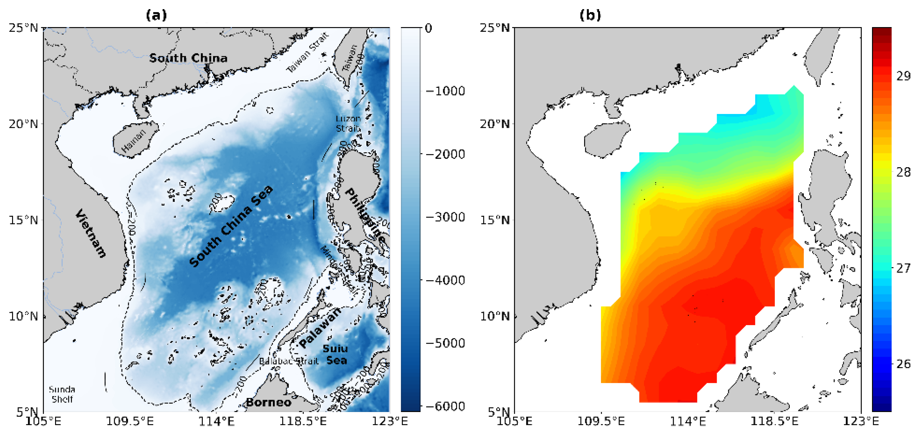
2.1. Data
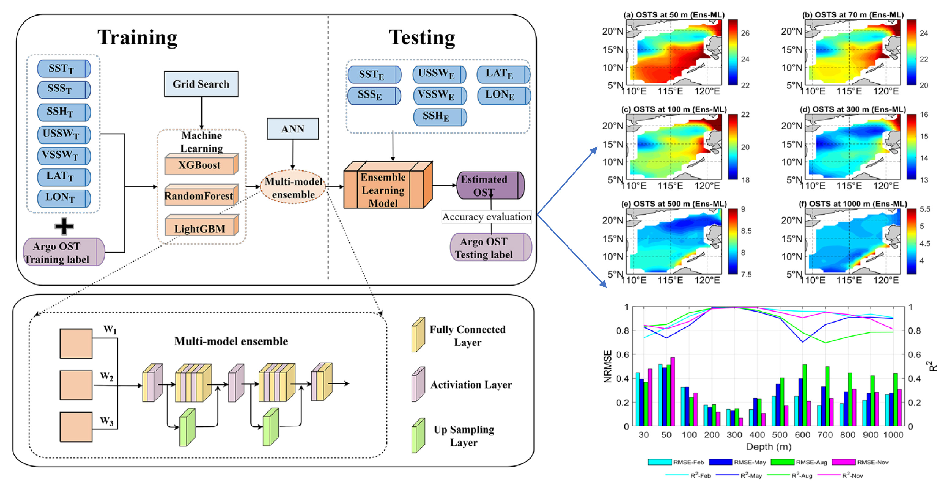
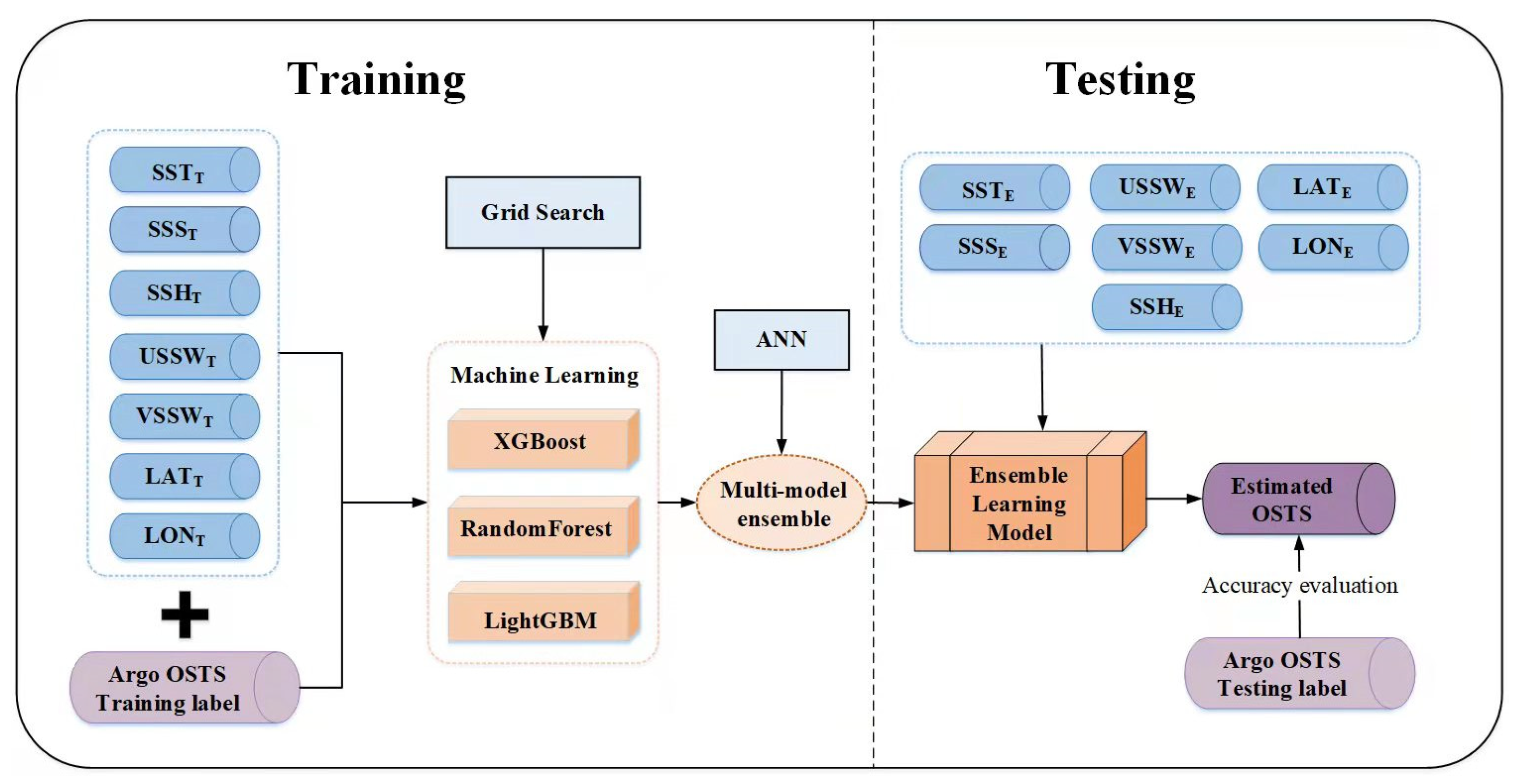
2.2. Methods
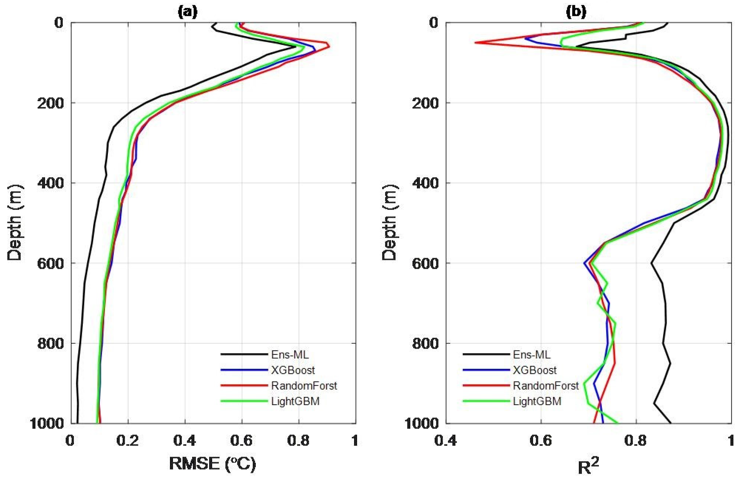
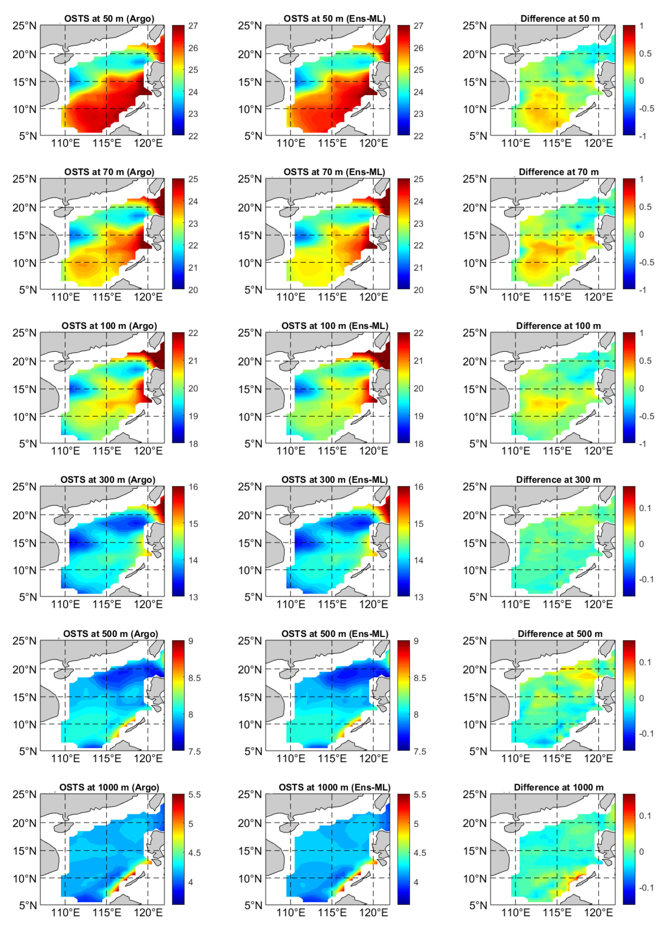
3. Results
4. Discussion and Conclusions
Author Contributions
Funding
Data Availability Statement
Acknowledgments
Conflicts of Interest
References
- Levitus, S.; Antonov, J.I.; Boyer, T.P.; Baranova, O.K.; Garcia, H.E.; Locarnini, R.A.; Mishonov, A.V.; Reagan, J.R.; Seidov, D.; Yarosh, E.S.; et al. World ocean heat content and thermosteric sea level change (0–2000 m), 1955–2010. Geophys. Res. Lett. 2012, 39, L10603. [Google Scholar] [CrossRef] [Green Version]
- Abraham, J.P.; Baringer, M.; Bindoff, N.; Boyer, T.; Cheng, L.; Church, J.A.; Conroy, J.L.; Domingues, C.M.; Fasullo, J.; Gilson, J.; et al. A review of global ocean temperature observations: Implications for ocean heat content estimates and climate change. Rev. Geophys. 2013, 51, 450–483. [Google Scholar] [CrossRef]
- Pearce, A.F.; Feng, M. The rise and fall of the “marine heat wave” off Western Australia during the summer of 2010/2011. J. Mar. Syst. 2013, 111–112, 139–156. [Google Scholar] [CrossRef]
- Oliver, E.C.J.; Donat, M.G.; Burrows, M.T.; Moore, P.J.; Smale, D.A.; Alexander, L.V.; Benthuysen, J.A.; Feng, M.; Gupta, A.S.; Hobday, A.J.; et al. Longer and more frequent marine heatwaves over the past century. Nat. Commun. 2018, 9, 1324. [Google Scholar] [CrossRef]
- Du, Y.; Zhang, Y.; Zhang, L.; Tozuka, T.; Ng, B.; Cai, W. Thermocline Warming Induced Extreme Indian Ocean Dipole in 2019. Geophys. Res. Lett. 2020, 47, e2020GL090079. [Google Scholar] [CrossRef]
- Wallace, J.M.; Rasmusson, E.M.; Mitchell, T.P.; Kousky, V.E.; Sarachik, E.S.; von Storch, H. On the structure and evolution of ENSO-related climate variability in the tropical Pacific: Lessons from TOGA. J. Geophys. Res. Earth Surf. 1998, 103, 14241–14259. [Google Scholar] [CrossRef]
- Planton, Y.Y.; Vialard, J.; Guilyardi, E.; Lengaigne, M.; McPhaden, M.J. The asymmetric influence of ocean heat content on ENSO predictability in the CNRM-CM5 coupled general circulation model. J. Clim. 2021, 34, 5775–5793. [Google Scholar] [CrossRef]
- Sprintall, J.; Tomczak, M. On the formation of central water and thermocline ventilation in the southern hemisphere. Deep Sea Res. Part I: Oceanogr. Res. Pap. 1993, 40, 827–848. [Google Scholar] [CrossRef]
- Qi, J.; Qu, T.; Yin, B.; Chi, J. Variability of the South Pacific Western Subtropical Mode Water and Its Relationship with ENSO During the Argo Period. J. Geophys. Res. Oceans 2020, 125, e2020JC016134. [Google Scholar] [CrossRef]
- Qu, T. Upper-layer circulation in the South China Sea. J. Phys. Oceanogr. 2000, 30, 1450–1460. [Google Scholar] [CrossRef]
- Qu, T.; Kim, Y.Y.; Yaremchuk, M.; Tozuka, T.; Ishida, A.; Yamagata, T. Can Luzon Strait transport play a role in conveying the impact of ENSO to the South China Sea? J. Clim. 2004, 17, 3644–3657. [Google Scholar] [CrossRef]
- Wang, G.; Xie, S.-P.; Qu, T.; Huang, R.X. Deep South China Sea circulation. Geophys. Res. Lett. 2011, 38, L05601. [Google Scholar] [CrossRef] [Green Version]
- Qi, J.; Du, Y.; Chi, J.; Yi, D.L.; Li, D.; Yin, B. Impacts of El Niño on the South China Sea surface salinity as seen from satellites. Environ. Res. Lett. 2022, 17, 054040. [Google Scholar] [CrossRef]
- Qu, T. Role of ocean dynamics in determining the mean seasonal cycle of the South China Sea surface temperature. J. Geophys. Res. Earth Surf. 2001, 106, 6943–6955. [Google Scholar] [CrossRef]
- Wang, A.; Du, Y.; Peng, S.; Liu, K.; Huang, R.X. Deep water characteristics and circulation in the South China Sea. Deep Sea Res. Part I Oceanogr. Res. Pap. 2018, 134, 55–63. [Google Scholar] [CrossRef]
- Qu, T.; Song, Y.T.; Yamagata, T. An introduction to the South China Sea throughflow: Its dynamics, variability, and application for climate. Dyn. Atmos. Oceans 2009, 47, 3–14. [Google Scholar] [CrossRef]
- Wang, D.; Wang, Q.; Cai, S.; Shang, X.; Peng, S.; Shu, Y.; Xiao, J.; Xie, X.; Zhang, Z.; Liu, Z.; et al. Advances in research of the mid-deep South China Sea circulation. Sci. China Earth Sci. 2019, 62, 1992–2004. [Google Scholar] [CrossRef]
- Yao, Y.; Wang, C. Variations in Summer Marine Heatwaves in the South China Sea. J. Geophys. Res. Oceans 2021, 126, e2021JC017792. [Google Scholar] [CrossRef]
- Chen, J.-M.; Li, T.; Shih, C.-F. Fall Persistence Barrier of Sea Surface Temperature in the South China Sea Associated with ENSO. J. Clim. 2007, 20, 158–172. [Google Scholar] [CrossRef]
- Wu, C.-R.; Shaw, P.-T.; Chao, S.-Y. Assimilating altimetric data into a South China Sea model. J. Geophys. Res. Earth Surf. 1999, 104, 29987–30005. [Google Scholar] [CrossRef] [Green Version]
- Xie, J.; Counillon, F.; Zhu, J.; Bertino, L. An eddy resolving tidal-driven model of the South China Sea assimilating along-track SLA data using the EnOI. Ocean Sci. 2011, 7, 609–627. [Google Scholar] [CrossRef] [Green Version]
- Cornillon, P.; Stramma, L.; Price, J.F. Satellite measurements of sea surface cooling during hurricane Gloria. Nature 1987, 326, 373–375. [Google Scholar] [CrossRef] [Green Version]
- Carnes, M.R.; Teague, W.J.; Mitchell, J.L. Inference of Subsurface Thermohaline Structure from Fields Measurable by Satellite. J. Atmos. Ocean. Technol. 1994, 11, 551–566. [Google Scholar] [CrossRef] [Green Version]
- Ali, M.M.; Swain, D.; Weller, R.A. Estimation of ocean subsurface thermal structure from surface parameters: A neural network approach. Geophys. Res. Lett. 2004, 31, L20308. [Google Scholar] [CrossRef] [Green Version]
- Buckingham, C.E.; Cornillon, P.C.; Schloesser, F.; Obenour, K.M. Global observations of quasi-zonal bands in microwave sea surface temperature. J. Geophys. Res. Oceans 2014, 119, 4840–4866. [Google Scholar] [CrossRef] [Green Version]
- Su, H.; Li, W.; Yan, X.-H. Retrieving Temperature Anomaly in the Global Subsurface and Deeper Ocean from Satellite Observations. J. Geophys. Res. Oceans 2018, 123, 399–410. [Google Scholar] [CrossRef]
- Mollo-Christensen, E.; Cornillon, P.; Mascarenhas, A.D.S. Method for Estimation of Ocean Current Velocity from Satellite Images. Science 1981, 212, 661–662. [Google Scholar] [CrossRef] [PubMed]
- Chu, P.C.; Fan, C.; Liu, W.T. Determination of Vertical Thermal Structure from Sea Surface Temperature. J. Atmospheric Ocean. Technol. 2000, 17, 971–979. [Google Scholar] [CrossRef] [Green Version]
- Cornillon, P.; Park, K.-A. Warm core ring velocities inferred from NSCAT. Geophys. Res. Lett. 2001, 28, 575–578. [Google Scholar] [CrossRef]
- Osychny, V.; Cornillon, P. Properties of Rossby Waves in the North Atlantic Estimated from Satellite Data. J. Phys. Oceanogr. 2004, 34, 61–76. [Google Scholar] [CrossRef] [Green Version]
- Cheng, H.; Sun, L.; Li, J. Neural Network Approach to Retrieving Ocean Subsurface Temperatures from Surface Parameters Observed by Satellites. Water 2021, 13, 388. [Google Scholar] [CrossRef]
- Willis, J.K.; Roemmich, D.; Cornuelle, B. Combining altimetric height with broadscale profile data to estimate steric height, heat storage, subsurface temperature, and sea-surface temperature variability. J. Geophys. Res. Earth Surf. 2003, 108, 3292. [Google Scholar] [CrossRef] [Green Version]
- Guinehut, S.; Dhomps, A.-L.; Larnicol, G.; Le Traon, P.-Y. High resolution 3-D temperature and salinity fields derived from in situ and satellite observations. Ocean Sci. 2012, 8, 845–857. [Google Scholar] [CrossRef] [Green Version]
- Meijers, A.J.S.; Bindoff, N.; Rintoul, S. Estimating the Four-Dimensional Structure of the Southern Ocean Using Satellite Altimetry. J. Atmospheric Ocean. Technol. 2011, 28, 548–568. [Google Scholar] [CrossRef]
- Wu, X.; Yan, X.-H.; Jo, Y.-H.; Liu, W.T. Estimation of Subsurface Temperature Anomaly in the North Atlantic Using a Self-Organizing Map Neural Network. J. Atmospheric Ocean. Technol. 2012, 29, 1675–1688. [Google Scholar] [CrossRef]
- Charantonis, A.; Badran, F.; Thiria, S. Retrieving the evolution of vertical profiles of Chlorophyll-a from satellite observations using Hidden Markov Models and Self-Organizing Topological Maps. Remote Sens. Environ. 2015, 163, 229–239. [Google Scholar] [CrossRef]
- Khedouri, E.; Szczechowski, C.; Cheney, R. Potential Oceanographic Applications of Satellite Altimetry for Inferring Subsurface Thermal Structure. In Proceedings of the OCEANS’83, San Francisco, CA, USA, 29 August–1 September 1983; pp. 274–280. [Google Scholar] [CrossRef] [Green Version]
- DeWitt, P. Model decomposition of the monthly Gulf steam/Kuroshio temperature fields. NOO Tech. Rep. 1987, 298. [Google Scholar]
- Watts, D.R.; Sun, C.; Rintoul, S. A two-dimensional gravest empirical mode determined from hydrographic observations in the Subantarctic Front. J. Phys. Oceanogr. 2001, 31, 2186–2209. [Google Scholar] [CrossRef]
- Su, H.; Huang, L.; Li, W.; Yang, X.; Yan, X. Retrieving Ocean Subsurface Temperature Using a Satellite-Based Geographically Weighted Regression Model. J. Geophys. Res. Oceans 2018, 123, 5180–5193. [Google Scholar] [CrossRef]
- Yu, F.; Zhang, X.; Chen, X.; Chen, G. Altimetry-derived ocean thermal structure reconstruction for the Bay of Bengal cyclone season. Ocean Dyn. 2020, 70, 1449–1459. [Google Scholar] [CrossRef]
- Prochaska, J.; Cornillon, P.; Reiman, D. Deep Learning of Sea Surface Temperature Patterns to Identify Ocean Extremes. Remote Sens. 2021, 13, 744. [Google Scholar] [CrossRef]
- Chen, C.; Yang, K.; Ma, Y.; Wang, Y. Reconstructing the Subsurface Temperature Field by Using Sea Surface Data Through Self-Organizing Map Method. IEEE Geosci. Remote Sens. Lett. 2018, 15, 1812–1816. [Google Scholar] [CrossRef]
- Su, H.; Wu, X.; Yan, X.-H.; Kidwell, A. Estimation of subsurface temperature anomaly in the Indian Ocean during recent global surface warming hiatus from satellite measurements: A support vector machine approach. Remote Sens. Environ. 2015, 160, 63–71. [Google Scholar] [CrossRef]
- Li, W.E.; Su, H.; Wang, X.; Yan, X. Estimation of global subsurface temperature anomaly based on multisource satellite obser-vations. J. Remote. Sens. 2017, 21, 881–891. [Google Scholar]
- Su, H.; Yang, X.; Lu, W.; Yan, X.-H. Estimating Subsurface Thermohaline Structure of the Global Ocean Using Surface Remote Sensing Observations. Remote Sens. 2019, 11, 1598. [Google Scholar] [CrossRef] [Green Version]
- Su, H.; Wang, A.; Zhang, T.; Qin, T.; Du, X.; Yan, X.-H. Super-resolution of subsurface temperature field from remote sensing observations based on machine learning. Int. J. Appl. Earth Obs. Geoinf. 2021, 102, 102440. [Google Scholar] [CrossRef]
- Han, M.; Feng, Y.; Zhao, X.; Sun, C.; Hong, F.; Liu, C. A Convolutional Neural Network Using Surface Data to Predict Subsurface Temperatures in the Pacific Ocean. IEEE Access 2019, 7, 172816–172829. [Google Scholar] [CrossRef]
- Lu, W.; Su, H.; Yang, X.; Yan, X.-H. Subsurface temperature estimation from remote sensing data using a clustering-neural network method. Remote Sens. Environ. 2019, 229, 213–222. [Google Scholar] [CrossRef]
- Nardelli, B.B. A Deep Learning Network to Retrieve Ocean Hydrographic Profiles from Combined Satellite and In Situ Measurements. Remote Sens. 2020, 12, 3151. [Google Scholar] [CrossRef]
- Meng, L.; Yan, C.; Zhuang, W.; Zhang, W.; Geng, X.; Yan, X.-H. Reconstructing High-Resolution Ocean Subsurface and Interior Temperature and Salinity Anomalies from Satellite Observations. IEEE Trans. Geosci. Remote Sens. 2021, 60, 1–14. [Google Scholar] [CrossRef]
- Xiao, C.; Chen, N.; Hu, C.; Wang, K.; Gong, J.; Chen, Z. Short and mid-term sea surface temperature prediction using time-series satellite data and LSTM-AdaBoost combination approach. Remote Sens. Environ. 2019, 233, 111358. [Google Scholar] [CrossRef]
- Wolff, S.; O’Donncha, F.; Chen, B. Statistical and machine learning ensemble modelling to forecast sea surface temperature. J. Mar. Syst. 2020, 208, 103347. [Google Scholar] [CrossRef]
- Gracia, S.; Olivito, J.; Resano, J.; Martin-Del-Brio, B.; de Alfonso, M.; Álvarez, E. Improving accuracy on wave height estimation through machine learning techniques. Ocean Eng. 2021, 236, 108699. [Google Scholar] [CrossRef]
- Reynolds, R.W.; Rayner, N.A.; Smith, T.M.; Stokes, D.C.; Wang, W. An improved in situ and satellite SST analysis for climate. J. Clim. 2002, 15, 1609–1625. [Google Scholar] [CrossRef]
- Boutin, J.; Vergely, J.; Marchand, S.; D’Amico, F.; Hasson, A.; Kolodziejczyk, N.; Reul, N.; Reverdin, G.; Vialard, J. New SMOS Sea Surface Salinity with reduced systematic errors and improved variability. Remote Sens. Environ. 2018, 214, 115–134. [Google Scholar] [CrossRef] [Green Version]
- Hauser, D.; Tourain, C.; Hermozo, L.; Alraddawi, D.; Aouf, L.; Chapron, B.; Dalphinet, A.; Delaye, L.; Dalila, M.; Dormy, E.; et al. New Observations from the SWIM Radar On-Board CFOSAT: Instrument Validation and Ocean Wave Measurement Assessment. IEEE Trans. Geosci. Remote Sens. 2020, 59, 5–26. [Google Scholar] [CrossRef]
- Atlas, R.; Hoffman, R.; Ardizzone, J.; Leidner, S.M.; Jusem, J.C.; Smith, D.K.; Gombos, D. A Cross-calibrated, Multiplatform Ocean Surface Wind Velocity Product for Meteorological and Oceanographic Applications. Bull. Am. Meteorol. Soc. 2011, 92, 157–174. [Google Scholar] [CrossRef]
- Roemmich, D.; Gilson, J. The 2004–2008 mean and annual cycle of temperature, salinity, and steric height in the global ocean from the Argo Program. Prog. Oceanogr. 2009, 82, 81–100. [Google Scholar] [CrossRef]
- Rajabi-Kiasari, S.; Hasanlou, M. An efficient model for the prediction of SMAP sea surface salinity using machine learning approaches in the Persian Gulf. Int. J. Remote Sens. 2019, 41, 3221–3242. [Google Scholar] [CrossRef]
- Liu, Q.; Jia, Y.; Liu, P.; Wang, Q.; Chu, P.C. Seasonal and intraseasonal thermocline variability in the central south China Sea. Geophys. Res. Lett. 2001, 28, 4467–4470. [Google Scholar] [CrossRef] [Green Version]
- Wang, Y.; Castelao, R.M.; Yuan, Y. Seasonal variability of alongshore winds and sea surface temperature fronts in Eastern Boundary Current Systems. J. Geophys. Res. Oceans 2015, 120, 2385–2400. [Google Scholar] [CrossRef]
- Wang, Y.; Castelao, R.M. Variability in the coupling between sea surface temperature and wind stress in the global coastal ocean. Cont. Shelf Res. 2016, 125, 88–96. [Google Scholar] [CrossRef]
- Wang, Y.; Liu, J.; Liu, H.; Lin, P.; Yuan, Y.; Chai, F. Seasonal and Interannual Variability in the Sea Surface Temperature Front in the Eastern Pacific Ocean. J. Geophys. Res. Oceans 2021, 126, e2020JC016356. [Google Scholar] [CrossRef]
- Zheng, G.; Li, X.; Zhang, R.-H.; Liu, B. Purely satellite data–driven deep learning forecast of complicated tropical instability waves. Sci. Adv. 2020, 6, eaba1482. [Google Scholar] [CrossRef]


| Index | Contents | |||
|---|---|---|---|---|
| Study Area | South China Sea | 105–122°E, 5–23°N | ||
| Data | SST | 2010–2019 | NOAA (OISST) | input |
| SSS | 2010–2019 | SMOS | ||
| SSH | 2010–2019 | AVISO | ||
| SSW (USSW, VSSW) | 2010–2019 | CCMP | ||
| OSTS | 2010–2019 | RG-Argo | output | |
| 3D temperature field | Temporal and spatial resolution | monthly | 0.5° × 0.5° | |
| Vertical layers | 2.5–1000 m | 44 layers | ||
| Model | Parameters |
|---|---|
| XGBoost | learning_rate = 0.3, n_estimators = 60, max_depth = 6, min_child_weight = 1, colsample_bytree = 1, colsample_bylevel = 1, subsample = 0.8, reg_lambda = 100 |
| RandomForest | n_estimators = 150, max_depth = 21, min_samples_split = 70, min_samples_leaf = 3, max_features = 5, random_state = 10 |
| LightGBM | num_leaves = 55, learning_rate = 0.01, n_estimators = 1000, max_depth = 8, min_child_samples = 20, feature_fraction = 0.8 |
| ANN | number of neural network layers = 4, Residual layers = 2, learning rate = 0.002, batch_size = 1024 |
| OSTS Estimation Models | RMSE | R2 |
|---|---|---|
| Ens-ML | 0.31 | 0.89 |
| XGBoost | 0.39 | 0.83 |
| RandomForest | 0.40 | 0.83 |
| LightGBM | 0.37 | 0.84 |
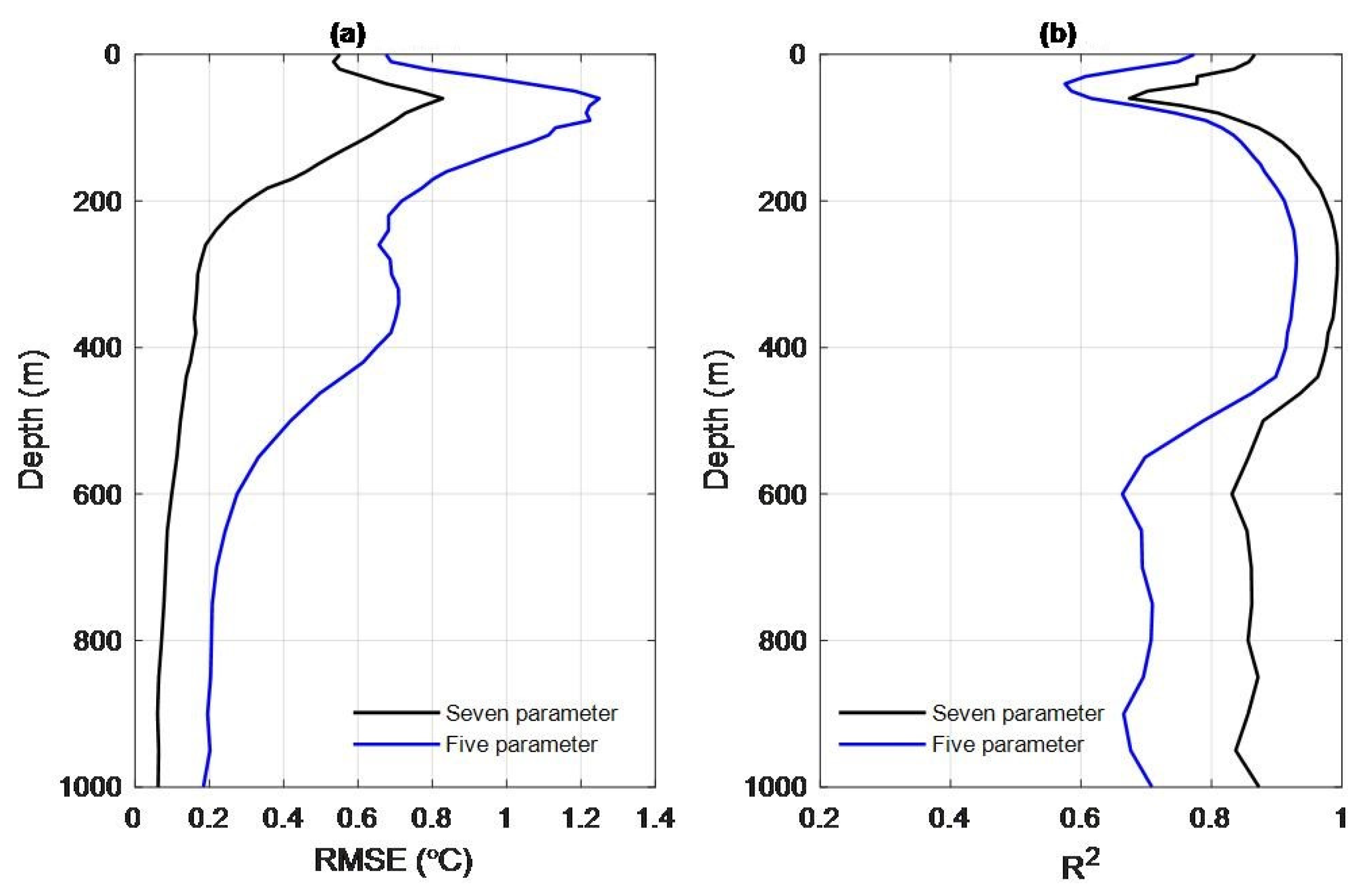
| Experiments | Training Methods |
|---|---|
| Case 1 (five parameters) | OSTS = Ensemble (SST, SSS, SSH, USSW, VSSW) |
| Case 2 (seven parameters) | OSTS = Ensemble (SST, SSS, SSH, USSW, VSSW, LON, LAT) |
| Depth (m) | RMSE | R2 |
|---|---|---|
| 2.5 | 0.51 | 0.86 |
| 10 | 0.49 | 0.85 |
| 20 | 0.51 | 0.83 |
| 30 | 0.57 | 0.77 |
| 50 | 0.72 | 0.72 |
| 70 | 0.73 | 0.75 |
| 100 | 0.62 | 0.87 |
| 150 | 0.45 | 0.94 |
| 200 | 0.26 | 0.97 |
| 300 | 0.12 | 0.99 |
| 400 | 0.11 | 0.97 |
| 500 | 0.08 | 0.87 |
| 600 | 0.05 | 0.83 |
| 700 | 0.04 | 0.86 |
| 800 | 0.03 | 0.85 |
| 900 | 0.02 | 0.85 |
| 1000 | 0.02 | 0.87 |
Publisher’s Note: MDPI stays neutral with regard to jurisdictional claims in published maps and institutional affiliations. |
© 2022 by the authors. Licensee MDPI, Basel, Switzerland. This article is an open access article distributed under the terms and conditions of the Creative Commons Attribution (CC BY) license (https://creativecommons.org/licenses/by/4.0/).
Share and Cite
Qi, J.; Liu, C.; Chi, J.; Li, D.; Gao, L.; Yin, B. An Ensemble-Based Machine Learning Model for Estimation of Subsurface Thermal Structure in the South China Sea. Remote Sens. 2022, 14, 3207. https://doi.org/10.3390/rs14133207
Qi J, Liu C, Chi J, Li D, Gao L, Yin B. An Ensemble-Based Machine Learning Model for Estimation of Subsurface Thermal Structure in the South China Sea. Remote Sensing. 2022; 14(13):3207. https://doi.org/10.3390/rs14133207
Chicago/Turabian StyleQi, Jifeng, Chuanyu Liu, Jianwei Chi, Delei Li, Le Gao, and Baoshu Yin. 2022. "An Ensemble-Based Machine Learning Model for Estimation of Subsurface Thermal Structure in the South China Sea" Remote Sensing 14, no. 13: 3207. https://doi.org/10.3390/rs14133207