1. Introduction
The Special Sensor Microwave Imager/Sounder instrument (SSMIS) onboard the US Air Force Defense Meteorological Satellite Program (DMSP) polar-orbiting satellite F16, launched on 18 October 2003, was the successor and combination of the Special Sensor Microwave/Imagers (SSM/I), the Special Sensor Microwave/Temperature Sounder (SSM/T), and the Special Sensor Microwave/Water Vapor Sounder (SSM/T2) onboard the F10–15. As a conical scanning radiometer with a constant 45° scan angle, the SSMIS’s 24 channels, whose central frequencies range from 19 to 183 GHz, are primarily designed to enhance remote-sensing capabilities of the land surface, ocean surface wind speed, cloud liquid, and rain rate (channels 12–18), measure the atmospheric radiation from the surface to about 30 hPa (channels 1–7), the upper troposphere (channel 24, ~12 hPa) and the mesosphere (channel 19, ~0.28 hPa), and obtain features sensitive to water vapor contents in the middle and lower troposphere (channels 8–11). SSMIS field-of-view (FOV) sizes are the same, and the distance between any two neighboring FOVs along a scan line does not vary. Therefore, weather-related structures are directly visible in global TB observations at channels 1–7, often called lower atmospheric sounding (LAS) channels. The F16 SSMIS TB observations have been available to the general public since 20 November 2005. As of now, we have more than 16 years of F16 SSMIS observations. Unfortunately, a significant data noise has occurred in F16 SSMIS TB observations since 25 April 2013. Our study analyzes these noise characteristics and develops an appropriate noise-detection algorithm for F16 SSMIS observations. Only then can we explore a unique opportunity to study the weather and climate of the atmosphere over 16 years using simultaneous measurements of imager channels, temperature-sounding channels, and humidity-sounding channels from F16 SSMIS.
Using satellite microwave observations to study the weather and climate of the atmosphere has been conducted more substantially using cross-track temperature sounders since the earliest Microwave Sounding Unit (MSU) onboard the National Oceanic and Atmospheric Administration (NOAA) polar-orbiting satellites TIROS-N, which was launched on 13 October 1978. The 4-channel MSU onboard TIROS-N, NOAA-6 to NOAA-14 was then replaced by the 15-channel Advanced Microwave Sounding Unit-A (AMSU-A) when NOAA-15 was launched on 13 May 1998. The AMSU-A onboard NOAA-15 to NOAA-19 and MetOp-A/B/C [
1,
2] was finally replaced by the Advanced Technology Microwave Sounders (ATMS) when S-NPP and NOAA-20 were launched on 28 October 2011 and 18 November 2017, respectively [
3]. The global TB observations from multiple cross-track microwave temperature sounders have more than 40 years of continuous data records [
4] that are routinely assimilated into NWP systems at nearly all operational centers and have contributed to significant improvements in global NWP forecast skills at the National Centers for Environmental Prediction (NCEP) [
5], the European Centre of Medium-Range Weather Forecasts (ECMWF) [
6,
7], and China [
8,
9]. However, as a unique feature of cross-track radiometers, the limb effect causes the structural features of weather not to be directly visible from TB observations. This finding is not the case for TB observations from the conical scanning radiometer SSMIS.
Among different weather systems, tropical cyclones (TCs) remain of great interest to research and operational forecasts [
10,
11,
12,
13]. Due to the fast-evolving nature of their structure, track, and intensity controlled by complex, dynamic physics processes and societal impacts, satellite observations have become instrumental for investigating and predicting TCs that are mostly over oceans where conventional observations are rare. Besides direct assimilation of conical scanning microwave observations [
14,
15,
16,
17], another way to fully explore the potential values of polar-orbiting satellite microwave TB observations for TC research and forecasts is to apply TC warm core, TC center position, and inner and outer rainband sizes derivable from TB observations to vortex initialization. The microwave radiance is approximately a linear function of the atmospheric temperature at frequencies <200 GHz, larger than all SSMIS and AMSU-A channel frequencies. Based on this physical consideration, TC warm-core anomalies can be retrieved based on TB observations from these microwave instruments [
18,
19,
20,
21,
22]. The assimilation of satellite microwaves retrieved TC warm-core temperatures improved 48-h forecasts of intensifications and vertical structures of all model state variables (e.g., temperature, water vapor mixing ratio, liquid water content mixing ratio, tangential and radial wind components, and vertical velocity) for Hurricane Florence (2018) and Typhoon Mangkhut (2018) [
23]. Hu and Zou [
24,
25] developed an azimuthal-spectral-analysis-based center-fixing algorithm to determine the TC center position in real-time using the TC’s axisymmetric structural information embedded in TB observations. The noise, if not detected and removed, prevents the application or reduces the accuracy of the TC warm-core retrieval and TC center positioning using SSMIS TB observations.
The conical-scanning node makes SSMIS LAS channels a potentially important data source complementing cross-track radiometers in revealing TC structures. The long-term F16 SSMIS data availability also allows an investigation into the decadal change of TCs. For these purposes, we aimed to remove the noise found in the F16 SSMIS LAS channels from 25 April 2013 onward. Our paper is organized as follows:
Section 2 briefly describes F-16 SSMIS TB observations of LAS channels.
Section 3 describes methods for analyzing and mitigating data noise. Our results are presented in
Section 4, showing temporal and latitudinal dependences of data noise in F-16 SSMIS LAS channels TB observations. Methods to avoid artificial errors induced by noise mitigation due to sharp TB variations over TC heavy rainfall areas are discussed in
Section 5. Our conclusions and future plans are provided in
Section 6.
2. Data Description
DMSP F16 is a sun-synchronous polar-orbit satellite at an altitude of approximately 833 km, circling the Earth at 14.1 revolutions per day. The SSMIS instrument onboard F16 is a conically scanning passive microwave radiometer that collects data from the aft (forward) to the nadir for a morning ascending (descending) node orbit. It measures upwelling microwave radiation from 24 channels located in a range of frequencies from 19 to 183 GHz [
26]. These 24 channels consist of the lower atmospheric sounding (LAS) channels 1–7 and 24, the environmental sensor channels 12–16, imager channels 8–11 and 17–18, and upper atmospheric sounding channels 19–23. Although only the SSMIS channels 12–18 from F16, F17, and F18 were intercalibrated to SSM/I equivalent channels to generate the so-called Fundamental Climate Data Record (FCDR) of TB data from the SSMIS sensors, the output FCDR file also contains the TB and geolocation information for all the other SSMIS channels with limited corrections and no intercalibration applied [
27]. Ten years since its launch date, TB observations of the SSMIS LAS channels from DMSP F16 were contaminated by obvious noise, preventing any possible attempts to study climate change. Our study focuses on F16 SSMIS LAS channels.
Channel characteristics for the LAS channels are shown in
Table 1. The LAS channels are located in the oxygen (O
2) band and provide measurements of upwelling microwave radiances responding to emissions and absorption due to O
2 rotational transitions. They provide information on atmospheric temperature. The eight LAS channels are designed to profile atmospheric temperature from the surface to the upper stratosphere near 12 hPa. Channel 1 is the window channel, and other LAS channels are sounding channels. A TB measurement from a particular channel quantifies a radiation amount from a vertical layer of the atmosphere centered around the altitude of the maximum weighting function (WF) shown in
Table 1. The SSMIS antenna bore-sight is designed at a 45° angle off the nadir so that the SSMIS conically scans the Earth’s surface at an incidence angle of 53°With a swath width of 1707 km. All fields-of-view (FOVs) are 27 × 18 km
2 in the along- and across-track directions. The sampling interval is the same as 12.5 × 37.5 km
2 for channels 1–7 and channel 24 in the along- and across-track directions. In 1.9 s, SSMIS can measure 60 scenes (i.e., FOVs) within a scan range of 143.2 degrees along a single scanline. Although later than MSU and much later than AMSU-A, the F16 SSMIS is the first instrument employing a conical scan geometry for temperature sounding [
28].
We obtained the F16 SSMIS data used in this study from the following website:
http://rain.atmos.colostate.edu/FCDR/data_access.html (accessed on 5 January 2022).
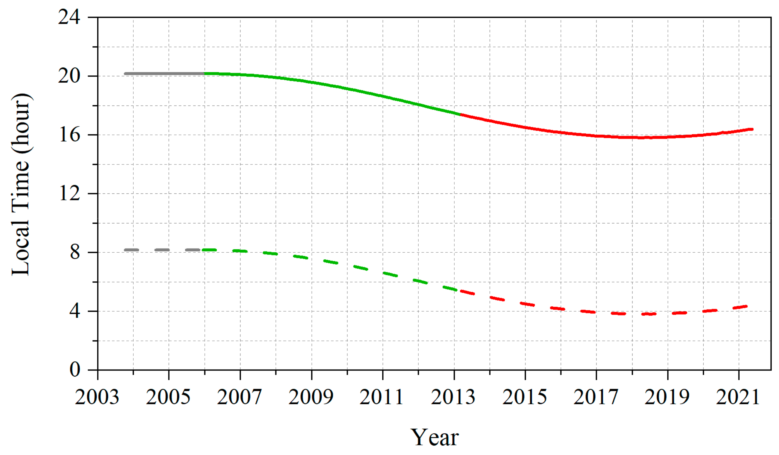
Figure 1 shows the local equator crossing time (LECT) variations of F16 from its launch to 15 June 2021, the last day of available F16 SSMIS data (
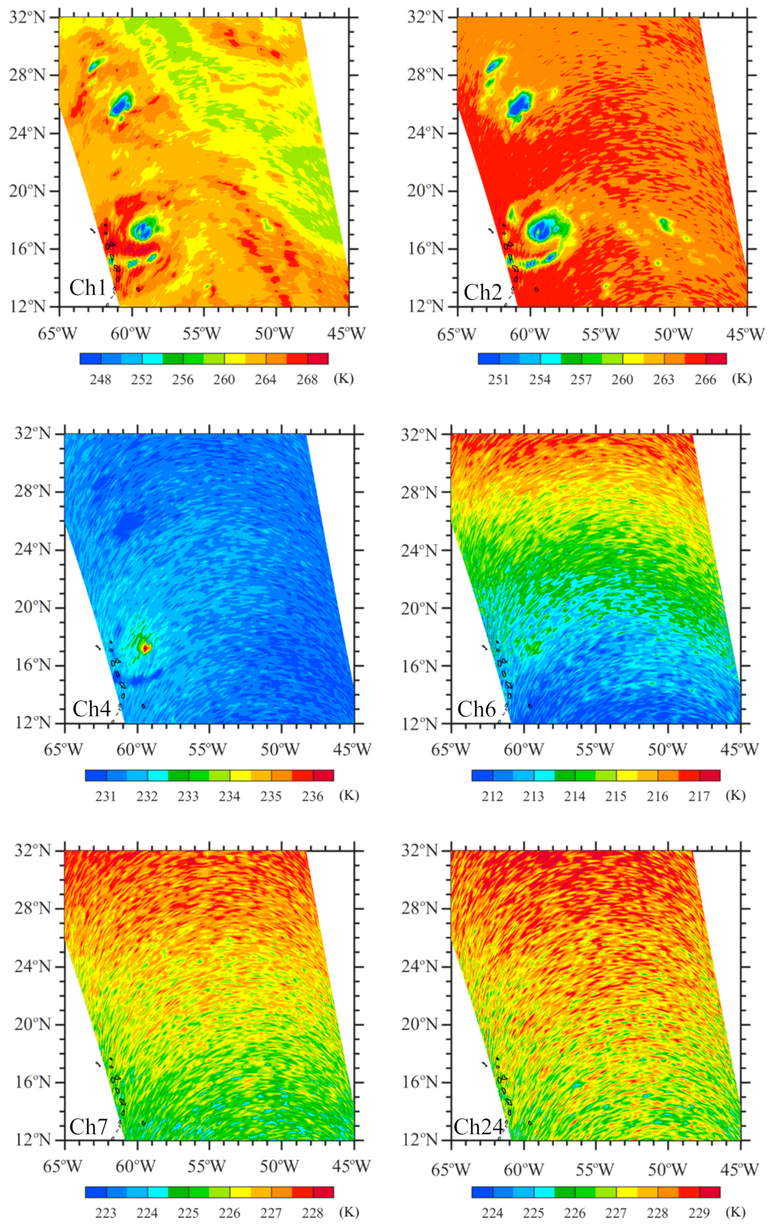
Figure 1). We found systematic noise in TB observations of F16 SSMIS LAS channels since 25 April 2013. For example,
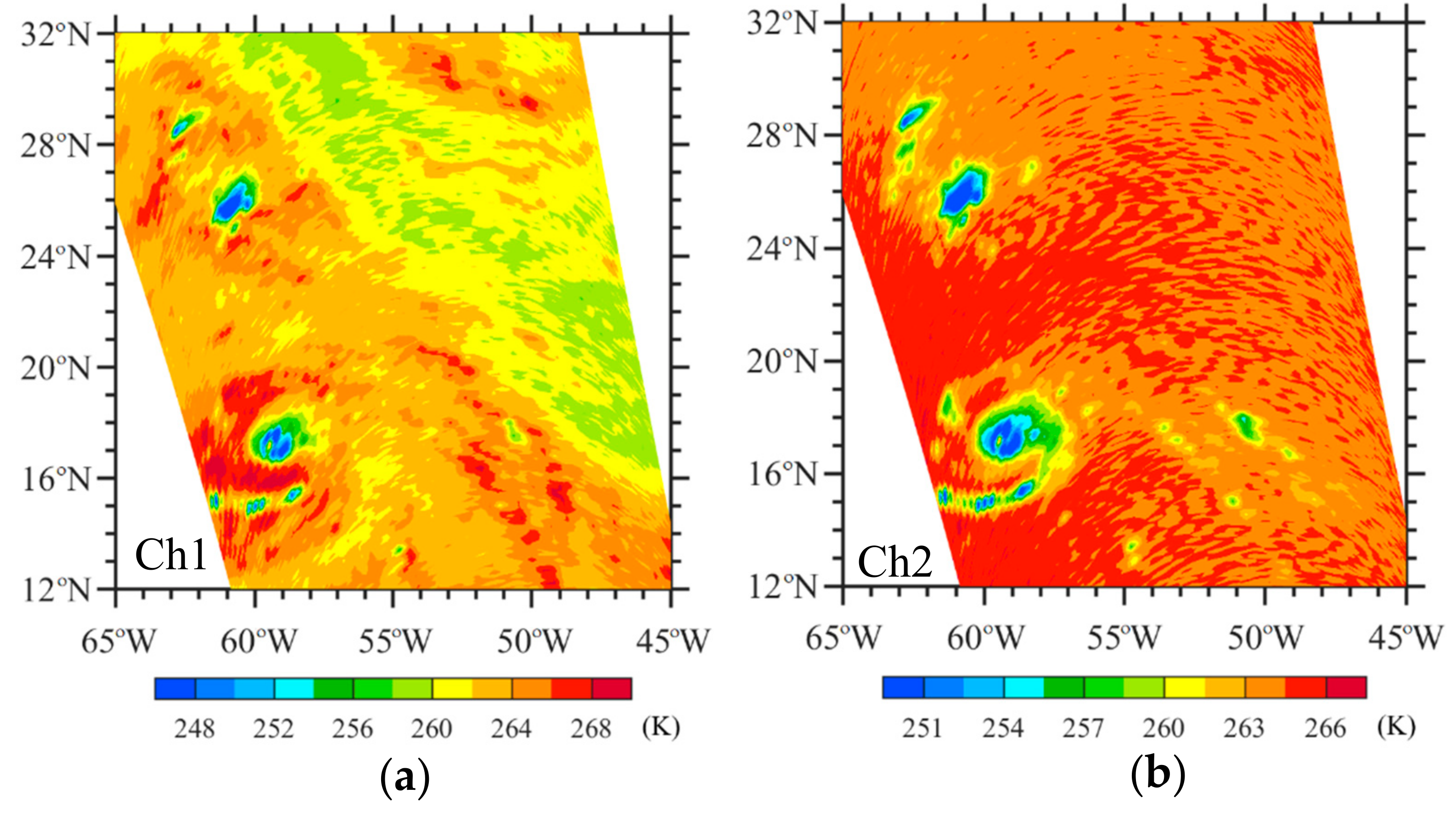
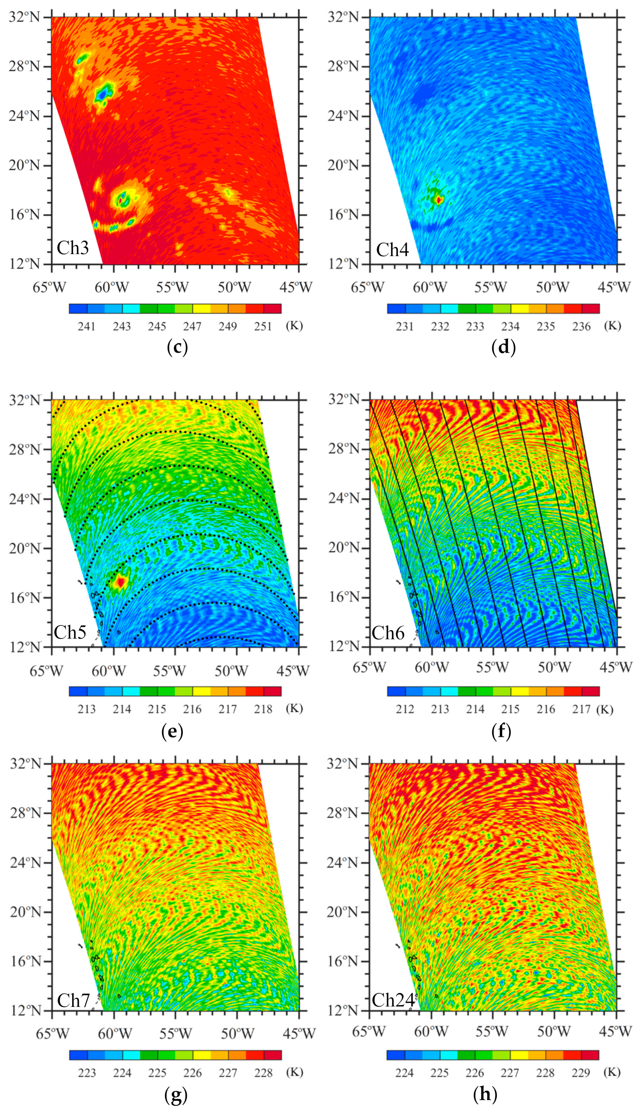
Figure 2 provides spatial distributions of TB observations at channels 1–7 and 24 over a small portion of an ascending swath on 5 September 2017. A systematic curvy noise pattern was seen in all TB observations of the LAS channels. The higher the channels’ WF peak altitudes, the clearer the noise distributions because this part of the swath went over Hurricane Irma, whose associated cloud and precipitation affected low-level TB observations more than high-level channels. The dynamic range of TB observations for channels 4–7 and 24 (~4–5 K) are much smaller than those of channels 1–3 (~10–20 K) for the part shown in
Figure 2. To search for a possible law of the curvy noise scanning pattern of the conical radiometer SSMIS, we indicated across-track distributions of 60 FOVs along several SSMIS scanlines at an interval of 25 scanlines in
Figure 2e and along-track distributions of FOVs at an interval of 5 FOVs in
Figure 2f. With this noise observation, we developed a method for mitigating TB noise in the F16 SSMIS LAS channels.
3. Method for Noise Mitigation
Using the two-dimensional (2D) discrete fast Fourier transform (FFT), we can express the TB observations over a targeted portion of swath as follows:
where
represents the TB observation at the
ith FOV and the
jth scanline (
I = 1, 2, …,
M,
j = 1, 2, …,
N);
M is the total number of FOVs along a single scanline (
M = 60);
N is the total number of scanlines (
N ≈ 300); and
is the amplitude of the 2D wave with wavenumbers
m and
n in the across- and along-track directions, respectively. The inverse Fourier transform is defined as follows:
The wavelength () in the across-track direction is calculated from the wavenumber (m) using the formula , where is equal to the across-track sampling interval of 37.5 km. Similarly, the wavelength () in the along-track direction is calculated from the wavenumber (n) using the formula , where is equal to the along-track sampling interval of 12.5 km.
In general, the TB amplitude decreases rapidly with the increasing wavenumber. If there is a sudden increase in amplitude within a range of wavenumbers
, we can remove these wave components by setting the amplitude
to zero when
for all
n. The reconstructed TB field is obtained by the inverse FFT:
The data noise is defined as . The above procedure to generate noise-mitigated TB observations () is applied to LAS channels 5–7 and 24.
In the presence of heavy precipitation, TB observations have outliers of an abnormally small value. Some of these low TB values sneak into extracted noise. We conducted an extra step to avoid the impacts of heavy precipitation-induced TB outliers of abnormally small value on noise mitigation. Specifically, we used an Empirical Mode Decomposition (EMD) developed by Huang et al. [
29] to extract the high-frequency random noise from TB observations along a scanline. The highest frequency across-track variation, called the first intrinsic mode function (IMF), is extracted from TB observations and obtained by identifying all the local maxima and minima of
(
k = 1, 2, …,
M). All the local maxima are then connected with a cubic spline as the upper envelope, and all the local minima are connected with a cubic spline as the lower envelope. The upper and lower envelopes are finally averaged to obtain the local mean, denoted as
. The 1st IMF of
(
k = 1, 2, …,
M) is defined as:
If at some FOVs (
), values of the first IMF are greater than 1.7 times the bi-weight standard deviation, these FOVs are subtracted from TB observations:
A 2D spectral analysis is conducted for the field of
. The values subtracted on the right-hand-side of (6) are added back to the noise-mitigated TB field:
The above procedure is used to generate noise-mitigated TB observations () for LAS channels 1–4. Data noise is defined as .
4. Results Characterizing a Systematic Noise in F16 SSMIS LAS TB Observations
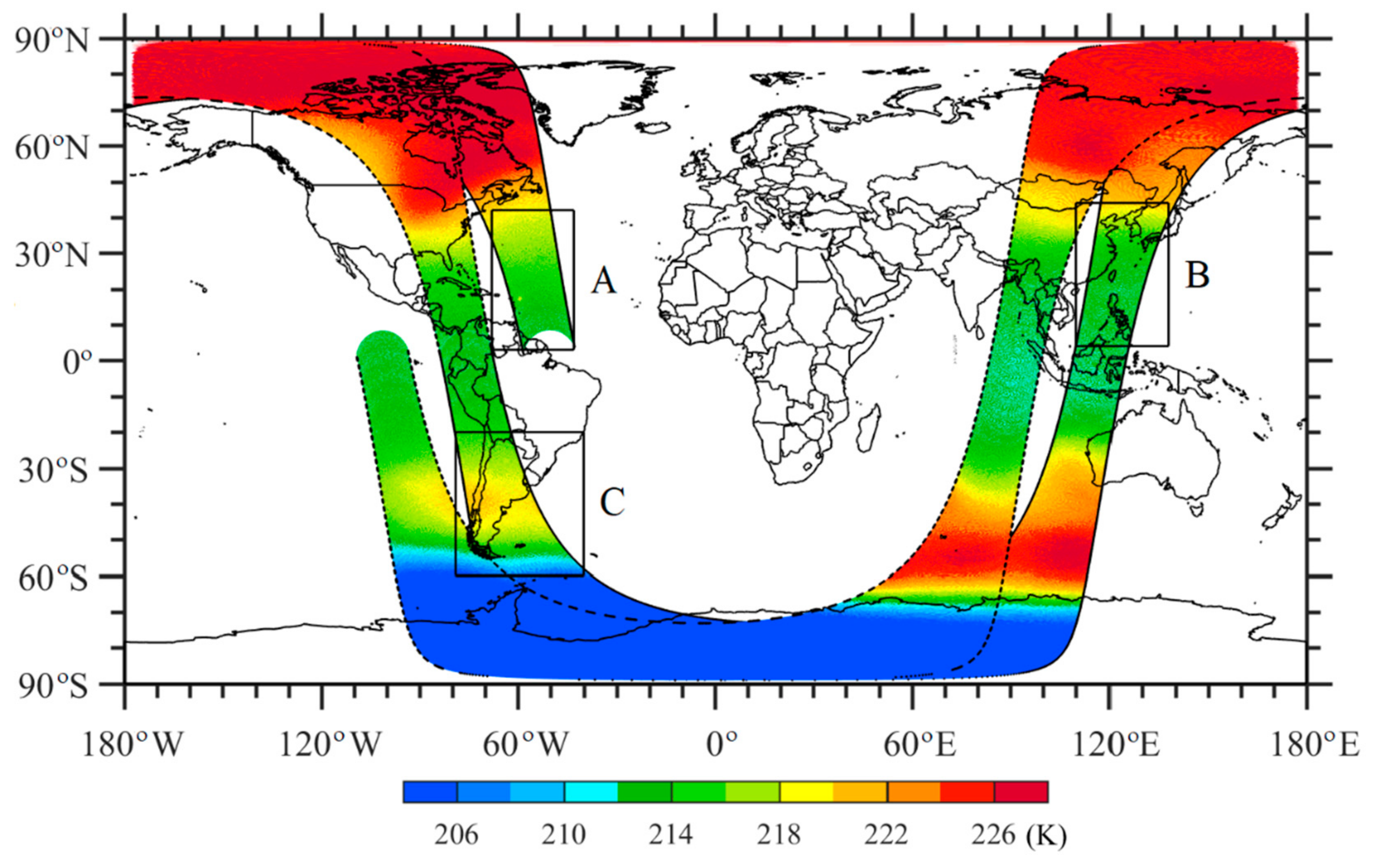
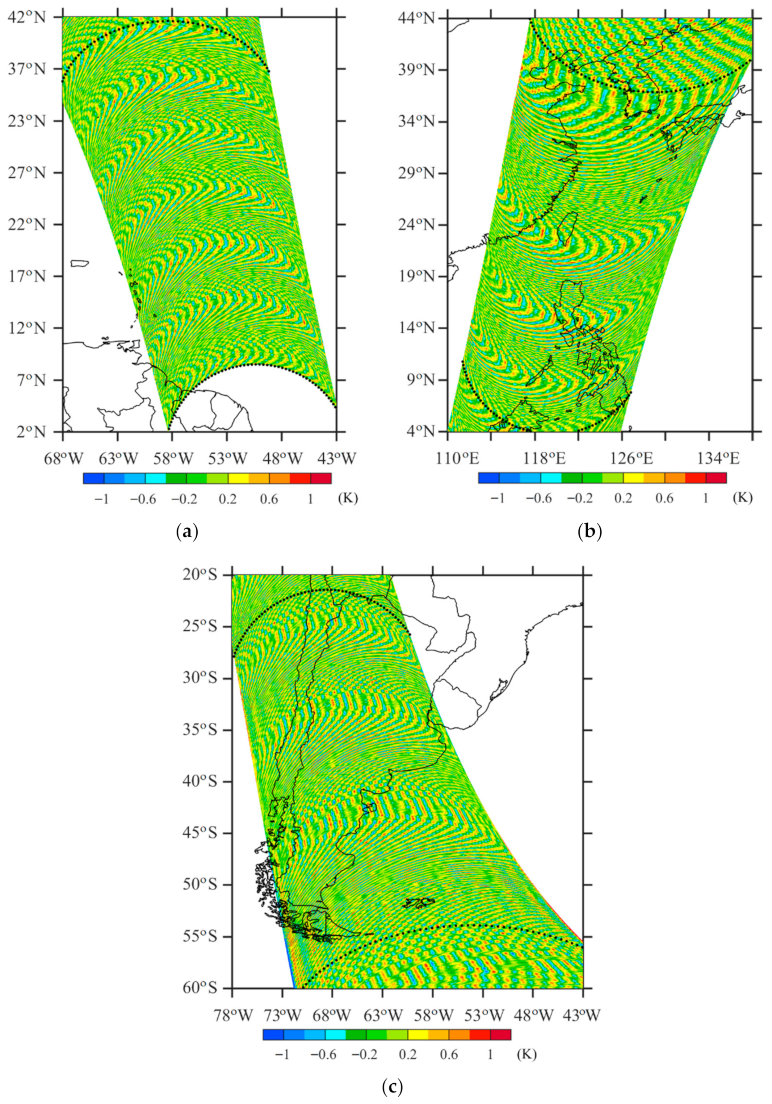
Two sequential SSMIS swaths are provided in
Figure 3, which shows TB observations from channel 5 on 5 September 2017. The observation times for the swath whose edges are indicated by solid black curves were from 1915 to 2057 UTC; those for the other swath with edges indicated by black dashed curves are from 2057 to 2238 UTC. There are orbital gaps in low latitudes. The global TB observations vary more than 20 K, characterized by a significant latitudinal distribution. The TBs near the south pole are below 206 K, and those near the north pole are above 226 K. The TBs near the equator are around 214 K. It is difficult to see any noise structures in
Figure 3 with more than a 20 K range of TB variations and 7 K color interval.
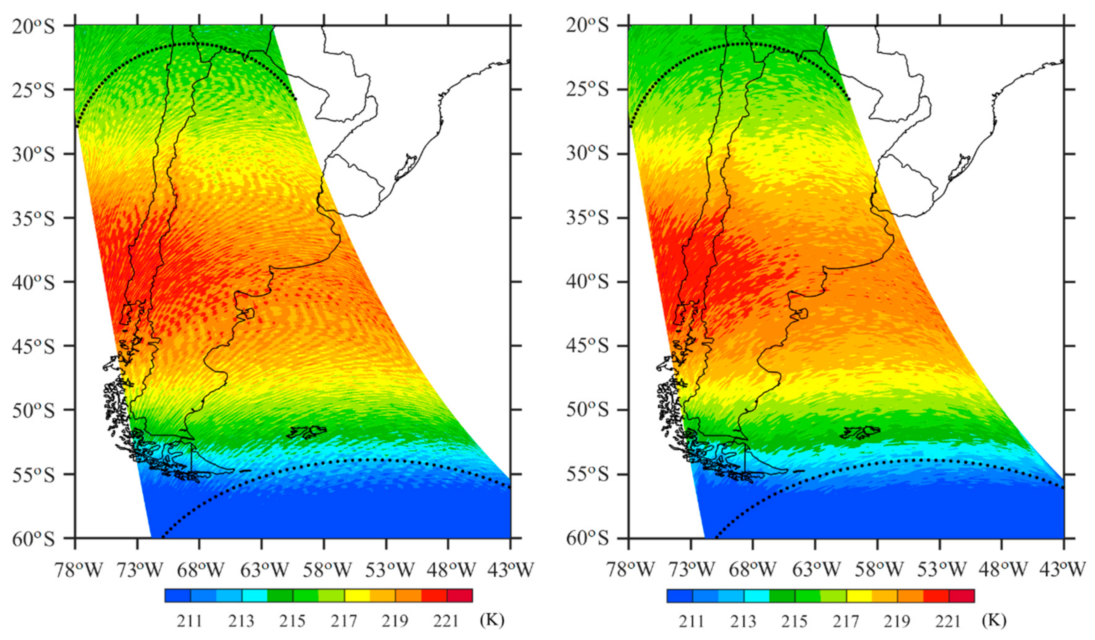
We arbitrarily chose the following three areas of the first swath in
Figure 3 for a more detailed analysis. Areas A and C are two portions at the ascending node over the western Northern and Southern Hemispheres, respectively. Area B is at the descending node over the eastern Northern Hemisphere. All three areas contain 300 scanlines. The dynamic range of channel 5 TB observations over the three local areas A, B, and C is reduced to about 5–10 K (
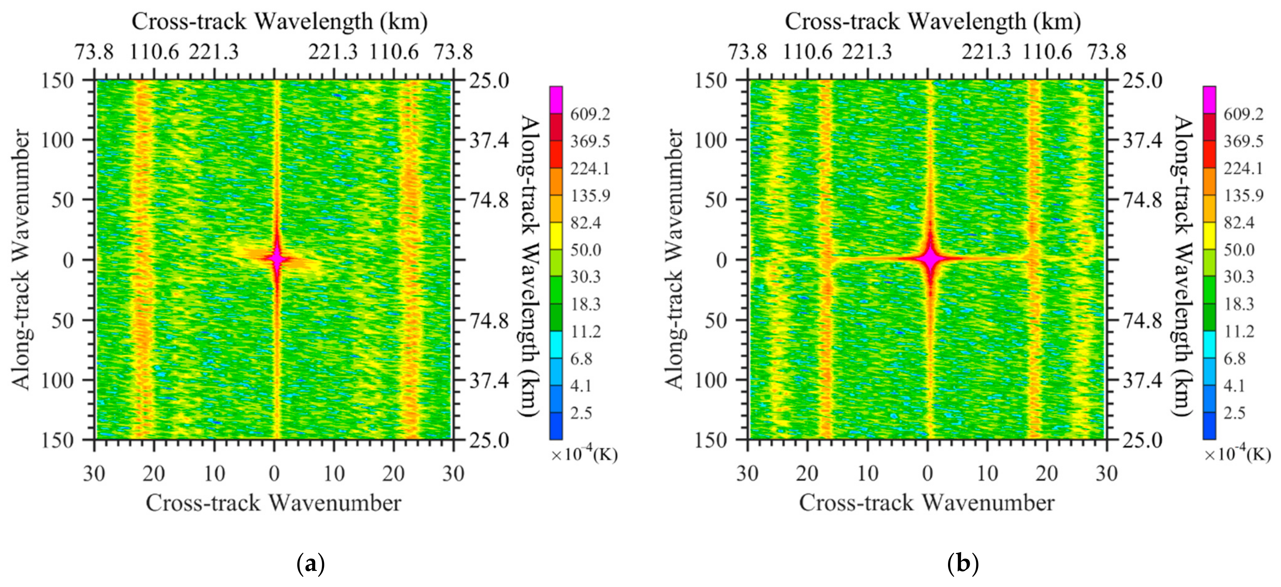
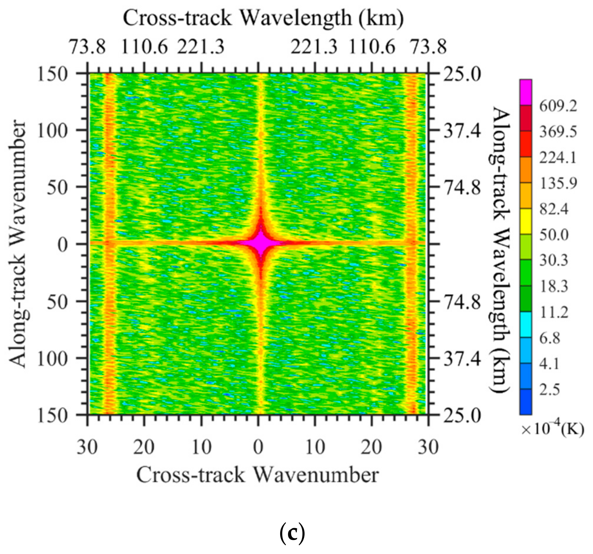
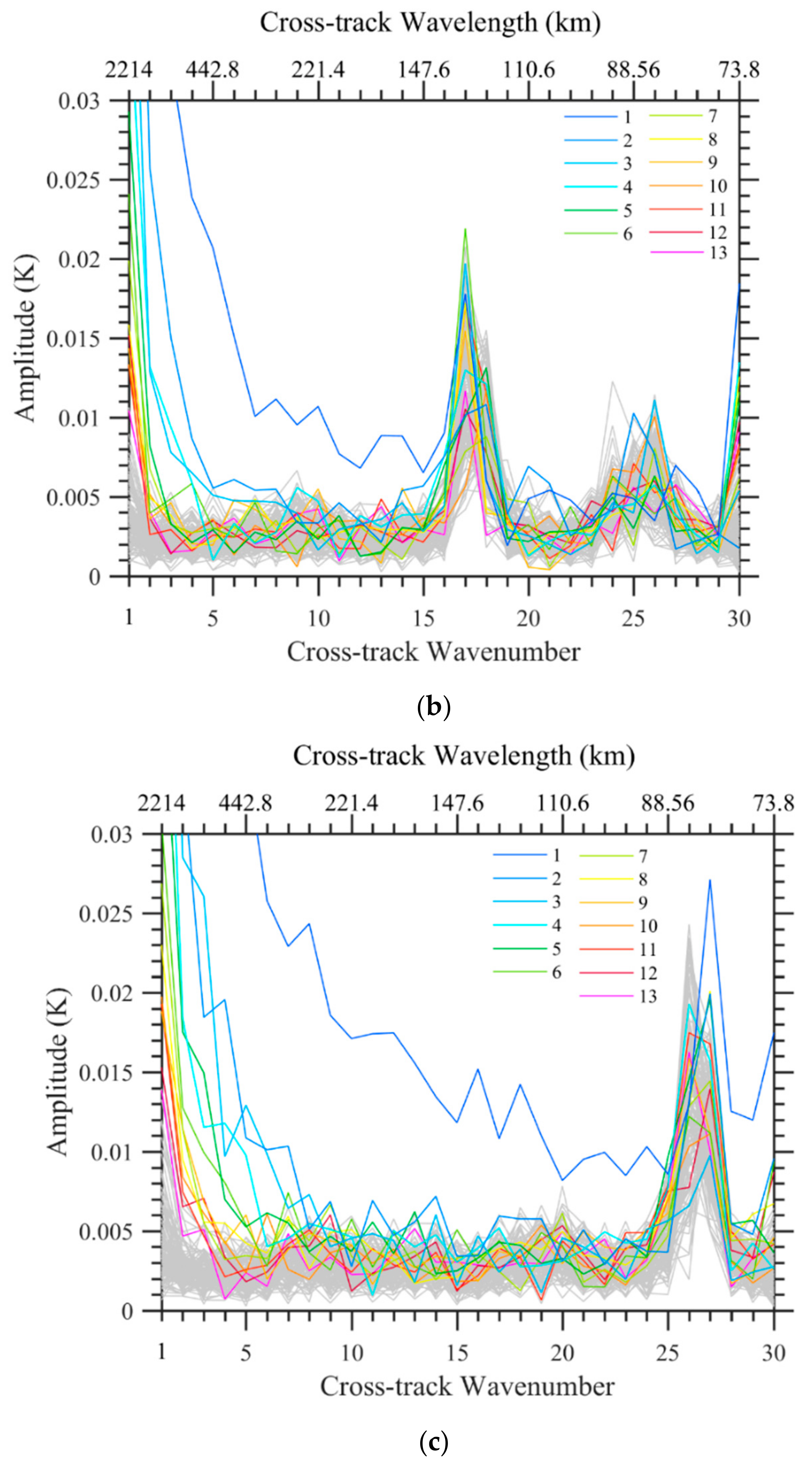
Figure 4), and a systematic noise pattern of a curvy shape becomes visible in the distributions of TB observations. A 2D spectral analysis described in
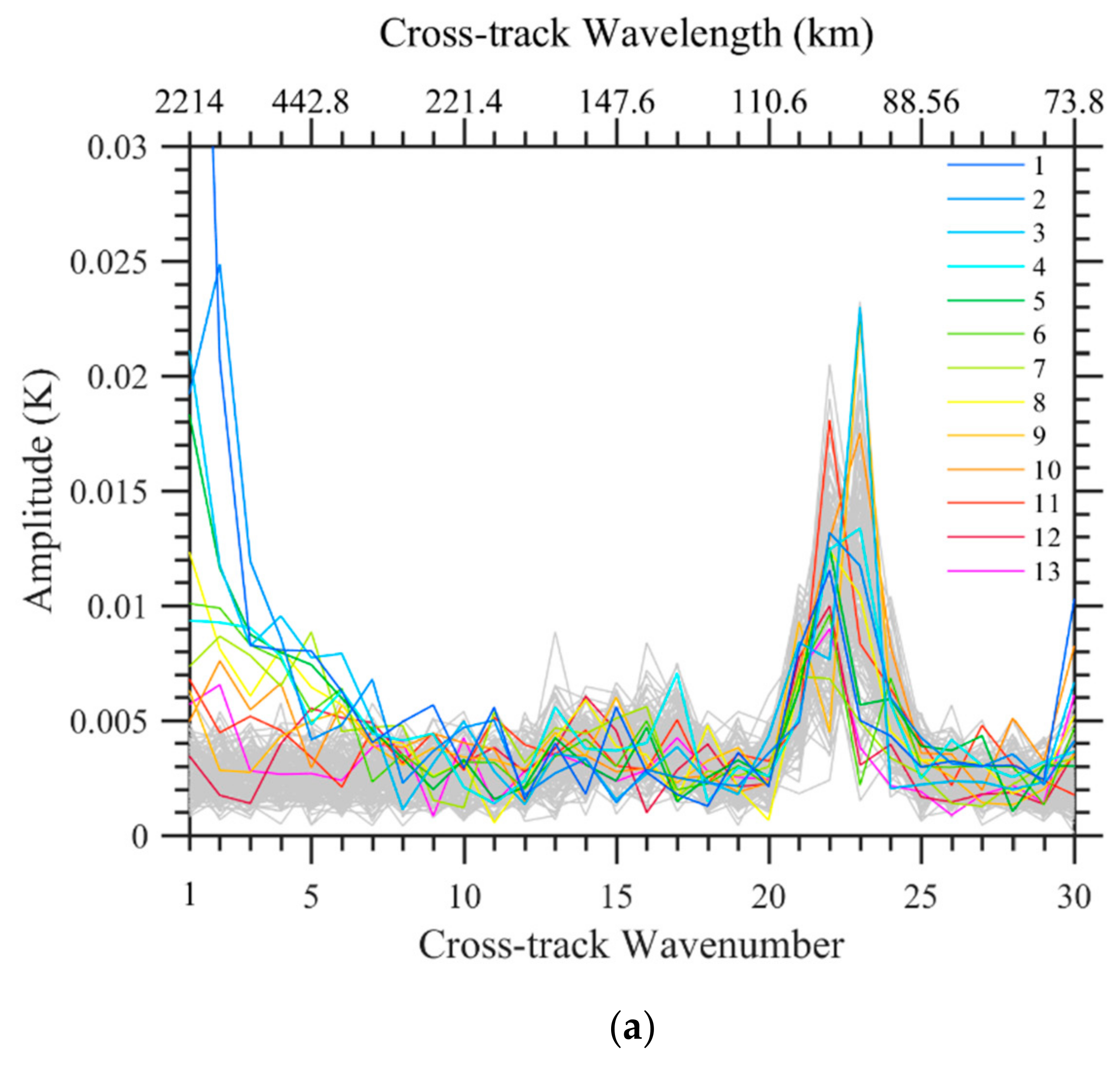
Section 3 was conducted for TB observations in these three areas. Variations of 2D amplitude with respect to wavenumbers in cross- and along-track directions are presented in two ways to provide a qualitative and quantitative look at all waves in
Figure 5 and
Figure 6, respectively. The amplitudes and cross-track wavenumbers shown as the color shading and
y-axis in
Figure 5 are simply switched to the
y-axis and curves in
Figure 6. In
Figure 6, amplitude variations with the along-track wavenumber are represented by a spaghetti map for all 1–150 cross-track wavenumbers in each area. A common spectral feature among TB observations over the three areas is that the amplitudes are the largest near-zero wavenumbers and decrease rapidly with wavenumbers in both across- and along-track directions. However, we also noticed amplitudes at some fixed across-track wavenumbers being higher than their neighboring wavenumbers, which may represent noise signals seen in the left panels of
Figure 4. The exact across-track wavenumbers of these large-amplitude bands are different among these three areas.
The detected noise, defined as the difference between the original and reconstructed TB observations, is shown in
Figure 7. The curvy noise-looking pattern in the TB observations of channel 5 (left panels in
Figure 4) resembles the noise detected in
Figure 7 and disappears in the spatial distribution of TB observations of channel 5 over areas A, B, and C after the noise mitigation (right panels in
Figure 4).
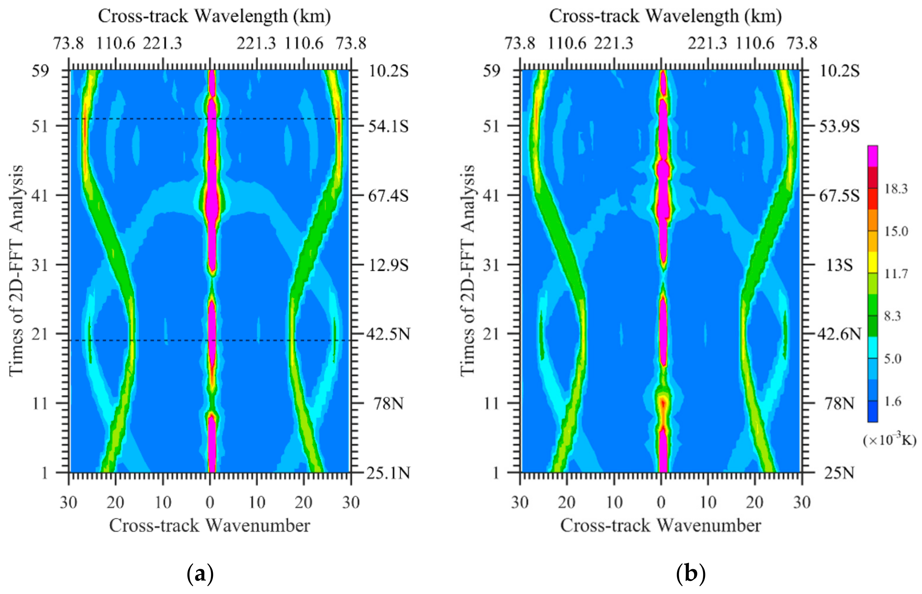
The regional dependence of data noise on across-track wavenumbers is further confirmed in
Figure 8, which shows the along-track variations of 2D amplitude with respect to the cross-track wavenumber for TB observations over the two swaths in
Figure 3. The across-track wavenumbers of larger amplitudes vary along both swaths compared with those of larger and smaller neighboring wavenumbers. We also found that variations of the across-track wavenumbers of data noise with respect to the observing latitude were the same for the two swaths. In other words, the F16 SSMIS LAS channels’ data noise depends on the latitude of the F16 orbit. Bell et al. [
28] reported that solar intrusions into the warm calibration load affect the calibration accuracy for different parts of the orbit, and the thermal cycling of an orbit may also result in a modulation of the measured TB observations by the main reflector emission. The exact root cause for this noise pattern requires further investigation and is beyond the scope of this study.
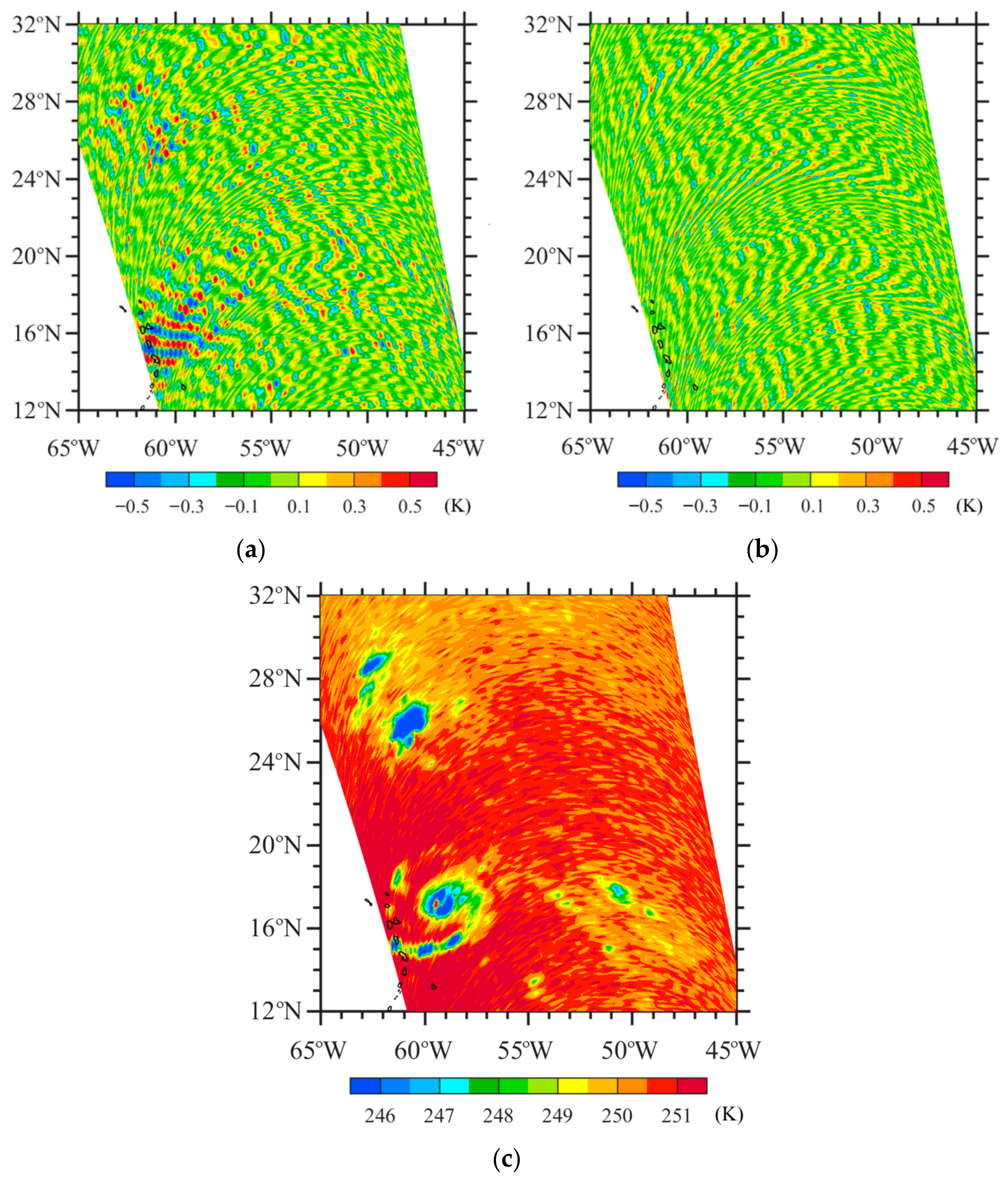
Being sensitive to the atmosphere in the lower altitudes of the middle and lower troposphere than other LAS channels in the upper troposphere and stratosphere, TB observations of LAS channels 1–4 were more strongly affected by cloud and precipitation.
Figure 9 provides an example of channel-3 noise extracted by the same method as channel 5 (
,
Figure 9a). The noise was extracted by adding a step to avoid the impacts of heavy precipitation-induced TB outliers of abnormally small value on the 2D spectrum (
,
Figure 9b), and the reconstructed channel-3 TB observations (i.e.,
) at the ascending node on 5 September 2017 (
Figure 9c). The noise extracted by the same method as channel 5 (
Figure 9a) was not homogeneously distributed in space, with large magnitudes in places of abnormally low TB observations. After adding a step to avoid the impacts of heavy precipitation-induced TB outliers, the noise extracted by the same method as channel 5 (
Figure 9b) was homogeneously distributed in space and resembled those of the upper-level channel 5 (right panels in
Figure 4).
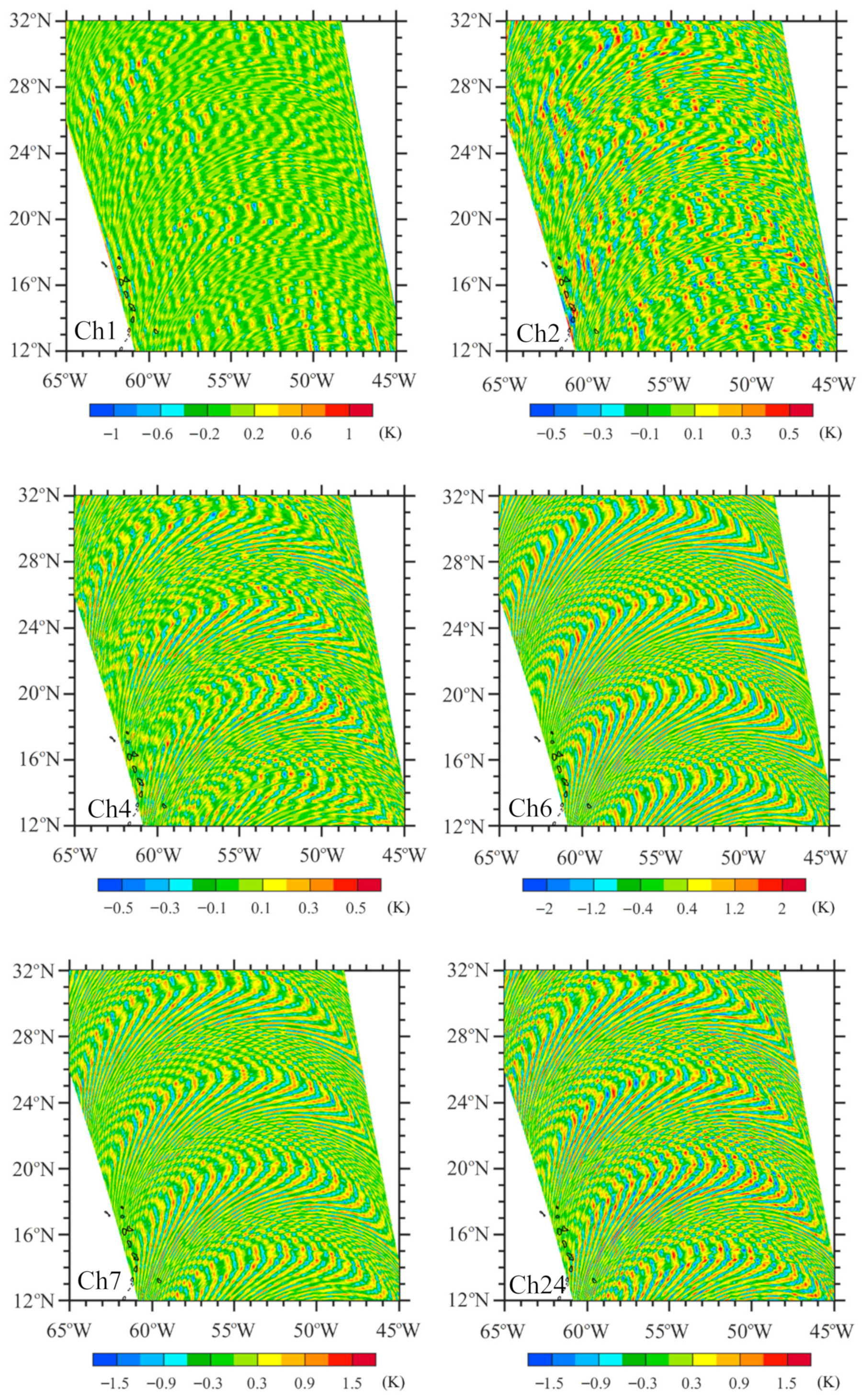
Figure 10 provides the spatial distribution of TB observations after noise reduction for the LAS channels 1–4, 6–7, and 24 over the same swath portion as
Figure 2. The systematic curvy noise pattern seen in
Figure 2 was successfully removed. What remains to be seen in TB observations besides weather signals are random errors, which are 0.4, 0.5, 0.6, and 0.7 for channels 4, 6, 7, and 24 (see
Table 1). The noise detected for channels 1–4, 6–7, and 24 (
Figure 11) have a curvy pattern, as seen in TB observations (
Figure 2).
5. Hurricane Structures Directly Revealed by SSMIS LAS Channels
Hurricanes are characterized by structured bands of cloud and precipitation. Due to the scattering effect by ice particles, TB observations in hurricane rainbands are colder than their surroundings. Therefore, a horizontal TB distribution can reveal hurricane rainband structures. We chose Hurricane Irma (2017) to illustrate TB observations from SSMIS LAS channels’ capability to capture its structures.
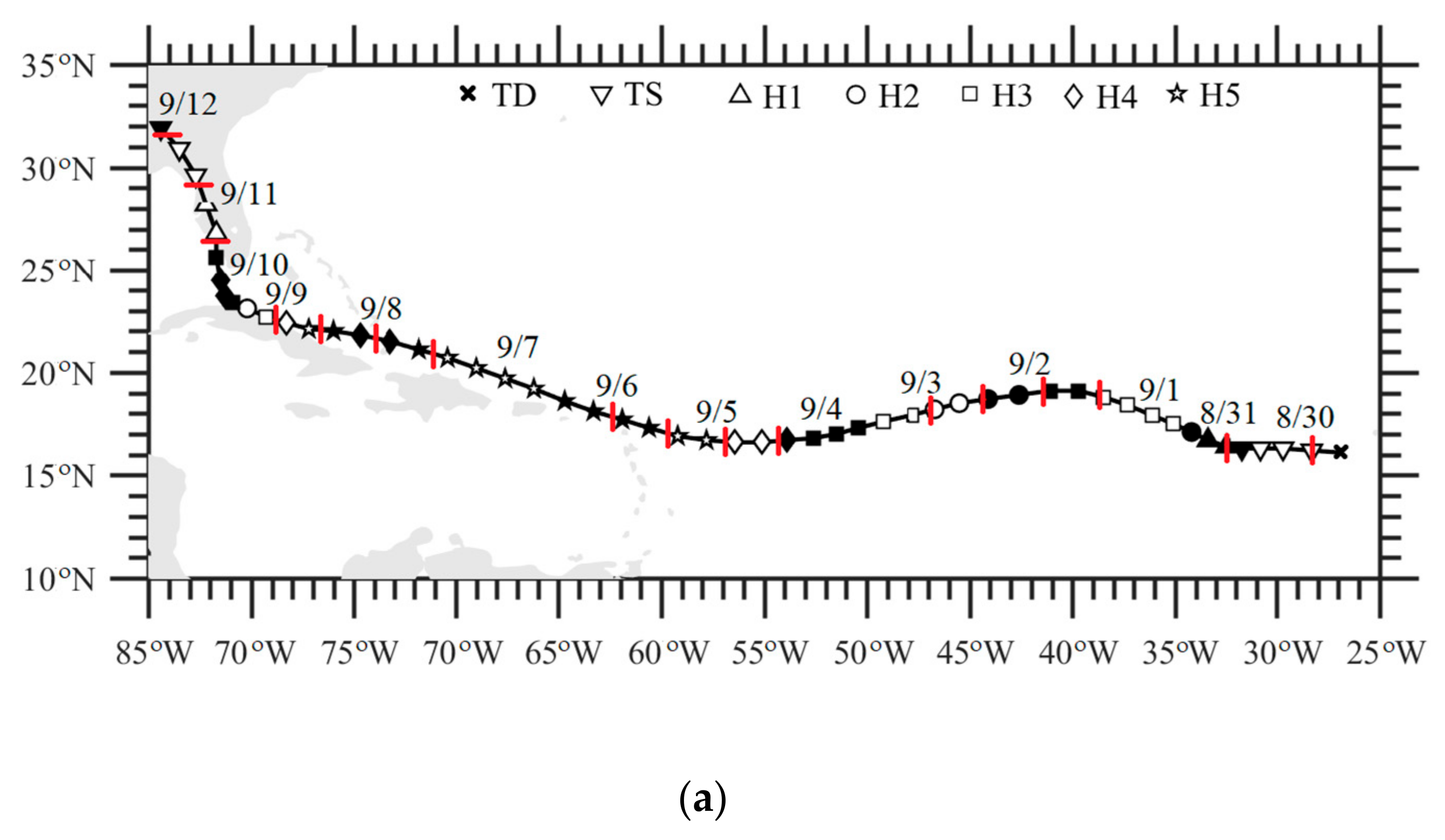
Irma was the most intense hurricane to strike the United States since Katrina in 2005. It originated at low latitudes in the deep tropics on 30 August 2017 and rapidly intensified shortly after its formation. Irma fluctuated between hurricane categories 2 (H2) and 3 (H3) (Saffir–Simpson scale) from 1800 UTC on 31 August to 1800 UTC on 4 September 2017 while experiencing a series of eyewall replacement cycles and reaching category 5 at 1200 UTC 5 September 2017. After its first landfall in Cuba on 9 September 2017 as a category-5 hurricane, Irma made its second and third landfalls in Florida’s Cudjoe Key and Marco Island at H4 and H5 intensities, respectively. It caused widespread and catastrophic property damage and many deaths.
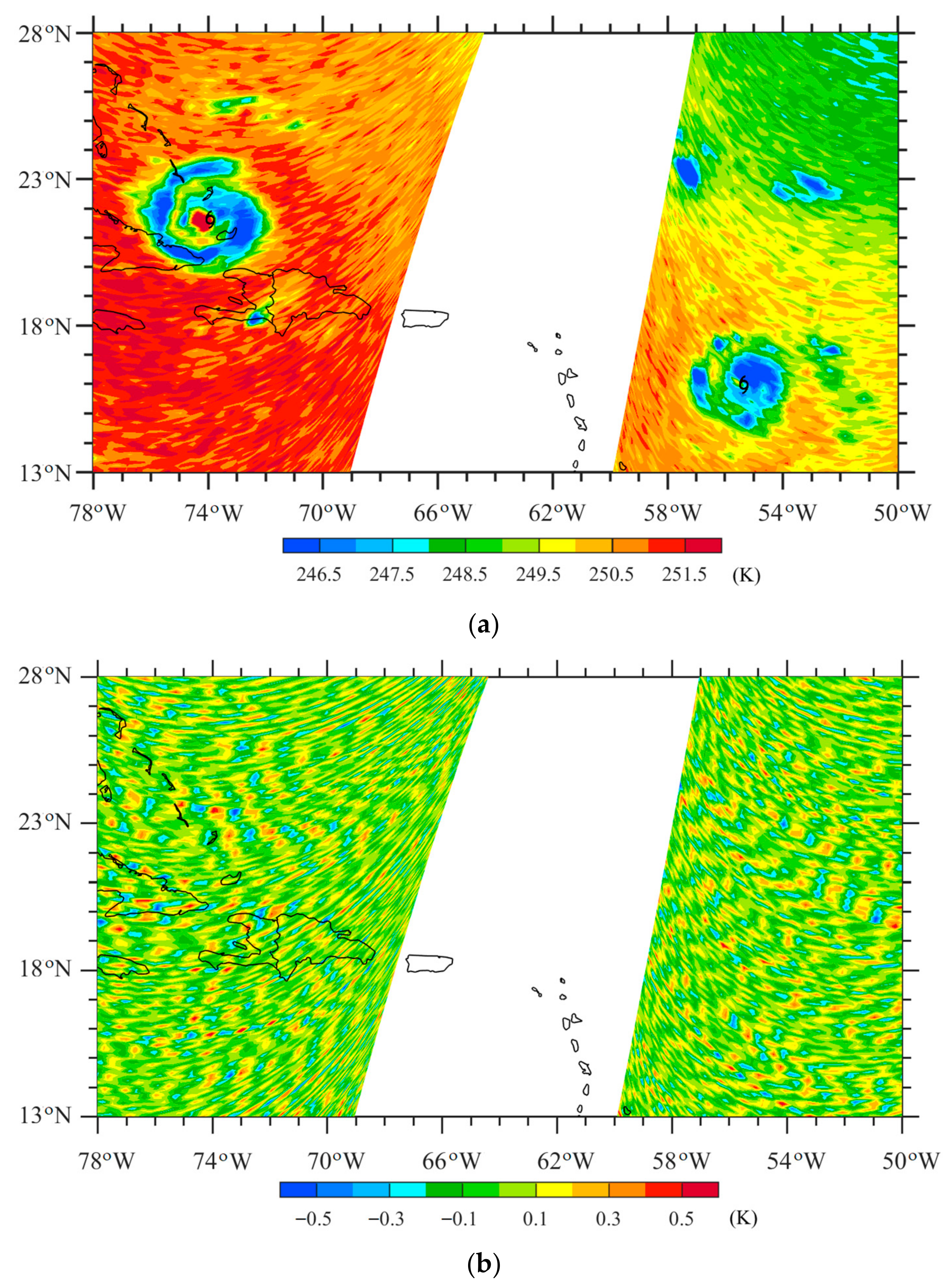
Figure 12a shows the SSMIS TB observations at LAS channel 3 for Hurricanes Irma and Jose; the latter appeared simultaneously with Irma over the Atlantic Ocean in September 2017. Since the detected noise of channel 3 is <0.5K (
Figure 13b), the TB observations after the noise deduction look the same as
Figure 13a, whose color interval is 0.5 K. At 0721 UTC on 8 September, Irma reached H4 intensity and Jose, the hurricane located to the southeast of Irma, was H3. At 0000 UTC on 8 September, the maximum sustained wind speed was 161 and 121 mph for Irma and Jose, respectively. The radius of 34-kt wind speed was 296 and 222 km for Irma and Jose, respectively. In
Figure 13, the west swath captured the structures of Hurricane Irma, and the east swath revealed Hurricane Jose’s structure. A relatively large orbital gap exists between the two swaths. The hurricane eye is identifiable for both Irma and Jose. The observed TB values in the circularly distributed convective rainband regions are more than 6 K lower than those in their eyes, clear streaks between rainbands, and environments. The eye and rainband range of Irma are larger than those of Jose, with a fixed FOV size of 27 × 18 km
2 at a fixed interval between the neighboring FOVs of 12.5 × 37.5 km
2 (see
Table 1). Such hurricane structures cannot be seen directly from TB observations of cross-track temperature sounders due to variations in their FOV size, spacing between two neighboring FOVs, and WF peak altitude along a scanline. Considering AMSU-A as an example, the altitude where the atmosphere contributes the most to an observed TB also increases with scan angle in the troposphere. Spacing between neighboring FOVs also increases with scan angle, and the across-track diameter of an FOV is 48 and 155 km at the nadir and swath edge, respectively [
30]. Even the smallest AMSU-A FOV at the nadir is much coarser than the SSMIS FOV.
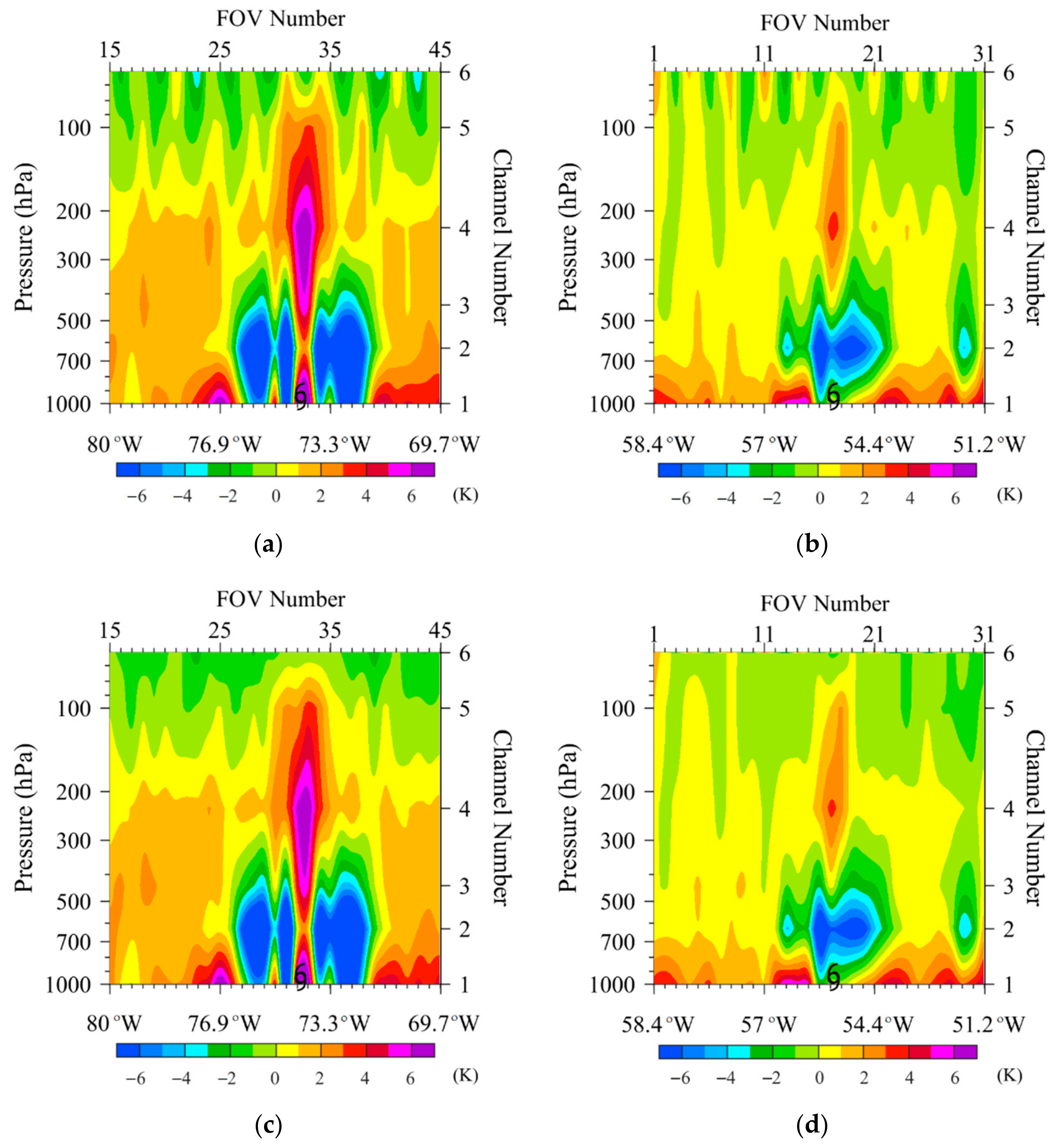
LAS channels were designed for vertically profiling the atmosphere and can be used to examine the vertical structures of hurricanes.
Figure 13 provides vertical cross-sections of TB observations for channels 1–6 along the scanline passing through the center of Hurricane Irma located at (21.6°N, 73.9°W), and along the scanline passing through the center of Hurricane Jose at (15.9°N, 55.3°W). The mean environmental temperature within a latitude–longitude geographic box centered at the same latitude of the hurricane center but away by 1000 km was subtracted to see the warm-core structure more clearly. An unrealistic wave-like structure at a scale of about 112 km is seen in TB observations above 200 hPa without removing detected noise (
Figure 13a,b). The proposed noise detection algorithm successfully removed this noise (
Figure 13c,d). The warm-core maxima of both Irma and Jose are located at about 250 hPa. The Irma warm-core TB is more than 7 K, which is 4 K warmer than Jose. The warm core of Irma went to the ocean surface and extended to 70 hPa, while Jose was confined from 400 to 100 hPa. Significant scattering by precipitation size ice particles was confined below 400 and 500 hPa for Irma and Jose, respectively. Similar cross-sections of TB observations capable of revealing the vertical structures of a hurricane can be determined along any line passing through the hurricane center from the SSMIS LAS observations. However, cross-sections from AMSU-A sounding channel observations can only be determined along a line with a fixed FOV passing through the hurricane center, mainly from south to north directions, slightly tilted westward and eastward for the ascending and descending node, respectively.
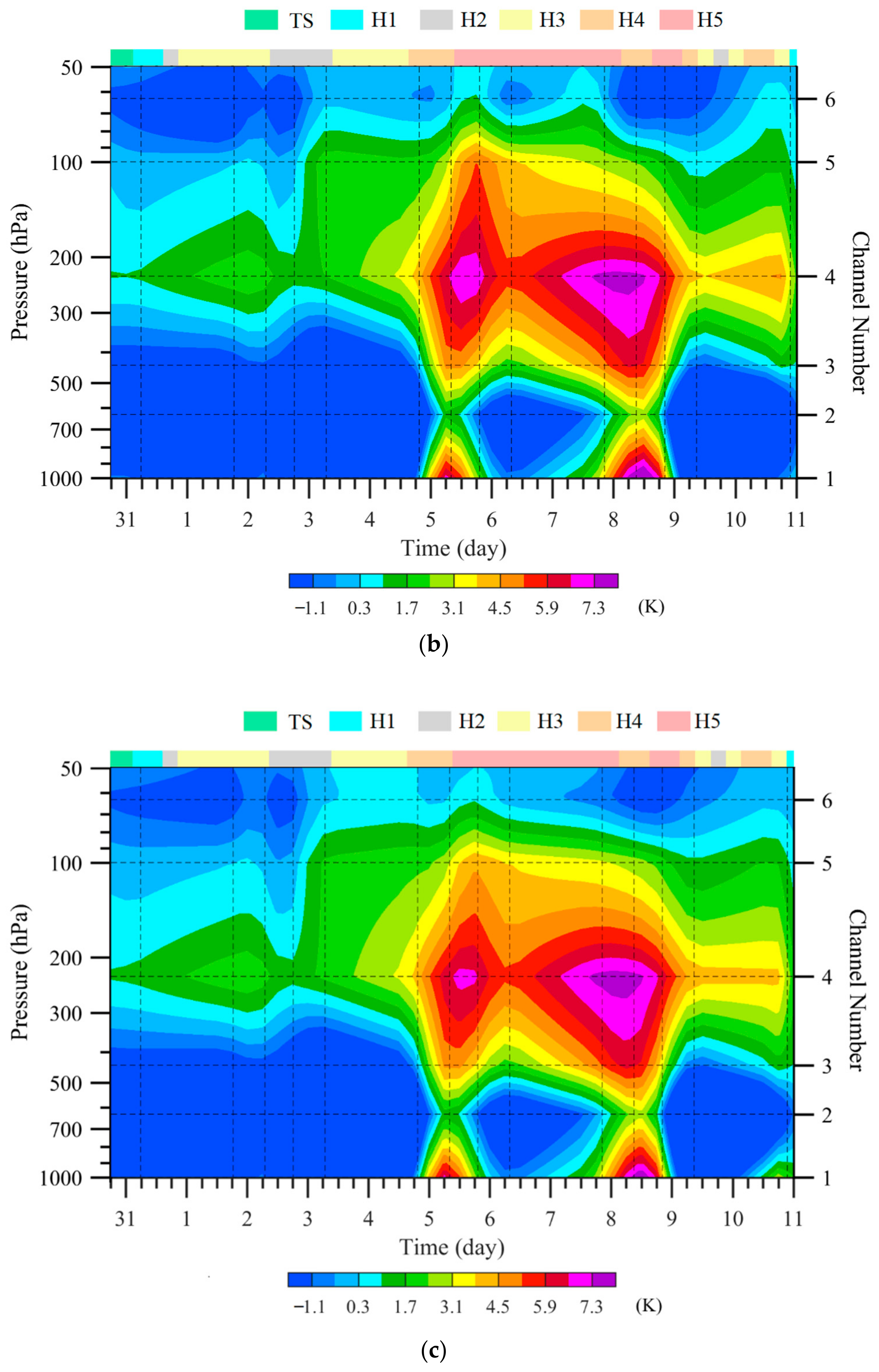
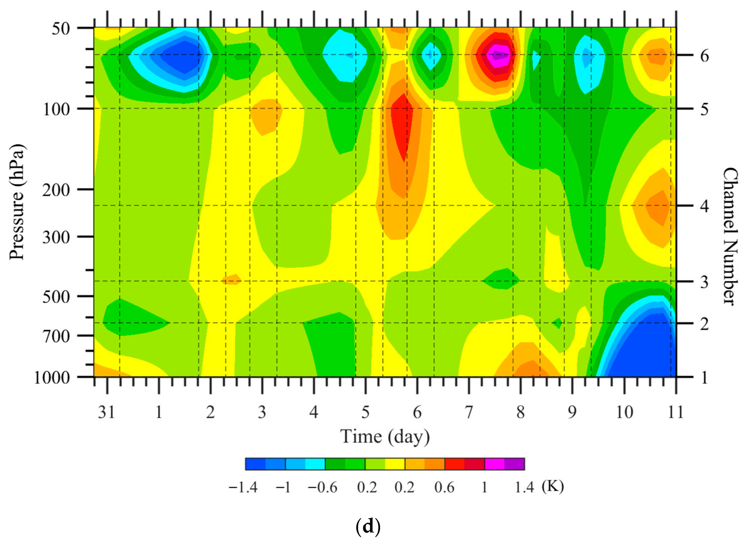
As Hurricane Irma moved along its best track and the intensity changed (see
Figure 14a), the vertical structure also changed, as indicated by TB observations at Irma’s center from 30 August to 11 September 2017 (
Figure 14b,c). The detected noise was less than 1.2 K (
Figure 14d). Here, the TB anomaly is defined as the TB observations subtracted by the mean environmental temperature within a latitude–longitude geographic box centered at the same latitude of the hurricane center but away by 1000 km. Irma’s warm core was maximized at about 250 hPa. As Irma’s intensity increased from 31 August to 5 September 2017 (see Figure 1b in Tian and Zou [
22]), the TB warm-core depth and intensity continually increased from 5 September to 8 September, during which Irma was an H5 hurricane. We noticed that the warm core extended to the surface around 0805 UTC on 5 September and 0910 UTC on 8 September due to Irma’s large clear eye, as shown in
Figure 13 and
Figure 14 for the 0910 UTC on 8 September. Such useful information is difficult to obtain by AMSU-A TB observations or warm-core temperature retrieval due to the AMSU-A’s inability to resolve hurricane eye adequately.
6. Conclusions
The 20-year long-term satellite observations from F16 provide opportunities and challenges for TC study. Using the conical scanning mode, the TB observations from the LAS channels can directly reveal useful information on TC location, intensity, size, and rainband distribution. The challenge is that a systematic data noise appeared after 10 years of F16 operation. We aimed to develop an appropriate method for removing the noise so that the remaining 10 years of F16 SSMIS LAS channel observations can be used together with the first 10 years of high-quality data.
Although it appeared complicated, we found a simple 2D FFT that shows promise for the above-intended purpose. We implemented it to an SSMIS swath in a portion-by-portion manner, where a portion consisted of 300 scanlines. An extra step was added to avoid the impacts of heavy precipitation-induced TB outliers of abnormally small value in TB observations of LAS channels 1–4 during the 2D FFT analysis. For each data portion, the data noise appeared to have larger amplitudes at certain across-track wavenumbers than neighboring wavenumbers (either smaller or larger), which does not vary with the along-track wavenumbers. The across-track wavenumbers of data noise vary and depend on the latitude of the F16 orbit. The magnitude of the noise varies between 0.5 and 2 K depending on the channel number.
The TC features seen in TB observations for SSMIS LAS channels are illustrated for Hurricanes Irma and Jose, along with the impacts of the data noise. We plan to first perform an extensive validation of this technique, especially in the tropics, over a longer period and then extend to all data periods with detected noise. Finally, we will use the 20 years of F16 SSMIS observations for a more substantial study on global TCs at both the synoptic and climate scales.


