
Influence of Terrestrial Water Storage on Flood Potential Index in the Yangtze River Basin, China

 ,
,
Abstract
:1. Introduction
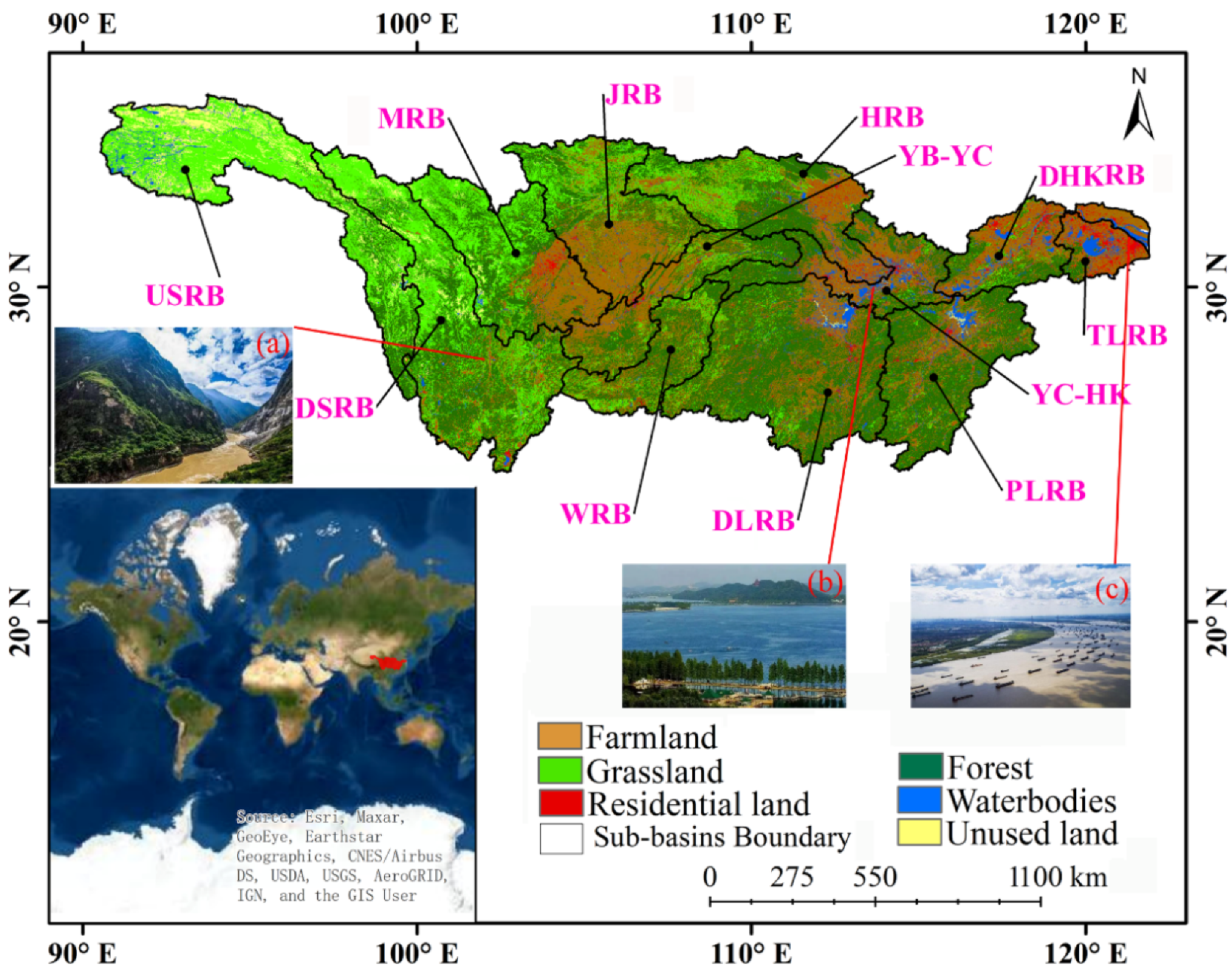
2. Study Area
3. Materials and Methods
3.1. Materials
3.1.1. GRACE Products
3.1.2. Variable Infiltration Capacity (VIC)-Runoff/SM
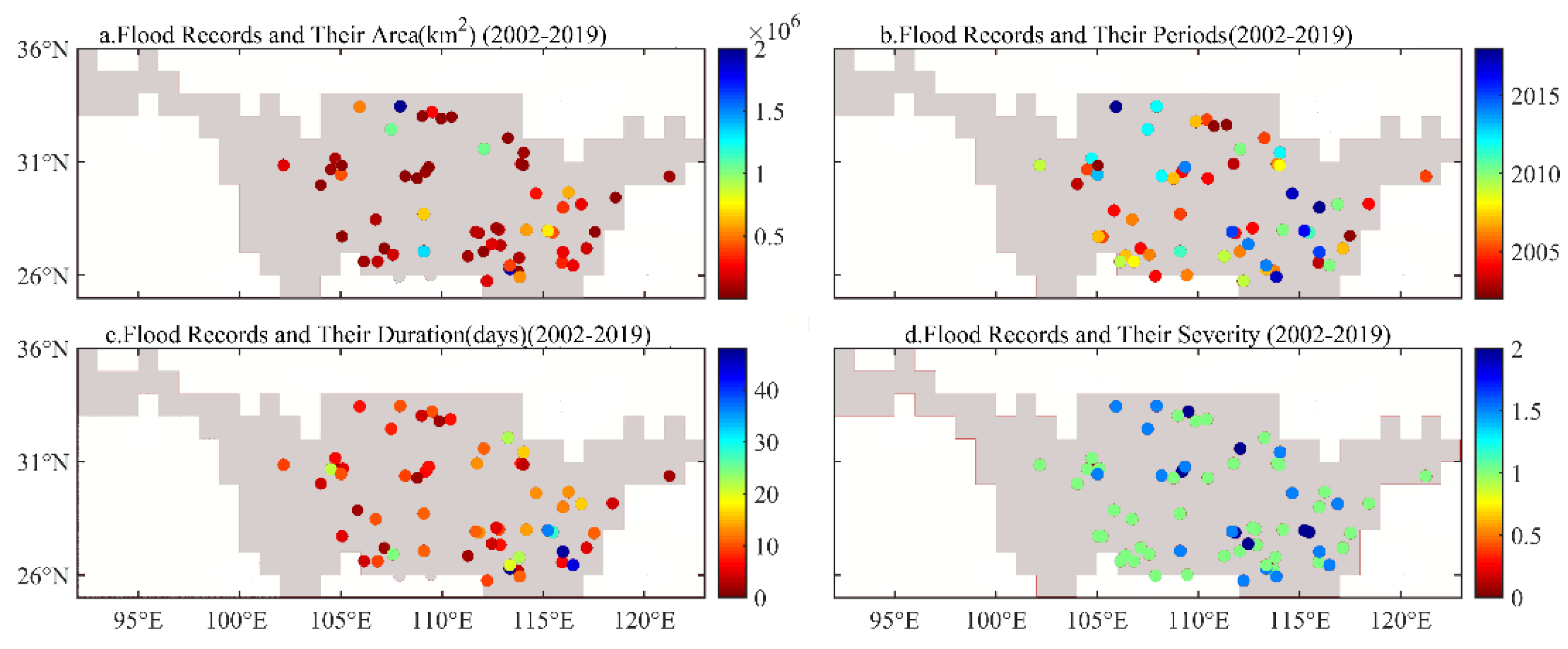
3.1.3. Flood Data
3.1.4. Meteorological Data
3.2. Method
3.2.1. Reconstruction of TWS between GRACE and GRACE-Follow On
3.2.2. Derivation of FPI
3.2.3. Granger Causality Analysis
3.2.4. Standardization Method
3.2.5. Calculation of Relative Contribution
4. Results
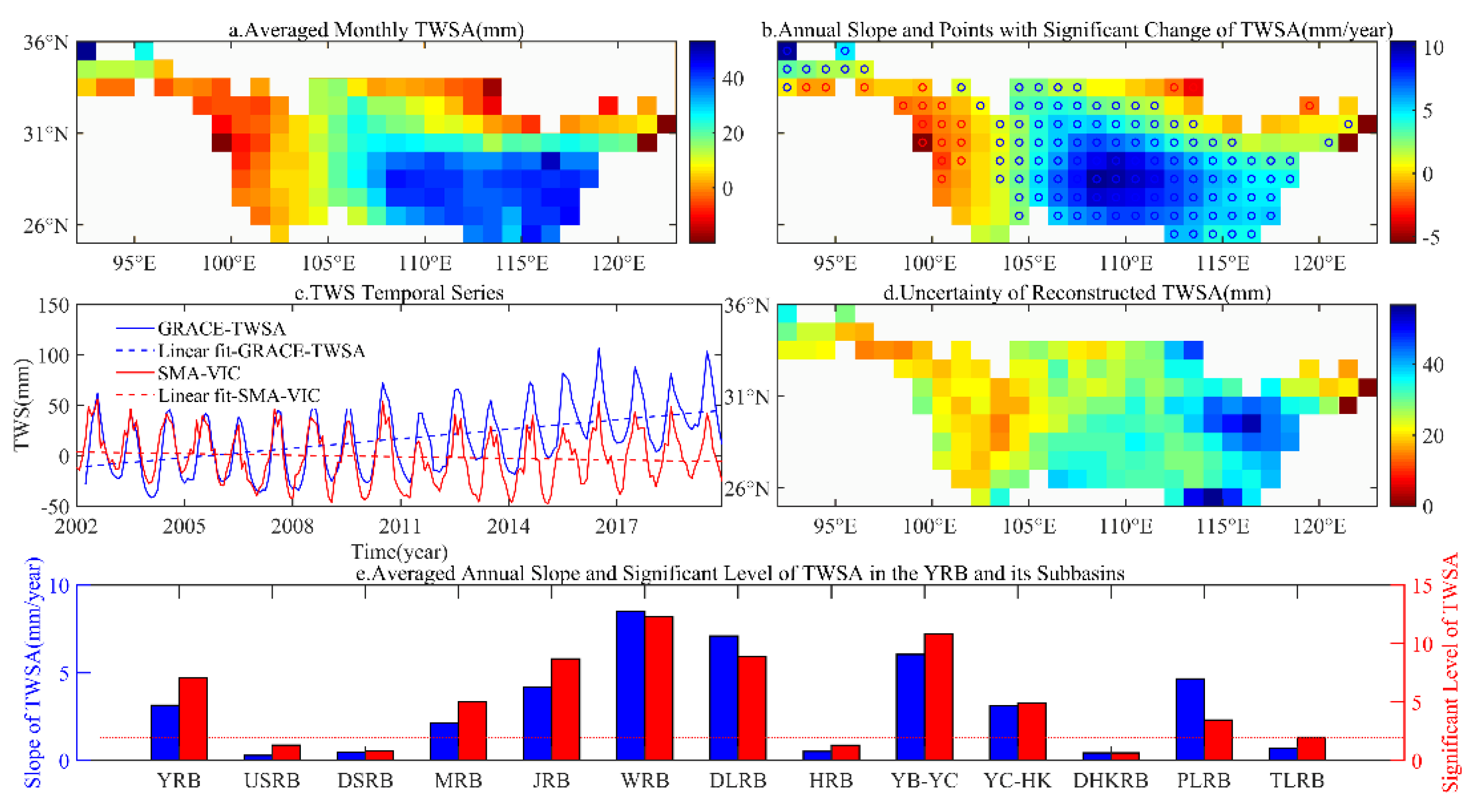
4.1. Characteristic of TWSA in the YRB during April 2002–December 2019
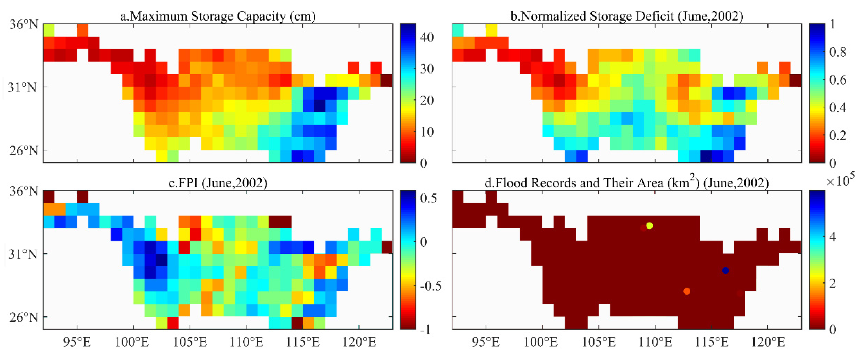
4.2. Derivation of FPI in the YRB
4.3. Impacts of Major Hydrological Factors on the FPI
4.4. Relationship between Extremely Monthly Runoff and Other Major Monthly Hydrological Factors
4.5. Impacts of SM on TWSA in the YRB
5. Discussion
5.1. Why Do TWSA and SMA Increase in the YRB and Its Most Sub-Basins?
5.2. Why Is the Spatial Distribution of Higher Flood Frequency Areas Inconsistent with Smaller MSC?
6. Conclusions
- (1)
- The TWSA in the middle reaches of the YRB showed an obvious increasing trend (p < 0.05), while those in the upper reaches of the Jialingjiang River Basin and Hanjiang River Basin showed an obvious decreasing trend (p < 0.05). However, although the GRACE-TWSA in the YRB showed an increasing trend for the averaged TWSA over all grids in the whole basin, the VIC-SMA showed a decreasing trend (p < 0.05).
- (2)
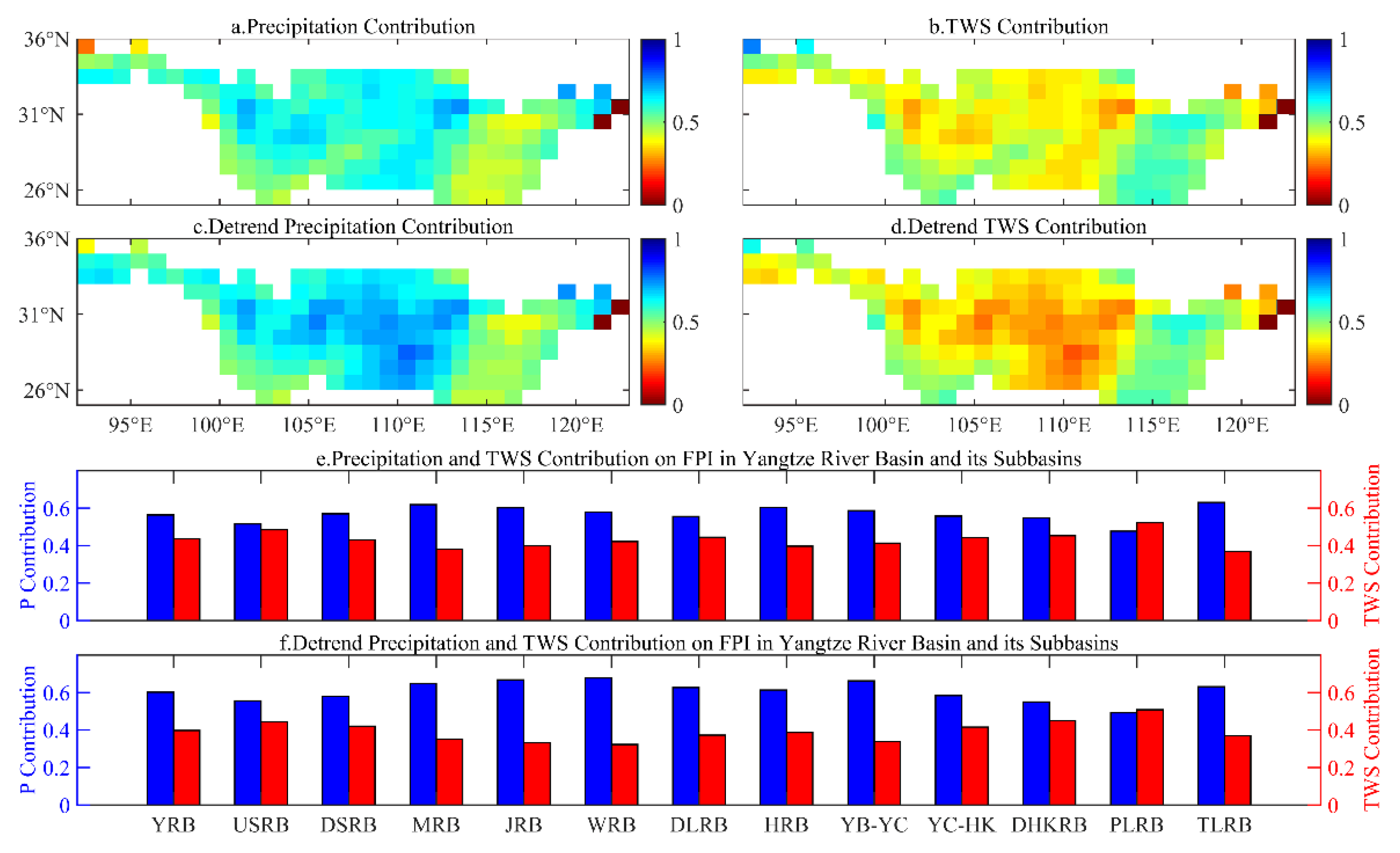
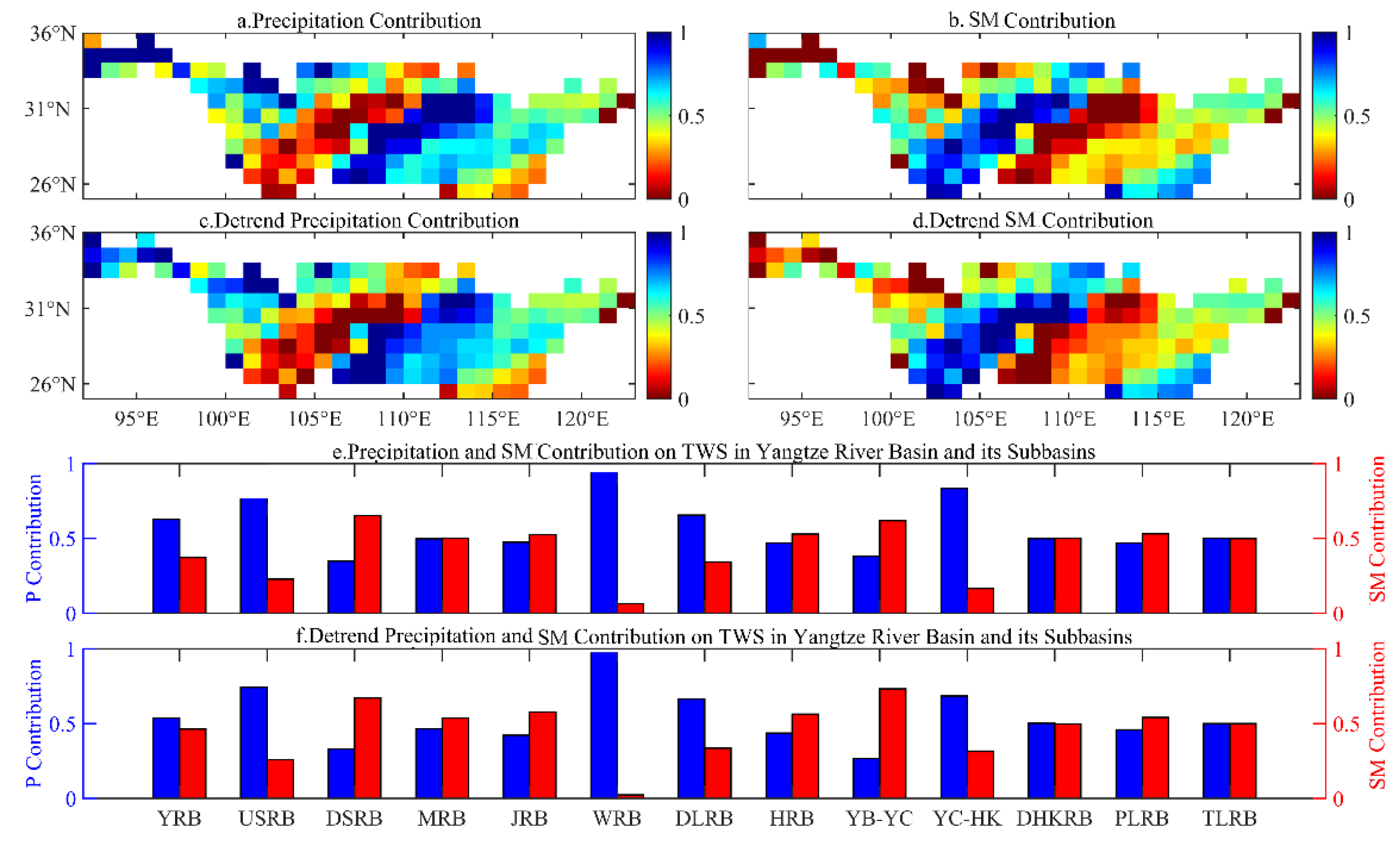
- The relative contribution of precipitation to FPI in the Minjiang River Basin, Hanjiang River Basin, and Dongting Lake River Basin was significantly greater than that in other sub-basins; however, the contribution of TWSA to Poyang Lake Rivers Basin was significantly larger than that in other regions, and the larger relative contribution of detrended precipitation of FPI was found in the Jialingjiang River Basin, Wujiang River Basin, Dongting Lake River Basin, Yibin-Yichang, and Yichang-Hukou, while the contribution of detrended TWSA to FPI in the Poyang Lake Rivers Basin was larger than that in other basins during April 2002–December 2019.
- (3)
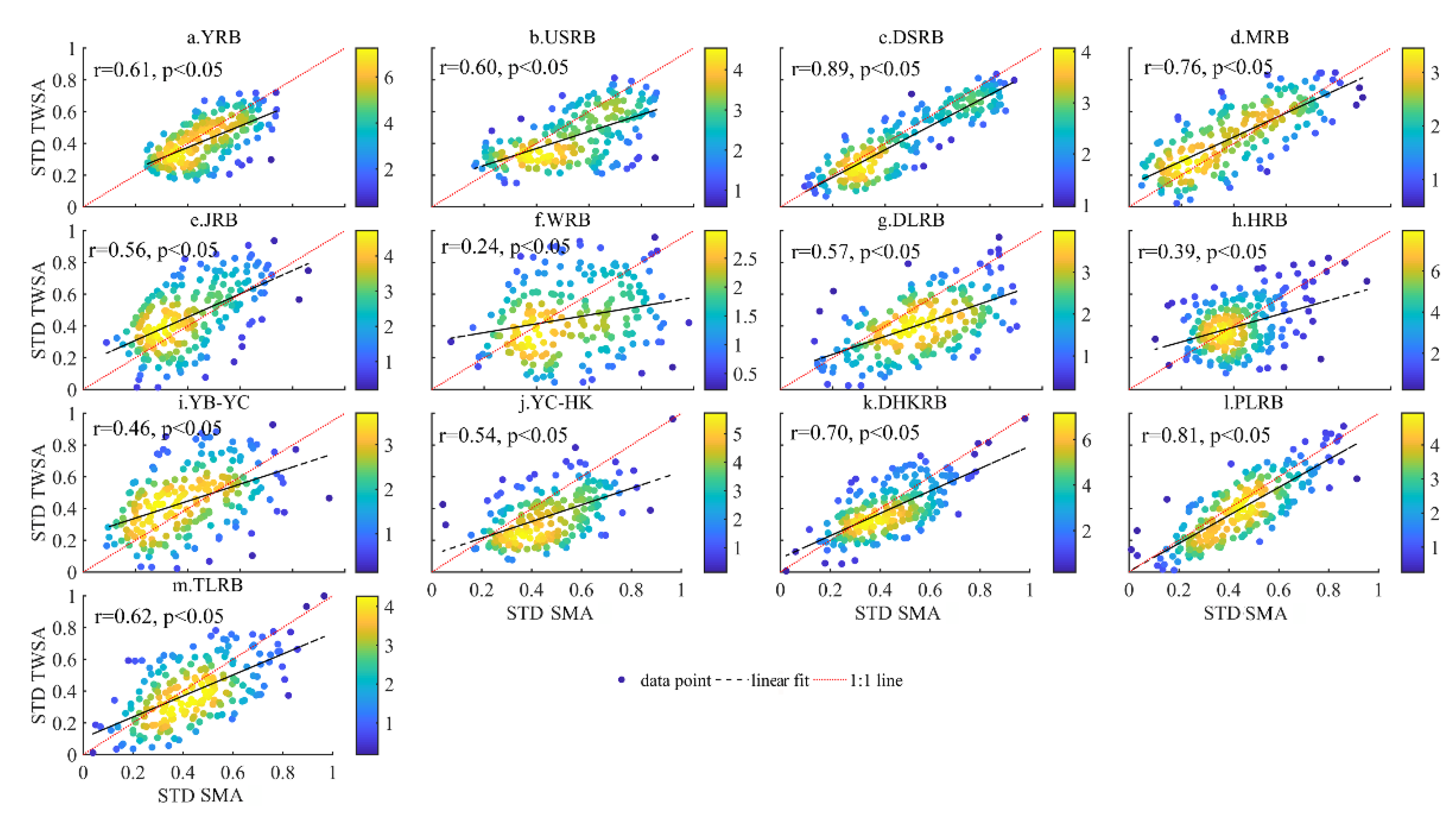
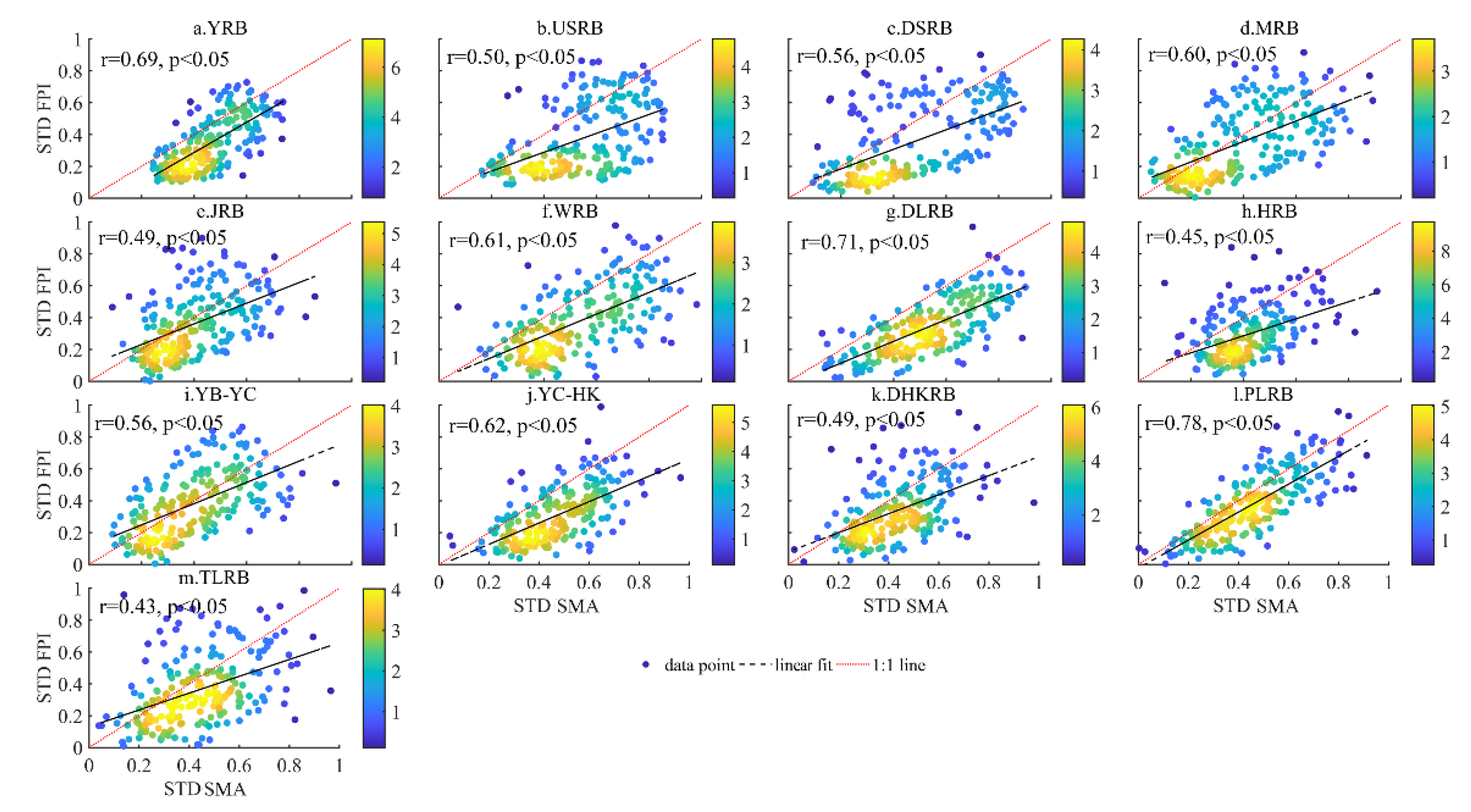
- The contribution of precipitation to the TWSA in the middle-lower reaches of the YRB was significantly greater than that of the SMA, and the relative contribution of the original SMA to TWSA in the upper reaches of the YRB was significantly greater than that of the original precipitation, and the original and detrended SMA and TWSA in the YRB showed a significant positive correlation (p < 0.05), while the significant effect of SM on TWS affected the change in FPI in the YRB and most of its sub-basins.
Author Contributions
Funding
Data Availability Statement
Acknowledgments
Conflicts of Interest
References
- Stefanidis, S.; Stathis, D. Assessment of flood hazard based on natural and anthropogenic factors using analytic hierarchy process (AHP). Nat. Hazards. 2013, 68, 569–585. [Google Scholar] [CrossRef]
- EM-DAT Disaster PProfiles, The OFDA/CRED International Disaster Database. 2020. Available online: http://www.emdat.be/database (accessed on 28 December 2020).
- Wu, C.H.; Huang, G.R.; Yu, H.J. Prediction of extreme floods based on CMIP5 climate models: A case study in the Beijiang River basin, South China. Hydrol. Earth Syst. Sci. 2015, 19, 1385–1399. [Google Scholar] [CrossRef] [Green Version]
- Lai, C.; Chen, X.; Chen, X.; Wang, Z.; Wu, X.; Zhao, S. A fuzzy comprehensive evaluation model for flood risk based on the combination weight of game theory. Nat. Hazards. 2015, 77, 1243–1259. [Google Scholar] [CrossRef]
- Wang, Z.L.; Lai, C.G.; Chen, X.H.; Yang, B.; Zhao, S.W.; Bai, X.Y. Flood hazard risk assessment model based on random forest. J. Hydrol. 2015, 527, 1130–1141. [Google Scholar] [CrossRef]
- Sperotto, A.; Torresan, S.; Gallina, V.; Coppola, E.; Crittoa, A.; Marcomini, A. A multidisciplinary approach to evaluate pluvial floods risk under changing climate: The case study of the municipality of Venice (Italy). Sci. Total Environ. 2016, 562, 1031–1043. [Google Scholar] [CrossRef]
- Gacia, E.; Soto, D.X.; Roig, R.; Catalan, J. Phragmites australis as a dual indicator (air and sediment) of trace metal pollution in wetlands—The key case of Flix reservoir (Ebro River). Sci. Total Environ. 2020, 765, 142789. [Google Scholar] [CrossRef]
- Long, J.L.; Li, H.; Wang, Z.Y.; Wang, B.; Xu, Y.J. Three decadal morphodynamic evolution of a large channel bar in the middle Yangtze River: Influence of natural and anthropogenic interferences. Catena 2021, 199, 105128. [Google Scholar] [CrossRef]
- Dijk, D.V.; Shoaie, S.; Leeuwen, T.V.; Veraverbeke, S. Spectral signature analysis of false positive burned area detection from agricultural harvests using Sentinel-2 data. Int. J. Appl. Earth Obs. 2021, 97, 102296. [Google Scholar]
- Liu, X.M.; Liu, C.; Brutsaert, W. Mutual consistency of groundwater storage changes derived from GRACE and from baseflow recessions in the Central Yangtze River basin. J. Geophys. Res. 2020, 125, e2019JD031467. [Google Scholar] [CrossRef]
- Shah, D.; Mishra, V. Strong influence of changes in terrestrial water storage on flood potential in India. J. Geophys. Res. 2021, 126, e2020JD033566. [Google Scholar] [CrossRef]
- Asoka, A.; Wada, Y.; Fishman, R.; Mishra, V. Strong linkage between precipitation intensity and monsoon season groundwater recharge in India. Geophys. Res. Lett. 2018, 45, 5536–5544. [Google Scholar] [CrossRef] [Green Version]
- Asoka, A.; Mishra, V. Anthropogenic and climate contributions on the changes in terrestrial water storage in India. J. Geophys. Res. 2020, 125, e2020JD032470. [Google Scholar] [CrossRef]
- Tapley, B.D.; Bettadpur, S.; Ries, J.C.; Thompson, P.F.; Watkins, M.M. GRACE measurements of mass variability in the earth system. Science 2004, 305, 503–505. [Google Scholar] [CrossRef] [PubMed] [Green Version]
- Wahr, J.; Swenson, S.; Velicogna, I. Accuracy of GRACE mass estimates. Geophys. Res. Lett. 2006, 33, L06401. [Google Scholar] [CrossRef] [Green Version]
- Chen, J.L.; Wilson, C.R.; Tapley, B.D. The 2009 exceptional Amazon flood and interannual terrestrial water storage change observed by GRACE. Water Resources Res. 2010, 46, W12526. [Google Scholar] [CrossRef] [Green Version]
- Reager, J.T.; Thomas, B.F.; Famiglietti, J.S. River basin flood potential inferred using GRACE gravity observations at several months lead time. Nat. Geosci. 2014, 7, 588–592. [Google Scholar] [CrossRef]
- Scanlon, B.R.; Zhang, Z.; Save, H.; Wiese, D.N.; Landerer, F.W.; Long, D.; Longuevergne, L.; Chen, J. Global evaluation of new GRACE mascons products for hydrologic applications. Water Resour. Res. 2016, 52, 9412–9429. [Google Scholar] [CrossRef]
- Boronina, A.; Ramillien, G.L. Application of AVHRR imagery and GRACE measurements for calculation of actual evapotranspiration over the Quaternary aquifer (Lake Chad basin) and validation. J. Hydrol. 2008, 348, 98–109. [Google Scholar] [CrossRef]
- Rodell, M.; Velicogna, I.; Famiglietti, J.S. Satellite-based estimates of groundwater depletion in India. Nature 2009, 460, 999–1002. [Google Scholar] [CrossRef] [Green Version]
- Strassberg, G.; Scanlon, B.R.; Chambers, D. Evaluation of groundwater storage monitoring with the GRACE satellite: Case study of the High Plains aquifer, central United States. Water Resour. Res. 2009, 45, W05410. [Google Scholar] [CrossRef] [Green Version]
- Syed, T.H.; Famiglietti, J.S.; Chambers, D.P. GRACE-based estimates of terrestrial freshwater discharge from basin to continental scales. J. Hydrometeorol. 2009, 10, 22–40. [Google Scholar] [CrossRef]
- Long, D.; Shen, Y.; Sun, A.; Hong, Y.; Longuevergne, L.; Yang, Y.T.; Li, B.; Chen, L. Drought and flood monitoring for a large karst plateau in Southwest China using extended GRACE data. Remote Sens. Environ. 2014, 155, 145–160. [Google Scholar] [CrossRef]
- Zhang, Q.; Gu, X.; Singh, V.P.; Shi, P.; Luo, M. Timing of floods in southeastern China: Seasonal properties and potential causes. J. Hydrol. 2017, 552, 732–744. [Google Scholar] [CrossRef]
- Reager, J.T.; Famiglietti, J.S. Global terrestrial water storage capacity and flood potential using GRACE. Geophys. Res. Lett. 2009, 36, L23402. [Google Scholar] [CrossRef] [Green Version]
- Famiglietti, J.S. The global groundwater crisis. Nat. Clim. Change 2014, 4, 945–948. [Google Scholar] [CrossRef]
- Yang, P.; Xia, J.; Luo, X.G.; Meng, L.S.; Zhang, S.Q.; Cai, W.; Wang, W.Y. Impacts of climate change-related flood events in the Yangtze River Basin based on multi-source data. Atmos. Res. 2021, 263, 105819. [Google Scholar] [CrossRef]
- Zhong, Y.; Zhong, M.; Mao, Y.; Ji, B. Evaluation of evapotranspiration for exorheic catchments of China during the GRACE Era: From a water balance perspective. Remote Sens. 2020, 12, 511. [Google Scholar] [CrossRef] [Green Version]
- Li, B.Y.; Chen, N.C.; Wang, W.; Wang, C.; Schmitt, R.J.P.; Lin, A.; Daily, G.C. Eco-environmental impacts of dams in the Yangtze River Basin, China. Sci. Total Environ. 2021, 774, 145743. [Google Scholar] [CrossRef]
- Piao, S.; Yin, G.; Tan, J.; Cheng, L.; Huang, M.; Li, Y.; Liu, R.; Mao, J.; Myneni, R.B.; Peng, S.; et al. Detection and attribution of vegetation greening trend in China over the last 30 years. Glob. Change Biol. 2015, 21, 1601–1609. [Google Scholar] [CrossRef]
- Chen, J.; Wu, X.; Finlayson, B.L.; Webber, M.; Wei, T.; Li, M.; Chen, Z. Variability and trend in the hydrology of the Yangtze River, China: Annual precipitation and runoff. J. Hydrol. 2014, 513, 403–412. [Google Scholar] [CrossRef]
- Lü, M.; Wu, S.J.; Chen, J.; Chen, C.; Wen, Z.; Huang, Y. Changes in extreme precipitation in the Yangtze River basin and its association with global mean temperature and ENSO. Int. J. Climatol. 2018, 38, 1989–2005. [Google Scholar] [CrossRef]
- Li, X.; Zhang, K.; Gu, P.; Feng, H.T.; Cheng, B.C. Changes in precipitation extremes in the Yangtze River basin during 1960–2019 and the association with global warming, ENSO, and local effects. Sci. Total Environ. 2021, 760, 144244. [Google Scholar] [CrossRef] [PubMed]
- Fu, B.J.; Wu, B.F.; Lü, Y.H.; Xu, Z.H.; Cao, J.H.; Niu, D. Three Gorges Project: Efforts and challenges for the environment. Prog. Phys. Geog. 2010, 34, 741–754. [Google Scholar] [CrossRef]
- Zheng, L.; Xu, J.; Wang, D.; Xu, G.; Tan, Z.; Xu, L.; Wang, X. Acceleration of vegetation dynamics in hydrologically connected wetlands caused by Dam operation. Hydrol. Processes 2021, 35, e14026. [Google Scholar] [CrossRef]
- Save, H. CSR GRACE RL06 Mascon Solutions (Vol. 1.); Texas Data Repository Data Verse; University of Texas: Austin, TX, USA, 2019. [Google Scholar] [CrossRef]
- Save, H.; Bettadpur, S.; Tapley, B.D. High-resolution CSR GRACE RL05 mascons. J. Geophys. Res. 2016, 121, 7547–7569. [Google Scholar] [CrossRef]
- Beaudoing, H.; Rodell, M. NASA/GSFC/HSL, GLDAS VIC Land Surface Model L4 3 Hourly 1.0 × 1.0 Degree V2.0; Goddard Earth Sciences Data and Information Services Center (GES DISC): Greenbelt, MD, USA, 2020. [Google Scholar]
- Beven, K.J. Rainfall-Runoff Modelling: The Primer, 2nd ed.; John Wiley & Sons: Chichester, UK, 2012. [Google Scholar]
- Humphrey, V.; Gudmundsson, L. GRACE-REC: A reconstruction of climate-driven water storage changes over the last century. Earth Syst. Sci. Data 2019, 11, 1153–1170. [Google Scholar] [CrossRef] [Green Version]
- Granger, C.W.J. Investigating Causal Relations by Econometric Models and Cross-spectral Methods. Econometrica 1969, 37, 424–438. [Google Scholar] [CrossRef]
- Granger, C.W.J. Testing for causality: A personal viewpoint. J. Econ. Dynam. Control. 1980, 2, 329–352. [Google Scholar] [CrossRef]
- Lai, C.; Shao, Q.X.; Chen, X.H.; Wang, Z.L.; Zhou, X.W.; Yang, B.; Zhang, L.L. Flood risk zoning using a rule mining based on ant colony algorithm. J. Hydrol. 2016, 542, 268–280. [Google Scholar] [CrossRef]
- Feng, W.; Zhong, M.; Lemoine, J.M.; Biancale, R.; Hsu, H.T.; Xia, J. Evaluation of groundwater depletion in North China using the Gravity Recovery and Climate Experiment (GRACE) data and ground-based measurements. Water Resour. Res. 2013, 49, 2110–2118. [Google Scholar] [CrossRef]
- Wei, X.; Sun, G.; Liu, S.; Jiang, H.; Zhou, G.; Dai, L. The forest-streamflow relationship in China: A 40-year retrospect. J. Am. Water Resour. As. 2008, 44, 1076–1085. [Google Scholar] [CrossRef] [Green Version]
- Xiao, M.; Zhang, Q.; Singh, V.P. Spatiotemporal variations of extreme precipitation regimes during 1961–2010 and possible teleconnections with climate indices across China. Int. J. Climatol. 2017, 37, 468–479. [Google Scholar] [CrossRef]
- Miao, C.; Duan, Q.; Sun, Q.; Lei, X.; Li, H. Non-uniform changes in different categories of precipitation intensity across China and the associated large-scale circulations. Environ. Res. Lett. 2019, 14, 025004. [Google Scholar] [CrossRef]
- Xiong, J.H.; Yin, J.B.; Guo, S.L.; Xiong, F.; Li, N. Integrated flood potential index for flood monitoring in the GRACE era. J. Hydrol. 2021, 603, 127115. [Google Scholar] [CrossRef]
- Sun, Z.; Zhu, X.; Pan, Y.; Zhang, J. Assessing terrestrial water storage and flood potential using GRACE data in the Yangtze River basin, China. Remote Sens. 2017, 9, 1011. [Google Scholar] [CrossRef] [Green Version]
- Cheng, Q.; Gao, L.; Zuo, X.; Zhong, F. Statistical analyses of spatial and temporal variabilities in total, daytime, and nighttime precipitation indices and of extreme dry/wet association with large-scale circulations of Southwest China, 1961–2016. Atmos. Res. 2019, 219, 166–182. [Google Scholar] [CrossRef]
- Gao, T.; Zhang, Q.; Luo, M. Intensifying effects of El Niño events on winter precipitation extremes in southeastern China. Clim. Dynam. 2020, 54, 631–648. [Google Scholar] [CrossRef]


| No. | Sub-Basins | Short Name |
|---|---|---|
| 1 | Upstream of Jinshajiang-Shigu | USRB |
| 2 | Downstream of Jinshajiang-Shigu | DSRB |
| 3 | Minjiang River Basin | MRB |
| 4 | Jialingjiang River Basin | JRB |
| 5 | Wujiang River Basin | WRB |
| 6 | Yibin-Yichang Reaches | YB-YC |
| 7 | Dongting Lake Rivers Basin | DLRB |
| 8 | Hanjiang River Basin | HRB |
| 9 | Poyang Lake Rivers Basin | PLRB |
| 10 | Yichang-Hukou Reaches | YC-HK |
| 11 | Downstream of Hukou | DHKRB |
| 12 | Taihu Lake Rivers Basin | TLRB |
| Sub-Basin | Lag Month-1 | Lag Month-2 | Lag Month-3 | Lag Month-4 | Lag Month-5 | Lag Month-6 | ||||||
|---|---|---|---|---|---|---|---|---|---|---|---|---|
| F | P | F | P | F | P | F | P | F | P | F | P | |
| YRB | 3.81 | 3.89 | 11.94 | 3.04 | 14.27 | 2.65 | 14.27 | 2.65 | 14.27 | 2.65 | 14.27 | 2.65 |
| USRB | 6.71 | 3.89 | 8.89 | 3.04 | 8.89 | 3.04 | 8.13 | 2.42 | 8.11 | 2.26 | 8.11 | 2.26 |
| DSRB | 47.85 | 3.89 | 17.19 | 3.89 | 10.40 | 3.04 | 12.94 | 3.89 | 8.87 | 3.89 | 8.70 | 3.89 |
| MRB | 2.78 | 3.89 | 59.36 | 3.04 | 44.43 | 2.65 | 44.43 | 2.65 | 43.03 | 2.65 | 41.46 | 2.65 |
| JRB | 1.20 | 3.89 | 13.07 | 3.04 | 13.07 | 3.04 | 5.41 | 3.04 | 4.97 | 2.26 | 7.23 | 2.26 |
| WRB | 21.22 | 3.89 | 0.77 | 3.89 | 0.77 | 3.89 | 4.46 | 2.42 | 1.44 | 3.89 | 5.11 | 2.14 |
| DLRB | 1.36 | 3.89 | 8.59 | 3.04 | 10.63 | 2.65 | 10.63 | 2.65 | 10.63 | 2.65 | 10.63 | 2.65 |
| HRB | 7.10 | 3.89 | 6.19 | 3.89 | 6.19 | 3.89 | 6.19 | 3.89 | 6.19 | 3.89 | 6.19 | 3.89 |
| YB-YC | 7.98 | 3.89 | 20.90 | 3.04 | 18.34 | 2.65 | 13.60 | 2.42 | 9.97 | 2.26 | 7.66 | 2.14 |
| YC-HK | 2.46 | 3.89 | 3.71 | 3.89 | 3.71 | 3.89 | 3.71 | 3.89 | 3.71 | 3.89 | 3.71 | 3.89 |
| DHKRB | 2.62 | 3.89 | 17.24 | 3.04 | 35.06 | 3.89 | 29.03 | 3.89 | 29.03 | 3.89 | 14.62 | 3.89 |
| PLRB | 4.40 | 3.89 | 0.93 | 3.89 | 0.93 | 3.89 | 0.93 | 3.89 | 0.93 | 3.89 | 0.93 | 3.89 |
| TLRB | 6.81 | 3.89 | 5.81 | 3.04 | 9.63 | 3.89 | 9.63 | 3.89 | 9.63 | 3.89 | 6.40 | 3.89 |
| Sub-Basin | Lag Month-1 | Lag Month-2 | Lag Month-3 | Lag Month-4 | Lag Month-5 | Lag Month-6 | ||||||
|---|---|---|---|---|---|---|---|---|---|---|---|---|
| F | P | F | P | F | P | F | P | F | P | F | P | |
| YRB | 42.96 | 3.89 | 36.92 | 3.04 | 10.07 | 2.65 | 5.58 | 2.42 | 4.56 | 3.04 | 4.56 | 3.04 |
| USRB | 28.91 | 3.89 | 32.16 | 3.04 | 17.62 | 2.65 | 16.39 | 2.42 | 14.89 | 2.26 | 8.53 | 2.26 |
| DSRB | 117.21 | 3.89 | 30.21 | 3.04 | 8.43 | 2.65 | 3.62 | 3.89 | 9.56 | 2.26 | 9.36 | 2.14 |
| MRB | 96.42 | 3.89 | 53.89 | 3.04 | 14.34 | 2.65 | 6.34 | 3.04 | 3.30 | 3.04 | 4.81 | 2.14 |
| JRB | 12.10 | 3.89 | 35.20 | 3.04 | 7.22 | 2.65 | 0.65 | 3.89 | 0.17 | 3.89 | 0.17 | 3.89 |
| WRB | 1.11 | 3.89 | 9.66 | 3.04 | 5.53 | 2.65 | 5.80 | 3.89 | 5.55 | 3.04 | 5.55 | 3.04 |
| DLRB | 0.32 | 3.89 | 11.48 | 3.04 | 7.80 | 2.65 | 6.08 | 3.89 | 6.08 | 3.89 | 6.08 | 3.89 |
| HRB | 2.59 | 3.89 | 4.27 | 3.04 | 3.84 | 3.89 | 4.80 | 3.04 | 5.54 | 2.65 | 5.54 | 2.65 |
| YB-YC | 20.93 | 3.89 | 43.98 | 3.04 | 13.41 | 2.65 | 7.55 | 2.65 | 7.55 | 2.65 | 7.55 | 2.65 |
| YC-HK | 0.88 | 3.89 | 9.05 | 3.04 | 7.39 | 2.65 | 4.95 | 3.89 | 1.60 | 3.89 | 1.60 | 3.89 |
| DHKRB | 1.78 | 3.89 | 6.68 | 3.89 | 6.90 | 3.04 | 6.38 | 2.65 | 5.82 | 2.65 | 4.54 | 3.89 |
| PLRB | 5.38 | 3.89 | 11.61 | 3.04 | 11.56 | 3.89 | 2.39 | 3.89 | 2.39 | 3.89 | 2.39 | 3.89 |
| TLRB | 0.25 | 3.89 | 0.25 | 3.89 | 5.70 | 3.89 | 6.75 | 2.65 | 6.75 | 2.65 | 4.92 | 2.65 |
Publisher’s Note: MDPI stays neutral with regard to jurisdictional claims in published maps and institutional affiliations. |
© 2022 by the authors. Licensee MDPI, Basel, Switzerland. This article is an open access article distributed under the terms and conditions of the Creative Commons Attribution (CC BY) license (https://creativecommons.org/licenses/by/4.0/).
Share and Cite
Yang, P.; Wang, W.; Zhai, X.; Xia, J.; Zhong, Y.; Luo, X.; Zhang, S.; Chen, N. Influence of Terrestrial Water Storage on Flood Potential Index in the Yangtze River Basin, China. Remote Sens. 2022, 14, 3082. https://doi.org/10.3390/rs14133082
Yang P, Wang W, Zhai X, Xia J, Zhong Y, Luo X, Zhang S, Chen N. Influence of Terrestrial Water Storage on Flood Potential Index in the Yangtze River Basin, China. Remote Sensing. 2022; 14(13):3082. https://doi.org/10.3390/rs14133082
Chicago/Turabian StyleYang, Peng, Wenyu Wang, Xiaoyan Zhai, Jun Xia, Yulong Zhong, Xiangang Luo, Shengqing Zhang, and Nengcheng Chen. 2022. "Influence of Terrestrial Water Storage on Flood Potential Index in the Yangtze River Basin, China" Remote Sensing 14, no. 13: 3082. https://doi.org/10.3390/rs14133082