Prediction of Potential Geothermal Disaster Areas along the Yunnan–Tibet Railway Project

Abstract

As China’s railways continue to expand into the Qinghai–Tibet Plateau, the number of deep-buried long tunnels is increasing. Tunnel-damaging geothermal disasters have become a common problem in underground engineering. Predicting the potential geothermal disaster areas along the Yunnan–Tibet railway project is conducive to its planning and construction and the realization of the United Nations Sustainable Development Goals (SDGs)—specifically, the industry, innovation and infrastructure goal (SDG 9). In this paper, the Yunnan–Tibet railway project was the study area. Landsat-8 images and other spatial data were used to investigate causes and distributions of geothermal disasters. A collinearity diagnosis of environmental variables was carried out. Twelve environmental variables, such as land surface temperature, were selected to predict potential geothermal disaster areas using four niche models (MaxEnt, Bioclim, Domain and GARP). The prediction results were divided into four levels and had different characteristics. Among them, the area under receiver operating characteristic curve (AUC) and kappa values of the MaxEnt model were the highest, at 0.84 and 0.63, respectively. Its prediction accuracy was the highest and the algorithm results are more suitable for the prediction of geothermal disasters. The prediction results show that the geothermal disaster potential is greatest in the Markam-Deqen, Zuogong-Zayu and Baxoi-Zayu regions. Through jack-knife analysis, it was found that the land surface temperature, active faults, water system distribution and Moho depth are the key environmental predictors of potential geothermal disaster areas. The research results provide a reference for the design and construction of the Yunnan–Tibet railway project and associated sustainable development.

1. Introduction

China is constructing railways in the Qinghai–Tibet Plateau, which will promote economic development and sustainable development goals [1]. Deep-buried long tunnels are required for this railway, which are prone to geothermal disasters. The Sichuan–Tibet Railway is under construction in a Mediterranean Himalayan subtropical zone. Around 15 tunnels are judged to have experienced geothermal disasters. The highest rock temperature measured during the excavation of the Sangzhuling Tunnel on the Lalin Railway was 86 °C. Geothermal disasters deteriorate the construction environment and threaten the health and safety of construction personnel and the efficiency and progress of tunnel projects. They are also detrimental to the safety and durability of tunnel lining structures and the stability and safety of subsequent railway operations [2]. The Yunnan–Tibet railway is located in Southwestern China. It leads northward from Shangri La Station to Deqen County, then extends northwestward to Rawu Station and, finally, connects with the Sichuan–Tibet Railway, which is under construction in Bome County and has a total length of around 490 km [1]. The line crosses the famous “Three Parallel Rivers” area of the Hengduan Mountains. The terrain elevation difference across the whole line is significant, the geological conditions are complex, the ecological environment is fragile, and the project is huge and arduous (Figure 1). Restricted by the topographic elevation difference and geomorphology, the Yunnan–Tibet railway passes through a mountain–canyon area via a tunnel. The construction of a deep-buried long tunnel will greatly reduce the traffic distance and obtain a large decrease in elevation within a short distance, but will inevitably face a series of geological disasters, especially geothermal disasters [3]. Achieving the United Nations Sustainable Development Goals (SDGs) is desirable by governments and society. The industry, innovation and infrastructure goals (SDG 9) emphasize the building of disaster-resistant infrastructure. The sustainable cities and communities goal (SDG 11) calls for the building of inclusive, safe, disaster-resilient and sustainable cities and human settlements. Therefore, the construction of infrastructure such as railways plays a vital role in achieving the SDGs [4,5].

There have been many studies of geothermal disasters in plateau-based linear engineering projects such as the Yunnan–Tibet railway. For example, Yan Jian studied the characteristics of high ground temperatures in the Sangzhuling tunnel of the Sichuan–Tibet Railway in 2019 and analyzed its impact on tunnel engineering [6]. Luo Feng analyzed the ground temperature characteristics of an underground project in the north wall of the Lhari fault on the Qinghai–Tibet Plateau in 2021 and summarized its relationship with the Lhari fault [7]. In addition, research on the influences on geothermal disasters shows that the ground temperature and ground temperature gradient characteristics are closely related to earth thermal processes, tectonism, climate change and formation lithology [8,9,10,11]. However, most of the above studies have focused on the influences of ground temperature distributions and geothermal disasters on engineering projects, while few have predicted potential geothermal disaster areas. The terrain along the Yunnan–Tibet railway project is difficult and dangerous and much of the area is covered by ice and snow, making it very difficult to conduct conventional large-area ground geothermal surveys. Instead, satellite-acquired thermal infrared remote sensing images can provide high monitoring accuracy and are relatively unrestricted by ground conditions. Accordingly, we used them to determine ground temperature anomalies in the study area. Using the GIS platform and spatial information technology, predictive models, such as the evidence weight, deterministic coefficient, maximum entropy and random forest methods, have been used in many fields, such as for the prediction of metallogenic provinces, landslide disasters, suitable species habitats and geothermal resources [12,13,14,15]. For example, Zhang Shuai used a maximum entropy and random forest model to predict the presence of gold deposits in the West Qinling region of China in 2018 [16]. In 2020, Abuzied used Bayesian statistical models in the coastal area of the Gulf of Suez, Egypt, to identify potential geothermal areas [17]. In 2021, Abdel-Fattah pointed out the possible locations of geothermal reservoirs by using information value and evidence weight analyses [18]. In earlier research, we used eight environmental variables to construct a traditional entropy weight information model and an evidence weight information model of geothermal anomalies along the Sichuan–Tibet railway in China [19]. On the basis of previous research, this study analyzed the causes of disasters along the Yunnan–Tibet railway, increased the number of environmental variables to 15, introduced an emerging niche model for prediction and, finally, defined key areas for analysis. The niche model was initially applied to species prediction and analysis. In recent years, it has been widely used to predict the distribution ranges of disasters such as landslides, debris flows and floods [16]. Using data on the known distribution of disasters and disaster-causing environmental variables, the model uses an algorithm to project operation results into different times and spaces to predict potential disaster-prone areas [20]. When the niche model is applied to the prediction of potential areas of geothermal disaster, the known geothermal spots in the study area are considered equivalent to the known distribution data of disasters, and the corresponding environmental variables are the structural prediction variables. At present, there are many commonly used niche models. Each model can independently predict potential disaster-prone areas, but each has a certain preference [21]. Using the idea of an ensemble prediction system and integrating the prediction results of various models, the false-negative or false-positive risk of using a single model can be reduced as much as possible. At the same time, the defects in one model may be compensated for by another model to improve the robustness of prediction [22,23].

Based on niche models that use four different algorithms (MaxEnt, Bioclim, Domain and GARP), taking 15 disaster-causing factors as environmental variables, and in combination with the ArcGIS platform, this study predicts potential areas of geothermal disaster along the proposed Yunnan–Tibet railway project. It compares the prediction results of different models, analyzes the relationships between geothermal disasters and environmental variables and reveals the dominant factors determining the potential distributions of geothermal disasters. It provides a scientific basis and technical support for the engineering planning, route optimization and sustainable development of the Yunnan–Tibet railway. It also provides a reference for the survey, design and engineering construction of complex and dangerous mountainous railways in areas such as Sichuan–Tibet, China–Nepal and Xinjiang–Tibet.

2. Materials and Methods

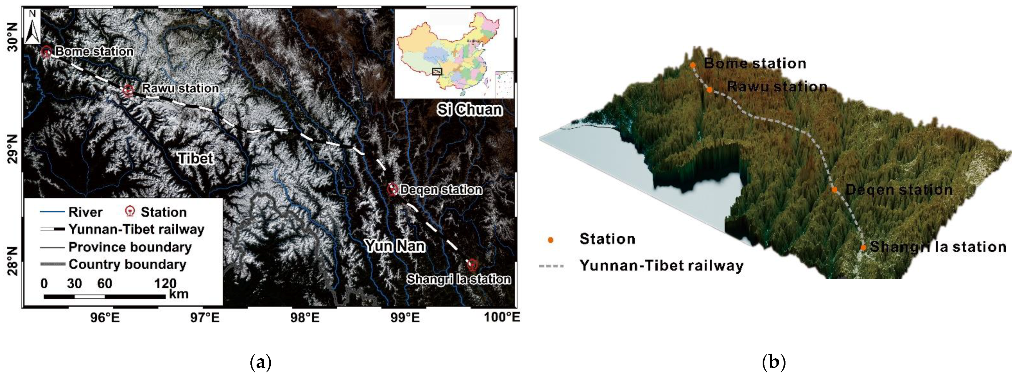
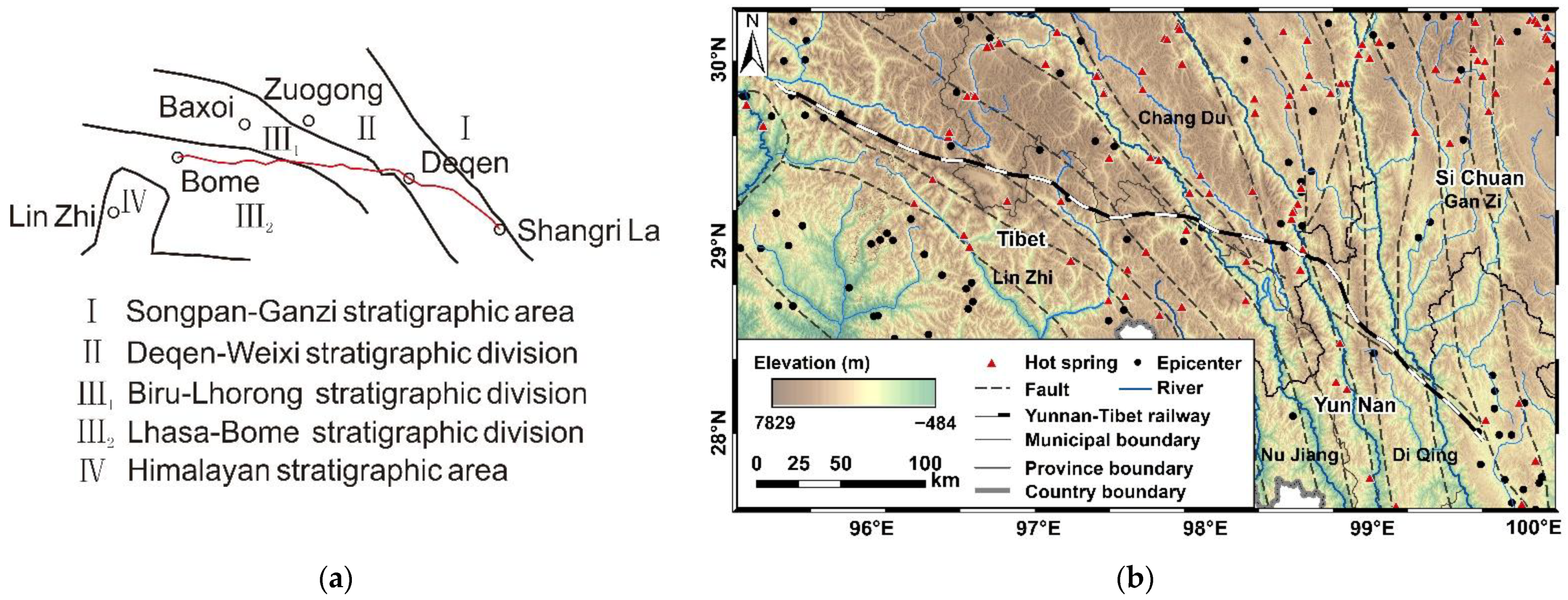
2.1. Study Area

The area was located in Southwest China along the Yunnan–Tibet railway between 27°25′–30°05′N and 95°15′–100°15′E. It includes the Southeastern Tibet Tibetan Autonomous Region and Northern Yunnan Province and covers an area of approximately 143,009 km² (Figure 1). This area has a plateau humid monsoon climate with an annual average temperature of 6.3–12.5 °C, a large daily temperature difference and a minimum temperature of –27.4 °C. The whole year is dry and wet, with an average annual rainfall of 449.19–726.4 mm, which is concentrated from May to September. The railway line passes through four geomorphic units: the Zhongdian fault depression basin area, the Hengduan Mountain high mountain canyon area, the Southeast Tibet high mountain deep canyon area and the Parlung Zangbo River Valley area. The trend of the mountain range is consistent with that of the regional structural belt. The landform has alternating gullies and mountains, and the terrain is generally high in the northwest and low in the southeast. The elevation of the river valley is 2700–3300 m, that of the mountains is 3000–6700 m, and the relative height difference is 1000–3000 m. The canyon areas are mostly V-shaped with cutting depths of 1000–2000 m and bank slope gradients of 30–70° on both sides. Meili Snow Mountain is the highest peak near the line, with an altitude of around 6740 m [1]. The basic topographic conditions are shown in Figure 1.

The eastern part of the study area is the Deqen-Weixi stratigraphic division of the Qiangtang-Qamdo stratigraphic area, and the central and western parts are the Biru-Lhorong and Lhasa-Bome stratigraphic divisions of the Gangdise-Nianqing Tanggula stratigraphic area (Figure 2). The exposed strata are Quaternary to Precambrian, and their distribution is mainly controlled by their structure. The Quaternary strata are mainly sandy soil, gravel soil and cohesive soil; the underlying sedimentary rocks, metamorphic rocks and intrusive rocks are distributed alternately, and the lithology is mixed and changeable [24]. Due to the strong collision and compression of plates and the uplift of the Qinghai–Tibet Plateau, the fault zones in the region are extremely developed and include the Jinsha River fault zone, Lancang River fault zone, Bangong Lake Nujiang suture zone, Jiali fault zone and Yarlung Zangbo River suture zone. The Yunnan–Tibet railway passes through six faults, which, from west to east, are the Deqen Zhongdian fault, Jinshajiang fault, Lancang River fault, Basu fault, Nujiang fault and Lhari fault (Figure 2). The area is characterized by its large scale and fault bandwidth, strong tectonic environment, complex structure and strong activities since the Holocene. It has a seismogenic structure of medium–strong and mega-earthquakes, with the risk of strong earthquakes, and the engineering geological conditions are extremely complex [25]. The engineering problems caused by active faults mainly include catastrophic structural creep and dislocation-induced earthquakes, resulting in secondary disasters such as slope instability and destructive debris flows, and the harm of high-temperature hot springs distributed along the fault zone.

The railway runs through the Yunnan–Tibet geothermal zone in the great bend geothermal activity area of Yarlung Zangbo. It belongs to the Himalayan geothermal zone, which has the strongest geothermal activity in Mainland China. Geothermal activity is mainly distributed in beads along active fault zones or is exposed in fault basins and fault valleys. The geothermal outcrops along the line are mainly hot springs with low salinity. The maximum water temperature exceeds 80 °C and is relatively stable and unaffected by climate. It is an area with an extremely high land surface temperature [26] (Figure 2). The line crosses many seismic zones, such as the Xianshuihe East Yunnan seismic zone, Southwest Yunnan seismic zone, Central Tibet seismic zone and Himalayan seismic zone. It is the largest seismic area in China and is extremely active, with frequent high-intensity earthquakes [27]. The epicenter in Figure 2 is the center of earthquakes with magnitudes ≥ 4 that occurred in the study area from 2300 BC to AD 2000.

The distribution of the river system along the line is controlled by the structure, and its flow direction is consistent with the structural trend (Figure 2). The railway crosses the Jinsha, Lancang, Nujiang and Parlung Zangbo Rivers, among others, from east to west. Water is abundant and seasonal. The runoff is greatest in summer, the rivers are highly sloped, and the water flow is turbulent. Rivers are mainly recharged by precipitation, groundwater and ice meltwater [1]. The fault, hot spring, epicenter and water system data were obtained from the China Geological Survey (https://geocloud.cgs.gov.cn/, accessed on 1 March 2022).

Shallow geothermal energy resources are abundant in the area. Their generation is closely related to the strong solar radiation, complex geological and geomorphic conditions and extreme natural climate of the area. At the same time, they are restricted by geological conditions such as stratigraphic structure, structure, groundwater distribution and rock thermophysical properties [28,29,30]. Under certain circumstances, under the influences of deep heat sources and fractures, places with abundant high temperatures at shallow depths are potential locations of geothermal disasters that could affect the tunnel [11].

2.2. Materials

2.2.1. Geothermal Sample Points

The Yunnan–Tibet tropical zone is located at the collision junction of the Indian Ocean and Eurasian plates. It has the characteristics of long extension distance, grand scale and strong geothermal activity. Hot springs in this area account for more than half of the total number in China. The distribution of abnormal areas of geothermal activity along the railway is related to the activity of active faults. The hot springs exposed on the surface can be regarded as the ground characterization of geothermal disasters. Within an area of 10 km², they may belong to the same geothermal system, and high-temperature hot springs are likely to be concentrated. Therefore, the hot spring points exposed at the surface in the study area were taken as known geothermal sampling points for the predictive model [12]. The data on geothermal sampling points were obtained from a 1:4 million scale map of geothermal resources in China [31], from which 108 geothermal sampling points were selected (Figure 2). Among them, 75% of the points were randomly selected as a training set, and the remaining 25% of sampling points as well as random background points (10 times the number of total sampling points) were selected as the test set. To compare the differences in the predictions of the four models, 10 groups of training datasets and corresponding test datasets were randomly generated. The training set was used for model prediction and the test set was used for model verification.

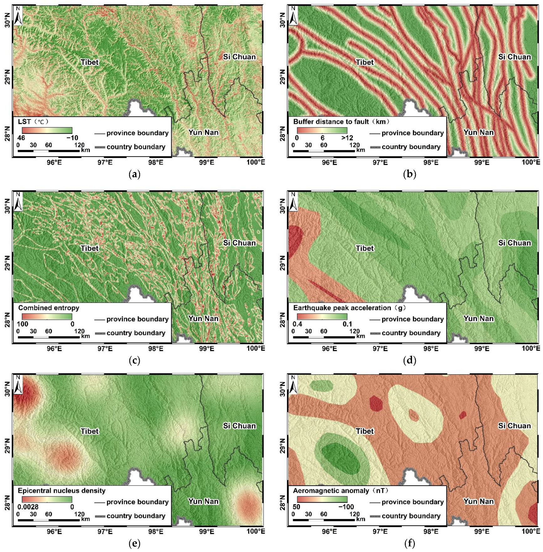
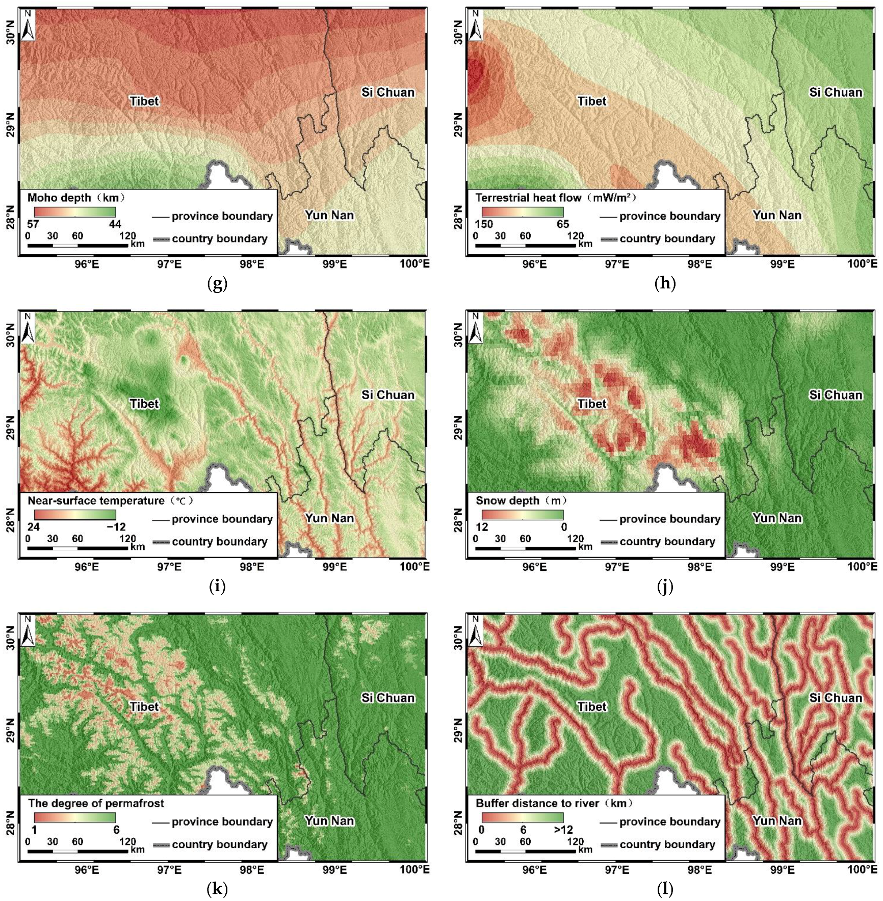
2.2.2. Selection and Processing of Environmental Variables

Considering the geological structure, geophysics, natural climate, landform and hydrogeological conditions of the study area [12], 15 factors were selected as environmental variables: land surface temperature, buffer distance to fault, fault density, combined entropy of geological formation, earthquake peak acceleration, epicentral nucleus density, aeromagnetic anomaly, Bouguer gravity anomaly, Moho depth, terrestrial heat flow, near-surface temperature, snow depth, degree of permafrost, amount of precipitation and buffer distance to a river (

Table 1. Environmental variables.

Code	Environment Variable	Unit
Bio1	Land surface temperature	℃
Bio2	Buffer distance to fault	km
Bio3	Fault density	km/km2
Bio4	Combined entropy of geological formation	-
Bio5	Earthquake peak acceleration	g
Bio6	Epicentral nucleus density	-
Bio7	Aeromagnetic anomaly	nT
Bio8	Bouguer gravity anomaly	mgal
Bio9	Moho depth	km
Bio10	Terrestrial heat flow	mW/m2
Bio11	Near-surface temperature	℃
Bio12	Snow depth	m
Bio13	The degree of permafrost	-
Bio14	Amount of precipitation	mm
Bio15	Buffer distance to river	km

).

The land surface temperature (LST) can provide high-quality and high-efficiency heat information on the land surface and provide a basis for the prediction of geothermal disasters. The terrain of the study area is complex and covers a large area. One of the most effective methods is to obtain surface temperatures through thermal infrared remote sensing inversion [12]. The Landsat-8 satellite has a thermal infrared sensor with a 100 m spatial resolution. From its L1T level data, the land surface temperature anomalies in the study area were extracted with high quality and efficiency. Thermal infrared data were obtained from the U.S. Geological Survey (https://earthexplorer.usgs.gov/, accessed on 1 March 2022) [12]. Finally, the single-window algorithm was used to retrieve the surface temperatures according to the formula

T_s = {a(1 − C_i − D_i) + [b(1 − C_i − D_i) + C_i + D_i]T_b − D_i T_a}/C_i

(1)

$$C_i{=\epsilon }_i{\tau }_i$$

(2)

$$D_i=\left({1 - \tau }_i\right)\left[{1+\tau }_i\left({1 - \epsilon }_i\right)\right]$$

(3)

where a and b are linear regression coefficients related to the temperature range in the study area, C and D are intermediate variables, T_a is the average atmospheric temperature (K), T_b is the brightness temperature (K) obtained by the sensor, T_s is LST, τ is the atmospheric transmittance, and ε is the surface emissivity [12].

To reduce the influence of complex terrain on LST inversion, terrain correction was conducted. The empirical statistical method was used, with the formulas

$${\cos \left(i\right)=\cos \left(z\right) \cos \left(S\right)+\sin \left(z\right) \sin \left(S\right) \cos (\mathsf{\Phi }}_x-{ \mathsf{\Phi }}_n)$$

(4)

L_T = m cos(i) + b,

(5)

$$L_H=L_T- [m \cos (i)+b]+\overline{L_T}$$

(6)

where S is the tilt angle of a pixel; i is the effective incidence angle of the sun; ${\mathsf{\Phi }}_n$ is the tilt angle of a pixel; ${\mathsf{\Phi }}_x$ is the azimuth of the sun; z is the zenith angle of the sun; $L_T$ is the radiation value of the ground object before correction; $L_H$ is the corrected radiation value of the ground feature; $\overline{L_T}$ is the theoretical radiation value of ground objects in a flat area without topographic relief; and b and m are parameters obtained by regression analysis [12].

A total of 90 long-time-series Landsat-8 data images from 2013 to 2021 were downloaded and the multi-year average winter LST was calculated.

In terms of geological structure, geothermal disasters are prone to occur in areas with complex fault structures and a high degree of rock fragmentation [12,31]. The fault zone forms a channel to the underground heat source so that the groundwater is heated and gushes back to the surface, causing geothermal disasters [12,32]. Fault data were transformed into fault buffer distances and fault line densities using the buffer zone analysis and density analysis tools in ArcGIS software. The fault data were obtained from the China Geological Survey’s 1:5 million scale structural map of China and its adjacent areas (https://geocloud.cgs.gov.cn/, accessed on 1 March 2022). The formation combination entropy was calculated from formation lithology data. It is a basic form of geological anomaly [19], which represents the entropy anomaly of different properties of the same geological body or a combination of different geological bodies in a volume or unit area [12,33]. The formation lithology data were obtained from the China Geological Survey’s 1:4 million scale geological map of China (https://geocloud.cgs.gov.cn/, accessed on 1 March 2022). The steps used to calculate the formation combination entropy were as follows. The lithological map was divided into grid elements for consideration of their long-axis direction, size and shape. The shape of the grid elements should correspond to the shape of the formation. After a grid element was determined, the independent lithological areas in the element were calculated. Then, the sum of their areas in the element was calculated and the ratio x_i (i = 1, 2, 3..., n) of each lithological area in the element to the unit area was calculated. Finally, the formation combination entropy was calculated as

$$E_{\mathit{jk}}=-{\displaystyle \sum }_{i=1}^n{x}_i\ln x_i/\ln n$$

(7)

where n is the lithology type existing in the grid unit, and j and k are the row and column numbers of the unit.

In terms of geophysics, the epicenter density and ground motion peak acceleration can measure the level of seismic and hydrothermal activity in the study area to a certain extent [12,34]. The epicenter data were transformed into epicenter densities using the density analysis tool in ArcGIS. The epicenter is the center of earthquakes with magnitudes ≥ 4 that occurred in the study area from 2300 BC to AD 2000. The seismic peak acceleration and epicenter data were obtained from the 1:5 million scale seismic peak acceleration zoning map of China and the seismic epicenter distribution map of China, respectively. Aeromagnetic anomaly distributions are often used to describe groundwater thermal activity areas with large changes in tectonic load [12,35]. Aeromagnetic anomaly data were obtained from the 1:6 million scale aeromagnetic anomaly map of China and adjacent sea areas. Gravity anomalies are caused by uneven distributions of underground rock masses and mineral density, or the density difference between a geological body and surrounding rock. A Bouguer gravity anomaly map can be used to understand regional structures and delineate large fault structures and local anomalies that may be related to a geothermal system [12,36]. Bouguer gravity anomaly data were obtained from a 1:4 million scale Bouguer gravity anomaly map of China. Moho depth distribution characteristics are of great significance to lithospheric structures, crust–mantle tectonic evolution and geothermal distributions [37]. Moho depth data were obtained from a Moho depth map of the China Sea and land areas. Terrestrial heat flow refers to the heat transmitted from the Earth’s interior to the surface in terms of heat conduction per unit time and unit area, which is then emitted into space. According to this definition, the Earth’s heat flow contains thermal information of the Earth from deep to shallow [37]. The terrestrial heat flow data were obtained from the terrestrial heat flow data compilation of the Chinese Mainland (Fourth Edition). The above geophysical data were obtained from the China Geological Survey (https://geocloud.cgs.gov.cn/, accessed on 1 March 2022).

The climatic and hydrological factors of near-ground temperature, snow depth and frozen soil distribution are the material basis for the formation of shallow ground temperature fields, which together constitute thermal energy storage sites and transportation channels [28]. Average annual near-surface temperature data were obtained from the China Ecological Science Data Centre’s (http://www.nesdc.org.cn/, accessed on 1 March 2022) dataset of near-surface temperatures in China from 1979 to 2018 [38]. The data on permafrost and average annual snow depth were obtained from the China Qinghai–Tibet Plateau Scientific Data Centre (http://data.tpdc.ac.cn/, accessed on 1 March 2022). A newly drawn frozen soil distribution map of the Qinghai–Tibet Plateau [39] and a dataset of 0.05° daily snow depths on the Qinghai–Tibet Plateau from 2000 to 2018 [40] were also obtained. The study area has high precipitation and numerous rivers, which provide a water source for the formation of geothermal anomalies. Average annual precipitation data were obtained from the China Ecological Science Data Centre (http://www.nesdc.org.cn/, accessed on 1 March 2022). A spatial interpolation dataset of fine-grid meteorological data was obtained every 8 days at 1 km resolution for China from 2000 to 2018 [41]. River buffer distances were obtained by processing the hydrological data, which were obtained from the China Geological Survey (https://geocloud.cgs.gov.cn/, accessed on 1 March 2022) 1:3 million Chinese Hydrogeological Atlas.

When applying the model, the size of the grid unit should take into account the scale range of the study area, the similarity of the geological environment of the grid unit and the processing and calculation ability, so all layers were resampled to a 100 × 100 m grid, which was uniformly converted to ASCII format through the ArcGIS platform.

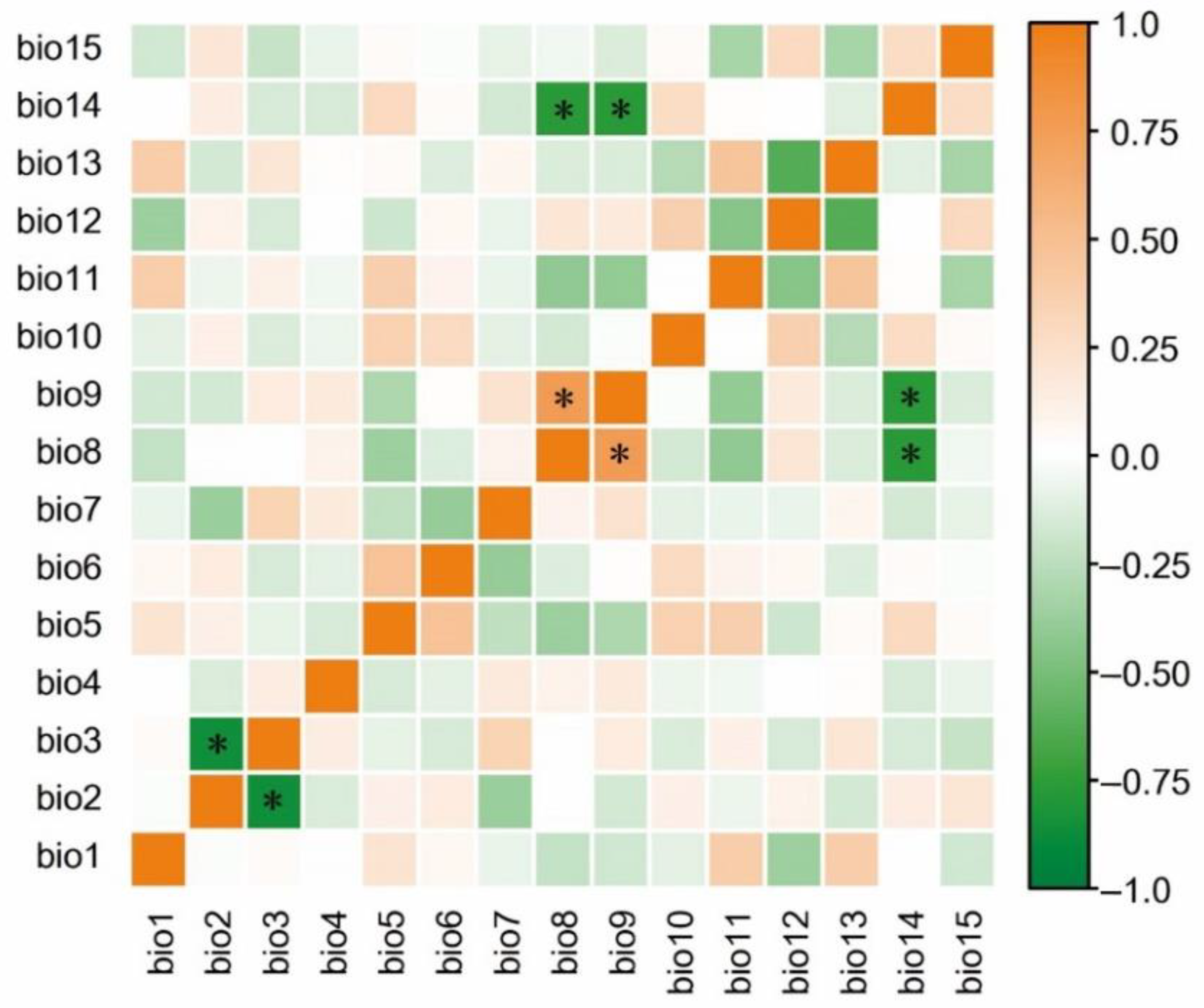
2.2.3. Collinearity Diagnosis of Environmental Variables

To avoid overfitting of the modeling results caused due to collinearity between environmental factors [42], this study first input all variables into the MaxEnt model to obtain preliminary simulation results and the contributions of each factor. Then, a Spearman rank correlation analysis of environmental factors was conducted [43] and those with low correlations (Spearman coefficient < 0.75) were screened out, combined with the contributions of each factor in the simulation results of all factors. Then, we considered the environmental conditions of geothermal samples used in this paper, excluding the factors with high correlation, low contribution and low impact [44] (Figure 3).

Finally, 12 variables were obtained (Figure 4).

2.3. Methods

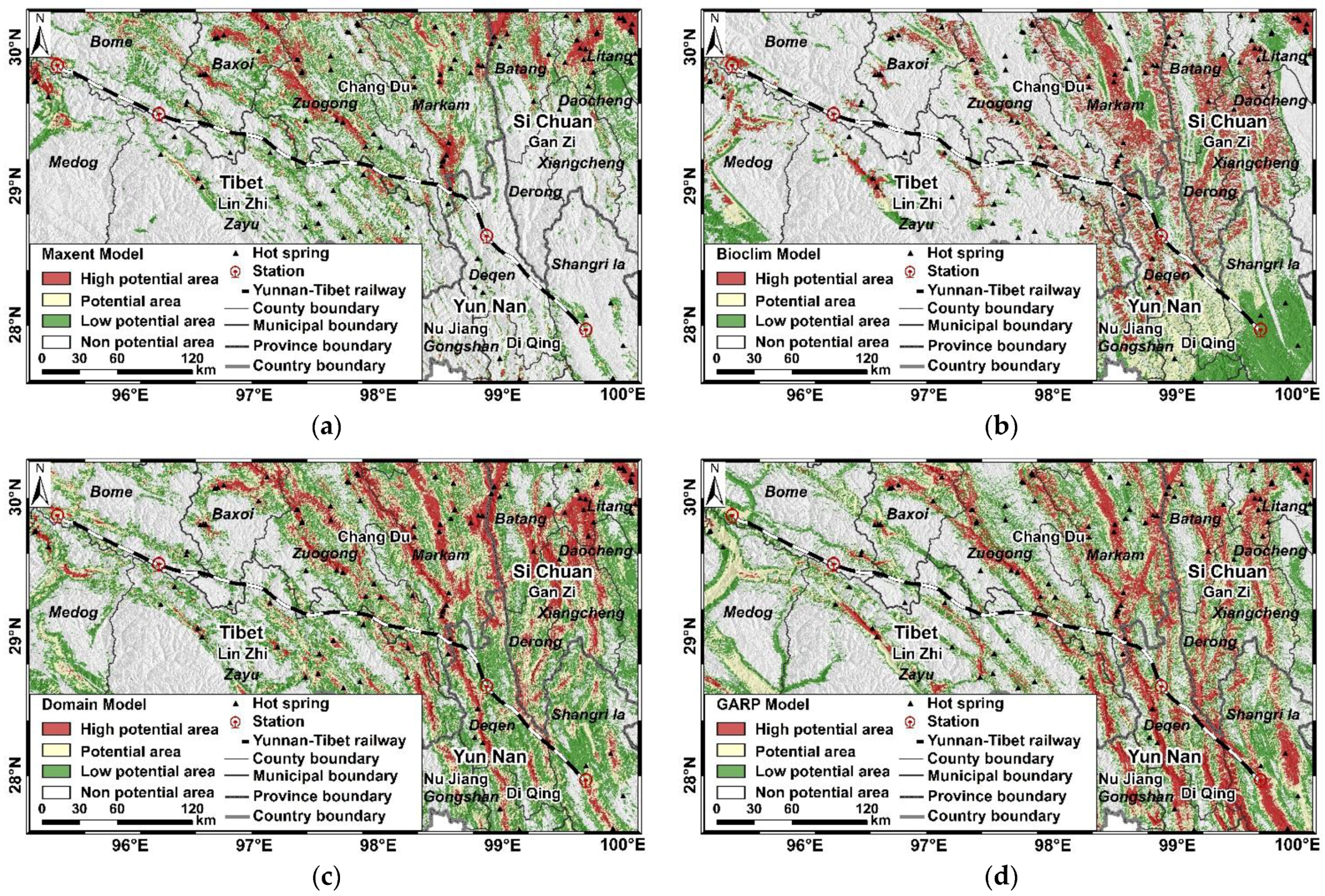
2.3.1. Prediction Models

Niche models were initially applied to the prediction and analysis of species distribution. In recent years, they have been widely used to predict the distribution and dynamics of landslides, debris flows, floods and other disasters [18]. When a niche model is applied to predict potential geothermal disaster areas, the known geothermal locations in the study area are considered to be equivalent to the known distribution of disaster locations, and environmental variables are used as prediction variables. At present, there are many commonly used niche models. Each can independently predict potentially vulnerable areas and each has a certain bias [21]. By using the idea of a set prediction system and integrating the prediction results of various models, the false-negative or false-positive effects caused by empirically selecting a model can be minimized [22,23]. Finally, the best model can be selected to predict potential geothermal disaster areas for analysis.

In recent years, the maximum entropy (MaxEnt) model has attracted extensive attention in the field of machine learning [16]. It simulates the geographical distribution of species based on correlations between environmental variables and the locations of target species [45]. The maximum entropy theory holds that, on the premise of meeting the existing conditions, the real state of the research object should be the state when the system entropy is maximal. That is, when predicting an unknown distribution according to known species locations and meeting the constraints of these samples, the real distribution of the target species in the study area is obtained when the unknown distribution entropy is maximal, to obtain the ecological environment distribution or climate suitability of the target species [46]. When the maximum entropy model is applied to the prediction of geothermal disasters, the known geothermal hot spring locations in the study area are equivalent to species locations, and the corresponding influences are the environmental variables of the model. The calculation formula is

$$H(\widehat{\pi })=-{\displaystyle {\displaystyle \sum }_{x\in \mathrm{X}}\stackrel{}{\widehat{\pi }(x)\cdot \ln }}\widehat{\pi }(x)$$

(8)

The unknown probability distribution is defined as $\widehat{\pi }$. For a finite element (X) in the study area, each element point (x) is assigned a non-negative probability, which sums to 1. The estimated probability distribution is $\widehat{\pi }$, and then H ($\widehat{\pi }$) is the entropy.

In this study, the MaxEnt model was used to simulate the distribution of geothermal disasters. Ten groups of training datasets and environmental variable datasets were used in the model. The maximum number of iterations was set to 500 and the maximum number of background points was 10,000. Weights were tested by the jack-knife method.

The Bioclim model is a framework model that extracts a limited range of environmental factors from known species distributions and then summarizes the environmental needs of the species into an “environmental envelope” [47]. By studying the climate parameters of the known distributions of species, the Bioclim model summarizes their ecological characteristics into a rectangular environmental envelope. Finally, many single envelopes form a group of environmental envelopes, which are then projected onto the target area. Each climate variable in the target area is compared with the environmental envelope system. If the position of a point in the envelope system space is within the environmental envelope, the model determines that the point is a potential distribution point [48]. The greater the number of species distribution points, the higher the accuracy of the model in predicting the suitable species habitat. However, due to the characteristics of the Bioclim model’s prediction process, when a species distribution presents a discrete trend, the predictions will contain errors, which will often overestimate the habitat range of the species.

The Domain model uses an environmental similarity matrix between points for simulation and prediction [49]. Its core idea is the Gower distance between points, which is the distance between two points in Euclidean geometric space. It was introduced into applied ecology to judge the similarity between a target area and a known distribution of a species. The Gower distance is treated by variance standardization or range standardization to ensure that its contribution in each dimension is the same. In the case of different samples, variance standardization can better avoid the error caused by it [50]. It only uses the existing species distribution and has a good effect when there are few predictive variables.

Based on the DIVA-GIS platform, this study simulated the potential distribution of geothermal disasters by importing 10 groups of training datasets and environmental variable datasets into the Bioclim and Domain models, respectively, in the Modeling module, and then made forecasts [50].

With the development of machine learning, a genetic algorithm for the rule set production (GARP) model was proposed. The operation principle of GARP is based on a regular genetic algorithm. During the operation of the model, the environmental factors affecting a species distribution are automatically selected, and all the selected factors are mapped to a certain area. Through superposition analysis, the non-random relationship between the known species distribution and study area is explored. The basic niche of the research target is determined and, finally, the potential geographical distribution of the research target is simulated and predicted [51,52]. In general, it uses the rule combination of the genetic algorithm to model the local environment and predict the species distribution [53]. It can well predict the suitable habitat of discrete species, which has advantages in this regard.

This study simulated the potential distribution of geothermal disasters based on the Desktop GARP platform. We imported 10 groups of training datasets and environmental variable datasets into the model, randomly created 10 repetitions, set the convergence limit to 0.01 and the maximum number of iterations to 1000 and, finally, added and stacked them in ArcGIS to obtain a predicted distribution map of geothermal disasters.

2.3.2. Test of Model Prediction Results

Using 10 groups of test sets obtained in the random segmentation step, the receiver operating characteristic (ROC) and kappa coefficient were calculated to verify the predictive accuracy of the model.

The area under the receiving operator curve (AUC) is the area covered by the ROC curve. The AUC value is not affected by the diagnostic threshold and is not sensitive to the incidence. At present, it is recognized as the best evaluation index and has been widely used in the accuracy evaluation of niche models. The numerical range of the AUC value distribution is 0–1, with higher values indicating a greater correlation between environmental variables and the distribution of simulated objects—that is, better simulation results. AUC values are considered to be “accurate” at 0.7–0.8, “very accurate” at 0.8–0.9 and “extremely accurate” > 0.9 [54].

The kappa coefficient is usually used to measure the consistency between simulation results and the real situation [55,56]. The distribution interval of the kappa coefficient is usually 0–1, with higher values indicating greater consistency between the simulation results and the real situation—that is, the more realistic the simulation is. The kappa coefficient is considered “moderate” at 0.4–0.6 and “significant” at >0.6 [57,58,59].

3. Result

3.1. Predicted Results of Models

From the 10 groups of prediction maps produced by each model, the map with the largest AUC was selected as the base map, and the potential areas of geothermal disaster were classified using the natural discontinuity classification method to obtain the maps of each model (Figure 5). The area of high geothermal disaster potential in the figure indicates that there is a high possibility of geothermal disasters in the area; a low potential area means that there is a low possibility of geothermal disasters in the area; a non-potential area means that there is no geothermal disaster potential in the area. From the classification chart of the prediction potential and statistical results, it can be seen that the distribution trends predicted by the four models are relatively close, but the areas and specific details are different. The predicted distribution map of the MaxEnt model (Figure 5) shows that the area with high potential for geothermal disaster is the smallest, and is mainly distributed in Eastern Tibet and Western Sichuan at 29–31°N, being mainly concentrated in the north of Medog County, Zayu County, the east of Bome County, Nyingchi City, Tibet Autonomous Region, the south and east of Markam County, Qamdo City, the south and west of Zuogong County and the east of Baxoi County, the northwest of Deqen County, Diqing Tibetan Autonomous Prefecture, Yunnan Province, the west of Batang County and southwest of Litang County, Garze Tibetan Autonomous Prefecture and Sichuan Province. The predicted distribution map of the Bioclim model (Figure 5) shows that the high potential areas of geothermal disaster are mainly distributed in Eastern Tibet, Western Sichuan and Northwest Yunnan at 28–31°N and 97–100°E, mainly in the north of Medog County, Nyingchi City, the northeast of Zayu County, the southwest of Bome County, Markam County, Zuogong County, the east and west of Qamdo City and the east of Baxoi County; Northwest of Deqen County, Diqing Tibetan Autonomous Prefecture, Yunnan Province; the west and east of Batang County, Garze Tibetan Autonomous Prefecture, Sichuan Province, the south of Litang County, Xiangcheng County and Derong County. The predicted distribution map of the Domain model (Figure 5) shows that the high potential areas of geothermal disaster are mainly distributed in Eastern Tibet, Western Sichuan and Northwest Yunnan at 28–31°N and 97–100°E, mainly in the north of Medog County, Nyingchi City, the east of Zayu County, Markam County, Zuogong County, the east and west of Qamdo city and the east of Baxoi County, Tibet Autonomous Region; Deqen County, Diqing Tibetan Autonomous Prefecture, Yunnan Province; the west and east of Batang County, Garze Tibetan Autonomous Prefecture, Sichuan Province, the south of Litang County, the southwest of Xiangcheng County and Derong County. The predicted distribution map of the GARP model (Figure 5) shows that the geothermal disaster and high potential area is the largest, which is mainly distributed in Eastern Tibet, Western Sichuan and Northwest Yunnan at 28–31°N and 97–100°E, mainly in the northeast of Zayu County, Nyingchi City, Tibet Autonomous Region, Markam County, Zuogong County, Eastern and Western Qamdo City and Eastern Baxoi County; Deqen County and Shangri La County, Diqing Tibetan Autonomous Prefecture, Yunnan Province; the west and east of Batang County, Garze Tibetan Autonomous Prefecture, Sichuan Province, the south of Litang County, Xiangcheng County and Derong County.

Although the geothermal sample data and environmental variables selected by each model are the same, there are great differences in the results predicted by different niche models on the distribution of potential areas of geothermal disaster [60,61]. The predicted differences are mainly reflected in the junction areas of the Southeast Tibet Autonomous Region, Northwest Yunnan Province and Southwest Sichuan Province. This is mainly caused by the different algorithms used by each model. The area predicted by the MaxEnt model is the smallest, but it is more clear at the local level of detail because the MaxEnt model algorithm infers the environmental demand of geothermal disasters and simulates their distribution based on the principle of maximum entropy. It focuses on eliminating the commission in the simulation [62]. During its operation, the entropy increases with the input of environmental variables associated with each set of geothermal sample data and the number of iterations. The research results tend to the real niche [63]; that is, under the real conditions, the distribution range of geothermal disasters, and the prediction results, are more delicate. The area predicted by the GARP model is large and the overall performance is good because GARP uses a genetic algorithm. It searches the environmental variables related to the research samples and selects the optimal rule set to predict the distribution area of geothermal disasters. It focuses on eliminating the omission error in the simulation; that is, the selection of the optimal model is based on the minimum omission rate, and the research results are biased towards the basic niche [64]. That is, in the ideal state without interference, the maximum distribution range that may be occupied by geothermal disasters [65], which is predicted to expand the range of geothermal disaster area, and the MaxEnt model algorithm can achieve a good trade-off between omission rate and recording error rate. The prediction ranges of the Bioclim and Domain models are between those of MaxEnt and GARP because the Bioclim model is based on the principle of the environmental envelope and the Domain model uses the Gower algorithm. They are greatly affected by the geothermal sample points. Geothermal sample distribution data mainly come from field survey mapping. The sample data have a certain preference, so researchers generally take samples according to their research needs or simply collect data for different work areas. The sample information is scattered and is not systematic and representative. Secondly, fewer geothermal sample data may lead to a reduction in the niche space and, due to the complex geological and climatic conditions in some areas, the niches of geothermal hotspots in different regions may drift [66]. Therefore, different models have their advantages and disadvantages. They can refer to each other, be comprehensively compared and an appropriate prediction result can be selected.

3.2. Evaluation of the Predictive Accuracy of Different Models

In this paper, 10 groups of training data and test data were used to analyze the ROC curve and conduct kappa consistency tests of the four models (Figure 6).

The average AUC of the MaxEnt model was 0.842, indicating a high correlation between 12 environmental variables and the distribution of geothermal sample points. Hence, the prediction results are very accurate. The average AUC of the Bioclim model is 0.693, indicating that the correlation between environmental variables and the distribution of simulated objects is general, and the prediction results are general. The average AUC of the Domain model is 0.822, which shows that there is a great correlation between 12 environmental variables and the distribution of geothermal sample points; hence, the predictions are very accurate. The average AUC of the GARP model is 0.783 (

Table 2. AUC and kappa values of the four models.

The Area	The Area under Receiver Operating CharacteristicCurve (AUC)				Consistency Test Statistics (Kappa)
	MaxEnt	Bioclim	Domain	GARP	MaxEnt	Bioclim	Domain	GARP
1	0.894	0.730	0.872	0.814	0.707	0.452	0.628	0.605
2	0.839	0.699	0.787	0.766	0.621	0.371	0.441	0.485
3	0.848	0.754	0.811	0.768	0.586	0.436	0.560	0.490
4	0.821	0.586	0.787	0.780	0.534	0.271	0.546	0.449
5	0.868	0.763	0.835	0.820	0.698	0.525	0.592	0.570
6	0.825	0.718	0.807	0.782	0.576	0.417	0.519	0.544
7	0.795	0.654	0.786	0.750	0.579	0.366	0.460	0.490
8	0.860	0.696	0.868	0.811	0.706	0.408	0.628	0.645
9	0.810	0.597	0.823	0.754	0.567	0.316	0.531	0.453
10	0.861	0.733	0.845	0.787	0.629	0.466	0.615	0.512
Average	0.842	0.693	0.822	0.783	0.620	0.403	0.552	0.524

), indicating that there is a strong correlation between 12 environmental variables and the distribution of geothermal sample points; hence, the predicted results are more accurate. The average AUC of the four models is higher than that of the random model (AUC = 0.5), indicating that the four models have good geothermal disaster prediction effects, with the average AUC of the MaxEnt model being the largest.

By analyzing the kappa values of the four models, it can be seen that the average of the MaxEnt model is 0.620, and those of the Bioclim, Domain and GARP models are 0.403, 0.552 and 0.524, respectively, indicating that the consistency of the MaxEnt model is significant, while those of the other three models are moderate, and they can be used to predict the potential geothermal disaster areas. It can be seen from Figure 6 that the average AUC and average kappa values of the MaxEnt and Domain models are high and have good consistency, with those of the MaxEnt model being slightly higher. Therefore, the MaxEnt model is the best model for predicting the potential distribution of geothermal disasters.

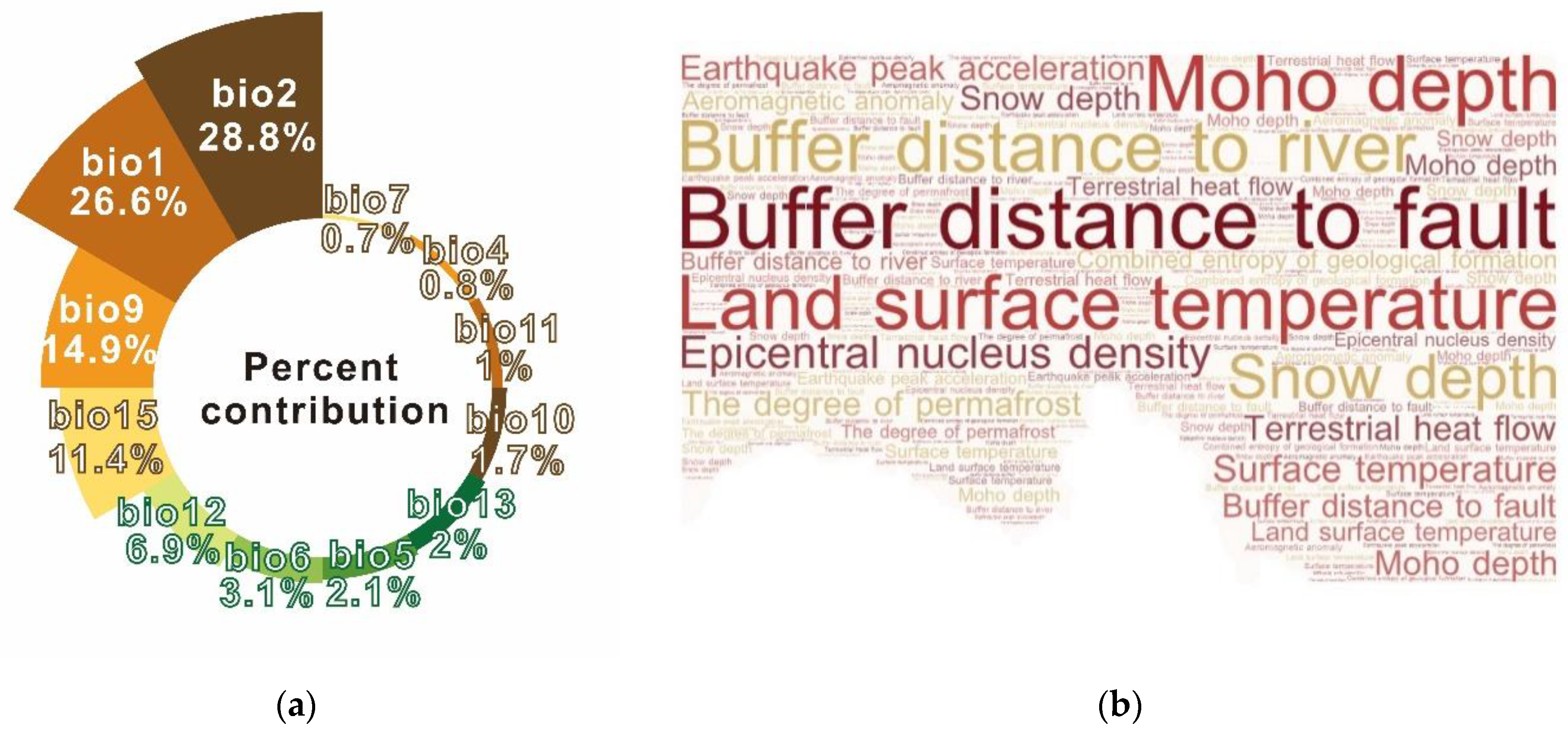
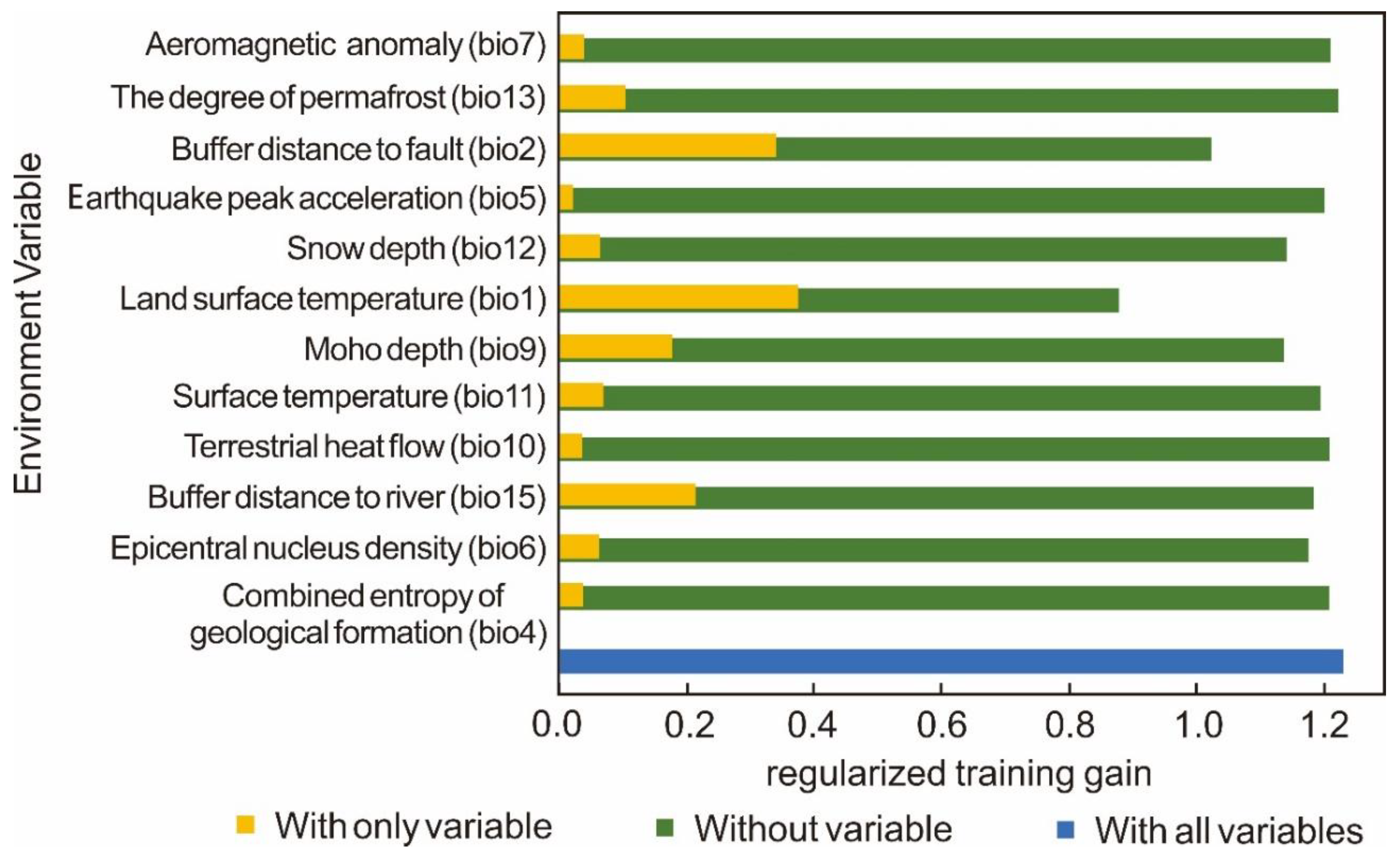
3.3. Analysis of Environmental Variables Affecting the Potential Geothermal Disaster Area

The percentage contribution of each environmental variable to the prediction of the distribution of potential areas of geothermal disaster risk is shown in Figure 7. Among the 12 environmental variables in the word cloud diagram (Figure 7), the fault buffer distance (bio 2) has the greatest contribution, while the LST (bio 1), water buffer distance (bio 9) and Moho depth (bio 15) also have great impacts on the distribution of geothermal disasters.

From the jack-knife test results (Figure 8), the contribution rate of each environmental variable to the distribution of geothermal disaster potential areas can be obtained. The yellow bar represents the contribution of each environmental factor to the risk probability distribution when the interference of other factors is removed, and its length represents the contribution rate. The green bar corresponding to each environmental factor represents the total contribution rate of all other variables (except this factor), and the sum of the cumulative contribution rates of all environmental variables is represented by the blue bar at the bottom. From Figure 8, it can be seen that when only a single environmental factor is used, the four factors that have the greatest impact on the normalization training gain are LST, fault buffer distance, river buffer distance and Moho depth.

From the combination of the two, it can be concluded that the LST, fault buffer distance, river buffer distance and Moho depth are the most important environmental variables that lead to the distribution of geothermal disasters along the Yunnan–Tibet railway project. The higher the LST, the closer it is to an active fault and river, and the deeper the Moho depth, the more prone it is to geothermal disaster. The line passage in this area should be fully considered in the planning and design of the railway project.

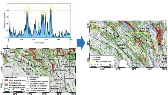
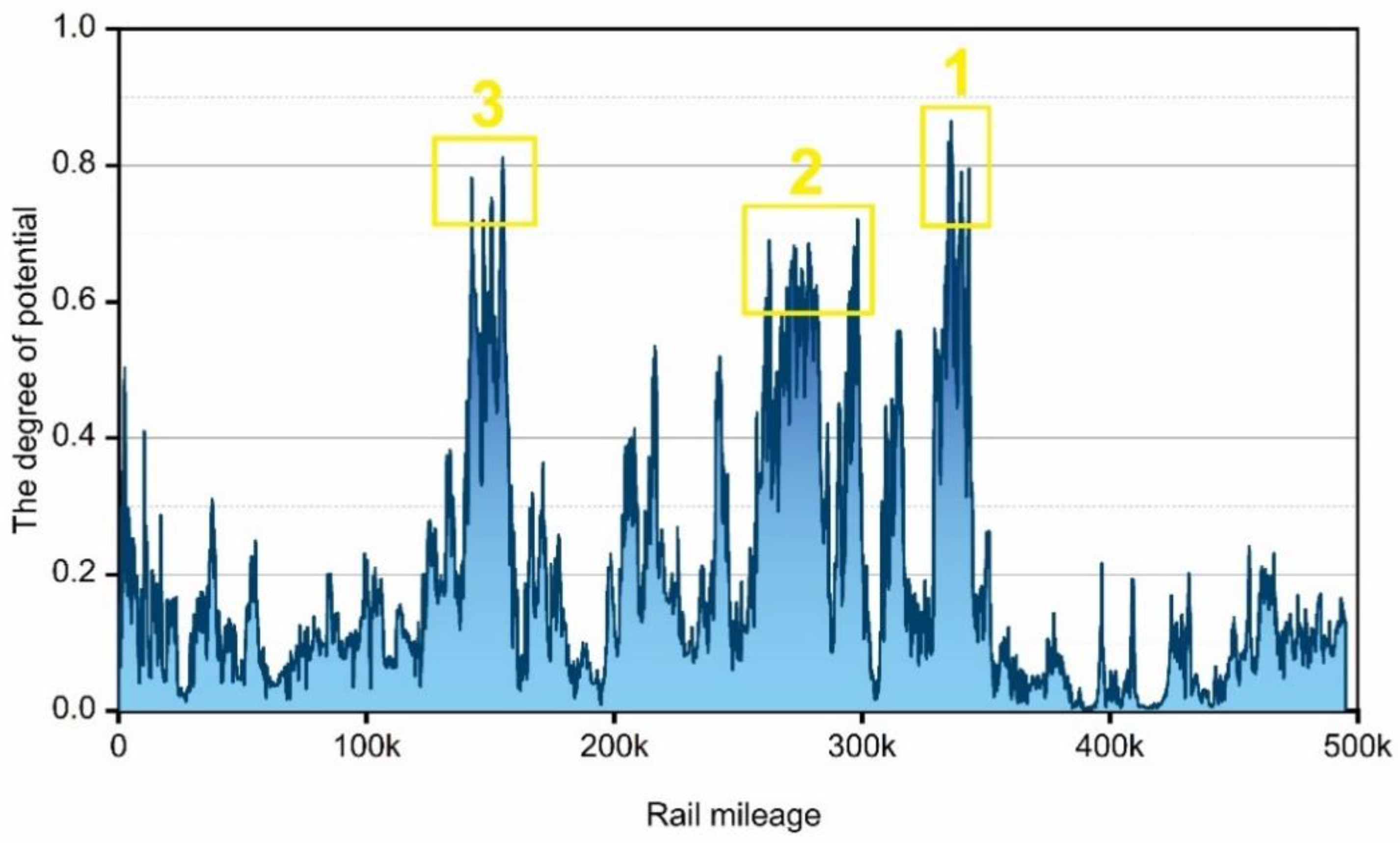
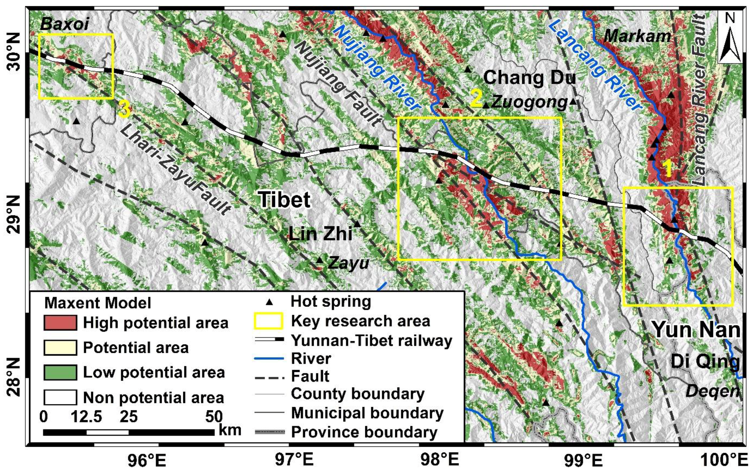
3.4. Analysis of Key Areas of Geothermal Disaster along Yunnan–Tibet Railway

By overlaying the prediction results of the MaxEnt model of the Yunnan–Tibet railway line in ArcGIS (Figure 9), the key areas of geothermal disasters were delineated (Figure 10). It is found that the railway passes through three key areas of geothermal disaster. (1) Markam-Deqen, distributed at the junction of Eastern Tibet and Northwestern Yunnan at 28°53′N and 98°37′E. Specifically, it is located in a canyon area where the Lancang River flows at the junction of the south of Markam County, Qamdo City, Tibet Autonomous Region and the north of Deqen County, Diqing Tibetan Autonomous Prefecture, Yunnan Province. It is approximately 1500–4000 m above sea level, runs north–south, is nearly vertically distributed with the Lancang River Fault Zone and is located in the docking zone between the Gondwana plate and South China plate. There are many high-temperature hot springs, making it the second-largest key area along the Yunnan–Tibet railway. (2) Zuogong-Zayu, distributed in Eastern Tibet at 29°18′N and 98°10′E. It is specifically located in the canyon zone at the junction of the south of Zuogong County, Qamdo City, Tibet Autonomous Region and the north of Zayu County, Nyingchi City. It is approximately 2000–5000 m above sea level and runs northwest–southeast. Nujiang River flows through it and it is distributed nearly parallel to the Nujiang fault zone. It is located in the block docking zone between the Tengchong block and Baoshan block of the Gondwana plate. There are many high-temperature hot springs, and it is the largest key area along the Yunnan–Tibet railway. (3) Baxoi-Zayu, distributed in Eastern Tibet at 29°20′N and 96°55′E. It is located at the junction of the southeast of Baxoi County, Qamdo City, Tibet Autonomous Region and the north of Zayu County, Nyingchi City, with an altitude of around 4500–5000 m. It is northwest–southeast trending and distributed nearly parallel to the Lhari-Zayu fault zone, which is controlled by the east direction of the Qinghai–Tibet Plateau and the clockwise rotation around the East Himalayan tectonic knot. Since the Holocene, it has had strong activity, mainly dextral strike-slips [60], and this area is the smallest key area along the Yunnan–Tibet railway. For the key areas of geothermal disaster, the railway route should follow the disaster reduction principle of avoiding around first, and then passing through the low potential area or non-potential area quickly in a short distance based on finding out the distribution characteristics of geothermal anomalies [26].

4. Discussion

Based on Landsat-8 images and niche models, this paper forecast potential areas of geothermal disaster along the Yunnan–Tibet railway project. Although the geothermal data and environmental variables used in each model were the same, there are some differences in their predictions of potential geothermal disaster areas. The prediction differences mainly occur in the border areas of the Southeast Tibet Autonomous Region, Northwest Yunnan Province and Southwest Sichuan Province, which is mainly due to the different algorithms used in each model. The four niche models (MaxEnt, Bioclim, Domain and GARP) used in this study each have their own advantages. They use the known distribution data of geothermal samples and environmental variables caused by geothermal disasters to build models according to different algorithm operations. Each model is screened 10 times to find the best model prediction results. The analysis of the ROC curve and kappa coefficient shows that the four models have good geothermal disaster prediction effects. Among them, the average AUC and kappa coefficients of the MaxEnt model are the largest and the accuracy is the highest. Finally, combining the preferences of different model algorithms, ROC curve and kappa coefficient, it is concluded that the MaxEnt model is the best at predicting the potential distribution of geothermal disasters. The MaxEnt prediction results were selected as the final results, but the fitting degree of geothermal disasters is high. When other geological disasters are replaced, the results may be different. Therefore, when predicting the potential area of a geological disaster, multiple models should be used and the best one selected. At present, most studies choose potential area analysis without model screening. Due to the uncertainty in model prediction, the results are unstable, so the combination of multiple models will improve the reliability and stability of the results. At the same time, this study also has problems that need to be improved; that is, too many environmental variables will affect the prediction results.

The terrain along the Yunnan–Tibet railway project is difficult and dangerous, and the area covered by ice and snow is large, making it very difficult to carry out conventional large-area ground geothermal surveys. Through Landsat-8 satellite images, using the advantages of the large amount of information provided by thermal infrared remote sensing, and its high monitoring accuracy and lack of restriction by ground conditions, we can effectively perceive ground temperature anomalies in the study area. Based on the mechanism of spatial information acquisition and analysis, as an important part of Earth big data, Earth observation data and other means can quickly, accurately and macroscopically reflect the key information such as the spatial location of high-temperature heat disaster causing factors, and play a basic role in the construction of plateau railway engineering. At the same time, this study can provide a reference for the planning and construction of railway projects in the geothermal zones of other countries with complex topographic and geological conditions and difficulty in ground geothermal investigation.

Environmental variables are closely related to the spatial distribution of geothermal sampling points. Combined with the contribution rate of environmental variables and the test results of the jack-knife test, the LST, fault buffer distance, river buffer distance and Moho depth were found to be the most important predictors of the distribution of geothermal disasters along the Yunnan–Tibet railway project. The higher the LST, the closer the area is to an active fault and river. The deeper the Moho depth, the more prone the area is to geothermal disasters. Railway engineers should fully consider the line’s passage through these areas.

According to the results of the MaxEnt model, the high geothermal disaster potential areas in the study area are mainly distributed in Eastern Tibet and Western Sichuan at 29–31°N, mainly in the north of Medog County, Zayu County, the east of Bome County, Nyingchi City, Tibet Autonomous Region, the South and east of Markam County, Qamdo City, the south and west of Zuogong county and the east of Baxoi County; northwest of Deqen County, Diqing Tibetan Autonomous Prefecture, Yunnan Province; west of Batang County and southwest of Litang County, Garze Tibetan Autonomous Prefecture, Sichuan Province. Among them, there are three key areas of geothermal disaster along the Yunnan–Tibet railway project, namely Markam-Deqen, Zuogong-Zayu and Baxoi-Zayu. The LSTs in these three key areas are high and there are active fault zones and a large number of geothermal hot springs in these areas. Among them, Lancang River and Nujiang River flow through the Markam-Deqen and Zuogong-Zayu areas, respectively, and there are many disaster-causing factors. For the key geothermal disaster areas, the railway route selection should follow the disaster reduction principle of avoiding first and then passing through low or no-risk areas quickly over short distances based on finding out the distribution characteristics of geothermal anomalies.

5. Conclusions

The United Nations industry, innovation and infrastructure goal (SDG 9) emphasizes the construction of disaster-resilient infrastructure. The sustainable cities and communities goal (SDG 11) calls for the building of inclusive, safe, disaster-resilient and sustainable cities and human settlements. Therefore, infrastructure such as railways plays a vital role in achieving the SDG goals.

The Yunnan–Tibet railway is located in the parallel flow area of Hengduanshan and three rivers in China. The internal and external dynamic geological processes are significant, and there are unfavorable geological conditions such as high tectonic stresses, strong earthquakes, active faults, gravity unfavorable geology and thermally altered rock masses, which pose great challenges to railway route selection. Therefore, the route selection in the survey section should not only follow the principles of “topographic route selection” and “geological route selection”, but also reduce the impact of geological disasters on railway engineering from the source, and implement the concept of “disaster reduction and route selection” of natural disasters on the risk regulation of the railway life cycle. In this paper, four niche models were introduced into the project disaster prediction to predict the geothermal disaster potential areas along the Yunnan–Tibet railway project, and good results were obtained. However, the use of 12 environmental variables will affect the uncertainty of the results, so it should still be fully considered in future research. The next work will aim to systematically analyze the predicted high potential area in combination with geothermal theory and engineering theory, discuss the causes and impacts of geothermal disasters in this area, guide railway route selection and provide a scientific basis and technical support for the project planning, route optimization and sustainable development of the Yunnan–Tibet railway. This study also provides a reference for the planning and construction of railway projects in geothermal zones in other countries with complex topographic and geological conditions and great difficulty in ground geothermal investigation.

References

1. Wang, J. Research on Main Engineering Geological Problems and Principles of Geological Route Selection for Yunnan-Tibet Railway. Railw. Stand. Des. 2021, 65, 7–13. [Google Scholar] [CrossRef]
2. Liu, Z. Analysis and Prediction of Geothermal Characteristics of Sanbaishan Tunnel. J. Railw. Sci. Eng. 2022, 19, 1364–1373. [Google Scholar] [CrossRef]
3. Wang, X.; Huang, R.; Huang, G. Analysis of Effects of Groundwater Geotemperature Anomaly in Deeply Lying Longon and Big Tunnel. J. Geol. Hazards Environ. Preserv. 1996, 7, 24–28. [Google Scholar]
4. Guo, H.; Chen, F.; Sun, Z.; Liu, J.; Liang, D. Big Earth Data: A Practice of Sustainability Science to Achieve the Sustainable Development Goals. Sci. Bull. 2021, 66, 1050–1053. [Google Scholar] [CrossRef]
5. Guo, H.; Liang, D.; Chen, F.; Sun, Z.; Liu, J. Big Earth Data Facilitates Sustainable Development Goals. Bull. Chin. Acad. Sci. 2021, 36, 874–884. [Google Scholar] [CrossRef]
6. Yan, J.; He, C.; Zeng, Y.; Wang, B.; Zhang, J. Cooling Technology and Effect Analysis for High Geothermal Tunnel on Sichuan-Tibet Railway. China Railw. Sci. 2019, 40, 53–62. [Google Scholar] [CrossRef]
7. Luo, F.; Du, S.; Meng, X.; Zhang, Z.; Dong, Q.; Hao, L.; Zhang, W.; Huang, Y.; Zhang, X.; Wang, Y. Research on the “Space-Aero-Ground” Remote Sensing Geological Survey Technology of Sichuan-Tibet Railway. J. Railw. Eng. Soc. 2021, 38, 1–7. [Google Scholar]
8. Gruber, S.; Haeberli, W. Permafrost in Steep Bedrock Slopes and Its Temperature-Related Destabilization Following Climate Change. J. Geophys. Res. 2007, 112, F02S18. [Google Scholar] [CrossRef] [Green Version]
9. Isaksen, K.; Sollid, J.L.; Holmlund, P.; Harris, C. Recent Warming of Mountain Permafrost in Svalbard and Scandinavia. J. Geophys. Res. 2007, 112, F02S04. [Google Scholar] [CrossRef]
10. Liu, G.; Zhao, L.; Xie, C.; Pang, Q.; Du, E.; Qiao, Y. Variation Characteristics and Impact Factors of the Depth of Zero Annual Amplitude of Ground Temperature in Permafrost Regions on the Tibetan Plateau. J. Glaciol. Geocryol. 2016, 38, 1189–1200. [Google Scholar] [CrossRef]
11. Zhang, N.; Zhang, W.; Li, L.; Lan, H. Geothermal Characteristics of Qinghai-Tibet Plateau and Risk Analysis of Deep Underground Geothermal Hazards for Major Linear Sichuan-Tibet Railway Project. J. Eng. Geol. 2021, 29, 326–341. [Google Scholar] [CrossRef]
12. Chen, Z.; Chang, R.; Zhao, W.; Li, S.; Guo, H.; Xiao, K.; Wu, L.; Hou, D.; Zou, L. Quantitative Prediction and Evaluation of Geothermal Resource Areas in the Southwest Section of the Mid-Spine Belt of Beautiful China. Int. J. Digit. Earth 2022, 15, 748–769. [Google Scholar] [CrossRef]
13. Xiao, K.; Xiang, J.; Fan, M.; Xu, Y. 3D Mineral Prospectivity Mapping Based on Deep Metallogenic Prediction Theory: A Case Study of the Lala Copper Mine, Sichuan, China. J. Earth Sci. 2021, 32, 348–357. [Google Scholar] [CrossRef]
14. Chen, J.; Xiang, J.; Hu, Q.; Yang, W.; Lai, Z.; Hu, B.; Wei, W. Quantitative Geoscience and Geological Big Data Development: A Review. Acta Geol. Sin. English Ed. 2016, 90, 1490–1515. [Google Scholar] [CrossRef]
15. Zhang, S.; Carranza, E.J.M.; Xiao, K.; Wei, H.; Yang, F.; Chen, Z.; Li, N.; Xiang, J. Mineral Prospectivity Mapping Based on Isolation Forest and Random Forest: Implication for the Existence of Spatial Signature of Mineralization in Outliers. Nat. Resour. Res. 2021, 1–9. [Google Scholar] [CrossRef]
16. Zhang, S.; Xiao, K.; Carranza, E.J.M.; Yang, F. Maximum Entropy and Random Forest Modeling of Mineral Potential: Analysis of Gold Prospectivity in the Hezuo–Meiwu District, West Qinling Orogen, China. Nat. Resour. Res. 2019, 28, 645–664. [Google Scholar] [CrossRef]
17. Abuzied, S.M.; Kaiser, M.F.; Shendi, E.A.H.; Abdel-Fattah, M.I. Multi-Criteria Decision Support for Geothermal Resources Exploration Based on Remote Sensing, GIS and Geophysical Techniques along the Gulf of Suez Coastal Area, Egypt. Geothermics 2020, 88, 101893. [Google Scholar] [CrossRef]
18. Abdel-Fattah, M.I.; Shendi, E.A.H.; Kaiser, M.F.; Abuzied, S.M. Unveiling Geothermal Potential Sites along Gulf of Suez (Egypt) Using an Integrated Geoscience Approach. Terra Nova 2021, 33, 306–319. [Google Scholar] [CrossRef]
19. Zhao, W.; Dong, Q.; Chen, Z.; Feng, T.; Wang, D.; Jiang, L.; Du, S.; Zhang, X.; Meng, D.; Bian, M.; et al. Weighted Information Models for the Quantitative Prediction and Evaluation of the Geothermal Anomaly Area in the Plateau: A Case Study of the Sichuan–Tibet Railway. Remote Sens. 2021, 13, 1606. [Google Scholar] [CrossRef]
20. Gengping, Z.; Guoqing, L.; Wenjun, B.; Yubao, G. Ecological Niche Modeling and Its Applications in Biodiversity Conservation. Biodivers. Sci. 2013, 21, 90–98. [Google Scholar] [CrossRef]
21. Araujo, M.; New, M. Ensemble Forecasting of Species Distributions. Trends Ecol. Evol. 2007, 22, 42–47. [Google Scholar] [CrossRef] [PubMed]
22. Wang, G.; Gen, Q.; Xiao, M.; Zhang, M.; Zhang, Y.; Wang, Z. Predicting Pseudolarix Amabilis Potential Habitat Based on Four Niche Models. Acta Ecol. Sin. 2020, 40, 6096–6104. [Google Scholar] [CrossRef]
23. Zhang, Q.; Zhang, D.F.; Wu, M.L.; Guo, J.; Sun, C.Z.; Xie, C.X. Predicting the Global Areas for Potential Distribution of Gastrodia Elata Based on Ecological Niche Models. Chin. J. Plant Ecol. 2017, 41, 770–778. [Google Scholar] [CrossRef]
24. Ming, Q. A Study on The Neotectonic Division & Environment Evolution of Qing-Zang Plateau & Three Parallel Rivers area. Yunnan Geol. 2007, 4, 387–396. [Google Scholar] [CrossRef]
25. Zheng, Y.; Yang, Y.; Jiang, L. The Particularity of Engineering Geology on Yunnan-Tibet Route in Glacier Snowfield Area. J. Railw. Eng. Soc. 2005, A1, 216–221. [Google Scholar] [CrossRef]
26. Song, Z.; Zhu, Y.; Wei, Y.; Jiang, L.; Zhang, G. Research on the Engineering Geological Hazards-Reduction Route Selection in Three Parallel Rivers Regions for the Yunnan-Tibet Railway. J. Railw. Eng. Soc. 2019, 36, 1–6. [Google Scholar]
27. Zhang, J.; Zhang, Y.; Qu, Y.; Cao, H. In Depth Discussions on The Engineering Geological Problems Along Sanjiang Sector of Yunan-Tibet Railway Line. J. Eng. Geol. 2010, 18, 781–789. [Google Scholar] [CrossRef]
28. Liu, A.; Zheng, J.; Li, J.; Du, J.; Li, F. Comparison Study on Resource Evaluation Methods of Shallow Geothermal Energy and Traditional Geothermal Energy. Urban Geol. 2018, 13, 37–41. [Google Scholar] [CrossRef]
29. Zhang, L.; Li, G. Shallow Geothermal Resources. West. Resour. 2019, 1, 178–180. [Google Scholar] [CrossRef]
30. Wang, X.; Huang, R. Evaluation and Prediction of Temperature Field in Deep Buried Long Tunnel. Hydrogeol. Eng. Geol. 1996, 23, 6–10. [Google Scholar]
31. Chen, Z.; Qing, D.; Chen, J.; Zhao, W.; Jiang, L.; Zhang, G.; Feng, T.; Wang, D.; Bi, X.; Bian, M.; et al. Research on Quantitative Prediction and Evaluation of Geo- Thermal Anomaly Area in Qamdo-Nyingchi Section of Sichuan-Tibet Railway. Remote Sens. Technol. Appl. 2021, 36, 1368–1378. [Google Scholar] [CrossRef]
32. Revil, A.; Pezard, P.A. Streaming Electrical Potential Anomaly along Faults in Geothermal Areas. Geophys. Res. Lett. 1998, 25, 3197–3200. [Google Scholar] [CrossRef]
33. Xiao, K.; Pirajno, F.; Xu, Y.; Zhang, S.; Sun, L.; Cong, Y.; Fan, J.; Yin, J.; Zhu, Y.; Wei, H. Study on the Major Minerals Potential in China. Ore Geol. Rev. 2020, 127, 103816. [Google Scholar] [CrossRef]
34. Bayrak, Y.; Bayrak, E. Regional Variations and Correlations of Gutenberge-Richter Parameters and Fractal Dimension for the Different Seismogenic Zones in Western Anatolia. J. Asian Earth Sci. 2012, 58, 98–107. [Google Scholar] [CrossRef]
35. Aydogan, D. Extraction of Lineaments from Gravity Anomaly Maps Using the Gradient Calculation: Application to Central Anatolia. Earth Planets Sp. 2011, 63, 903–913. [Google Scholar] [CrossRef] [Green Version]
36. Wang, D.F. Aeromagnetic Series Maps and Specifications of Qinghai—Tibet Plateau and Adjacent Areas; Geological Publishing House: Beijing, China, 2013. [Google Scholar]
37. Qiu, N.; Tang, B.; Zhu, C. Deep Thermal Background of Hot Spring Distribution in the Chinese Continent. Acta Geol. Sin. 2022, 96, 195–207. [Google Scholar] [CrossRef]
38. Fang, S.; Mao, K.; Xia, X.; Wang, P.; Shi, J.; Bateni, S.M.; Xu, T.; Cao, M.; Heggy, E.; Qin, Z. Dataset of Daily Near-Surface Air Temperature in China from 1979 to 2018. Earth Syst. Sci. Data 2022, 14, 1413–1432. [Google Scholar] [CrossRef]
39. Zou, D.; Zhao, L.; Sheng, Y.; Chen, J.; Hu, G.; Wu, T.; Wu, J.; Xie, C.; Wu, X.; Pang, Q.; et al. A New Map of Permafrost Distribution on the Tibetan Plateau. Cryosph 2017, 11, 2527–2542. [Google Scholar] [CrossRef] [Green Version]
40. Yan, D.; Ma, N.; Zhang, Y. Development of a Fine-Resolution Snow Depth Product Based on the Snow Cover Probability for the Tibetan Plateau: Validation and Spatial–temporal Analyses. J. Hydrol. 2022, 604, 127027. [Google Scholar] [CrossRef]
41. Wang, J.; Wang, J.; Ye, H. An Interpolated Temperature and Precipitation Dataset at 1-Km Grid Resolution in China (2000–2012). China Sci. Data 2017, 2, 88–95. [Google Scholar] [CrossRef]
42. Graham, M.H. Confronting Multicollinearity in Ecological Multiple Regression. Ecology 2003, 84, 809–2815. [Google Scholar] [CrossRef] [Green Version]
43. Zhang, M.G.; Slik, J.W.F.; Ma, K.P. Using Species Distribution Modeling to Delineate the Botanical Richness Patterns and Phytogeographical Regions of China. Sci. Rep. 2016, 6, 22400. [Google Scholar] [CrossRef] [PubMed] [Green Version]
44. Mai, J.; Xian, Y.; Liu, G. Predicting Potential Rainfall-Triggered Landslides Sites in Guangdong Province (China) Using MaxEnt Model under Climate Changes Scenarios. J. Geo Inf. Sci. 2021, 23, 2042–2054. [Google Scholar] [CrossRef]
45. Franklin, J.; Davis, F.W.; Ikegami, M.; Syphard, A.D.; Flint, L.E.; Flint, A.L.; Hannah, L. Modeling Plant Species Distributions under Future Climates: How Fine Scale Do Climate Projections Need to Be? Glob. Chang. Biol. 2013, 19, 473–483. [Google Scholar] [CrossRef] [PubMed] [Green Version]
46. Phillips, S.J.; Anderson, R.P.; Schapire, R.E. Maximum Entropy Modeling of Species Geographic Distributions. Ecol. Model. 2006, 190, 231–259. [Google Scholar] [CrossRef] [Green Version]
47. Booth, T.H.; Nix, H.A.; Busby, J.R.; Hutchinson, M.F. Bioclim: The First Species Distribution Modelling Package, Its Early Applications and Relevance to Most Current MaxEnt Studies. Divers. Distrib. 2014, 20, 1–9. [Google Scholar] [CrossRef]
48. Busby, J.R. BIOCLIM—A Bioclimate Analysis and Prediction System. Nat. Conserv. Cost Eff. Biol. Surv. Data Anal. 1991, 6, 8–9. [Google Scholar]
49. Guisan, A.; Zimmermann, N.E. Predictive Habitat Distribution Models in Ecology. Ecol. Model. 2000, 135, 147–186. [Google Scholar] [CrossRef]
50. Yunsheng, W. Application of ROC Curve Analysis in Evaluating the Performance of Alien Species’ Potential Distribution Models. Biodivers. Sci. 2007, 15, 365. [Google Scholar] [CrossRef]
51. Higgins, S.I.; Richardson, D.M.; Cowling, R.M. Modeling Invasive Plant Spread: The Role of Plant-Environment Interactions and Model Structure. Ecology 1996, 77, 2043–2054. [Google Scholar] [CrossRef]
52. Higgins, S.I.; Richardson, D.M.; Cowling, R.M.; Trinder-Smith, T.H. Predicting the Landscape-Scale Distribution of Alien Plants and Their Threat to Plant Diversity. Conserv. Biol. 1999, 13, 303–313. [Google Scholar] [CrossRef]
53. Stockwell, D.; Peters, D. The GARP Modelling System: Problems and Solutions to Automated Spatial Prediction. Int. J. Geogr. Inf. Sci. 1999, 13, 143–158. [Google Scholar] [CrossRef]
54. Swets, J.A. Measuring the Accuracy of Diagnostic Systems. Science 1988, 240, 1285–1293. [Google Scholar] [CrossRef] [PubMed] [Green Version]
55. Chen, F.; Du, Y.; Niu, S.; Zhao, J. Modeling Forest Lightning Fire Occurrence in the Daxinganling Mountains of Northeastern China with MAXENT. Forests 2015, 6, 1422–1438. [Google Scholar] [CrossRef] [Green Version]
56. West, A.M.; Kumar, S.; Brown, C.S.; Stohlgren, T.J.; Bromberg, J. Field Validation of an Invasive Species Maxent Model. Ecol. Inform. 2016, 36, 126–134. [Google Scholar] [CrossRef] [Green Version]
57. Xu, W.N.; Wang, P.X.; Han, P.; Yan, T.L.; Zhang, S.Y. Application of Kappa Coefficient to Accuracy Assessments of Drought Forecasting Model: A Case Study of Guanzhong Plain. J. Nat. Disasters 2011, 20, 81–86. [Google Scholar] [CrossRef] [Green Version]
58. Manel, S.; Williams, H.C.; Ormerod, S.J. Evaluating Presence-Absence Models in Ecology: The Need to Account for Prevalence. J. Appl. Ecol. 2001, 38, 921–931. [Google Scholar] [CrossRef]
59. Segurado, P.; Araújo, M.B. An Evaluation of Methods for Modelling Species Distributions. J. Biogeogr. 2004, 31, 1555–1568. [Google Scholar] [CrossRef]
60. Qin, Z.; Zhang, J.; DiTommaso, A.; Wang, R.; Wu, R. Predicting Invasions of Wedelia trilobata (L.) Hitchc. with Maxent and GARP Models. J. Plant Res. 2015, 128, 763–775. [Google Scholar] [CrossRef]
61. Hernandez, P.A.; Graham, C.H.; Master, L.L.; Albert, D.L. The Effect of Sample Size and Species Characteristics on Performance of Different Species Distribution Modeling Methods. Ecography 2006, 29, 773–785. [Google Scholar] [CrossRef]
62. Townsend, P.A.; Papeş, M.; Eaton, M. Transferability and Model Evaluation in Ecological Niche Modeling: A Comparison of GARP and Maxent. Ecography 2007, 30, 550–560. [Google Scholar] [CrossRef]
63. Kong, W.Y.; Li, X.H.; Zou, H.F. Optimizing MaxEnt Model in the Prediction of Species Distribution. Ying Yong Sheng Tai Xue Bao J. Appl. Ecol. 2019, 30, 2116–2128. [Google Scholar] [CrossRef]
64. Zhang, C.; Chen, L.; Tian, C.M.; Li, T.; Wang, R.; Yang, Q.Q. Predicting the Distribution of Dwarf Mistletoe (Arceuthobium Sichuanense) with GARP and MaxEnt Models. Beijing Linye Daxue Xuebao J. Beijing For. Univ. 2016, 13, 23–32. [Google Scholar] [CrossRef]
65. Elith, J.; Graham, C.H.; Anderson, R.P.; Dudík, M.; Ferrier, S.; Guisan, A.; Hijmans, R.J.; Huettmann, F.; Leathwick, J.R.; Lehmann, A.; et al. Novel Methods Improve Prediction of Species’ Distributions from Occurrence Data. Ecography 2006, 29, 129–151. [Google Scholar] [CrossRef] [Green Version]
66. Phillips, S.J.; Dudík, M.; Schapire, R.E. A Maximum Entropy Approach to Species Distribution Modeling. In Proceedings of the Twenty-First International Conference on Machine Learning—ICML ’04, Banff, AB, Canada, 4–8 July 2004; ACM Press: New York, NY, USA, 2004; p. 83. [Google Scholar]
Figure 1. Location (a) and topography (b) of the Yunnan–Tibet railway.
Remotesensing 14 03036 g001
Figure 2. Study area map: (a) Stratigraphic division, (b) Situation.
Remotesensing 14 03036 g002
Figure 3. Heat map of the coefficients of correlation between environmental variables. (* means the spearman coefficient is greater than or equal to 0.75).
Remotesensing 14 03036 g003
Figure 4. Environmental variables: (a) Land surface temperature, (b) Buffer distance to fault, (c) Combined entropy of geological formation, (d) Earthquake peak acceleration, (e) Epicentral nucleus density, (f) Aeromagnetic anomaly, (g) Moho depth, (h) Terrestrial heat flow, (i) Near-surface temperature, (j) Snow depth, (k) The degree of permafrost, (l) Buffer distance to river.
Remotesensing 14 03036 g004aRemotesensing 14 03036 g004b
Figure 5. Predicted classification maps: (a) MaxEnt model, (b) Bioclim model, (c) Domain model, (d) GARP model.
Remotesensing 14 03036 g005
Figure 6. AUC and kappa values. (The red dotted line is the mean).
Remotesensing 14 03036 g006
Figure 7. Environmental variable contributions to geothermal disaster risk: (a) Percentage contribution of environmental variables, (b) Word cloud of environmental variables.
Remotesensing 14 03036 g007
Figure 8. Jack-knife test of environmental variables.
Remotesensing 14 03036 g008
Figure 9. Superposition analysis of the Yunnan–Tibet railway and the MaxEnt model prediction results (the numbers 1/2/3 used in the figure are three key geothermal disaster areas).
Remotesensing 14 03036 g009
Figure 10. Key areas of geothermal disaster along the Yunnan–Tibet railway.
Remotesensing 14 03036 g010