Article

ACE R-CNN: An Attention Complementary and Edge Detection-Based Instance Segmentation Algorithm for Individual Tree Species Identification Using UAV RGB Images and LiDAR Data

1
Beijing Key Laboratory of Precision Forestry, College of Forestry, Beijing Forestry University, Beijing 100083, China
2
Key Laboratory of Forest Cultivation and Protection, Ministry of Education, Beijing Forestry University, Beijing 100083, China
*
Author to whom correspondence should be addressed.
These authors contributed equally to this work.
Remote Sens. 2022, 14(13), 3035; https://doi.org/10.3390/rs14133035
Submission received: 7 May 2022 / Revised: 22 June 2022 / Accepted: 23 June 2022 / Published: 24 June 2022

Abstract

:
Accurate and automatic identification of tree species information at the individual tree scale is of great significance for fine-scale investigation and management of forest resources and scientific assessment of forest ecosystems. Despite the fact that numerous studies have been conducted on the delineation of individual tree crown and species classification using drone high-resolution red, green and blue (RGB) images, and Light Detection and Ranging (LiDAR) data, performing the above tasks simultaneously has rarely been explored, especially in complex forest environments. In this study, we improve upon the state of the Mask region-based convolution neural network (Mask R-CNN) with our proposed attention complementary network (ACNet) and edge detection R-CNN (ACE R-CNN) for individual tree species identification in high-density and complex forest environments. First, we propose ACNet as the feature extraction backbone network to fuse the weighted features extracted from RGB images and canopy height model (CHM) data through an attention complementary module, which is able to selectively fuse weighted features extracted from RGB and CHM data at different scales, and enables the network to focus on more effective information. Second, edge loss is added to the loss function to improve the edge accuracy of the segmentation, which is calculated through the edge detection filter introduced in the Mask branch of Mask R-CNN. We demonstrate the performance of ACE R-CNN for individual tree species identification in three experimental areas of different tree species in southern China with precision (P), recall (R), F1-score, and average precision (AP) above 0.9. Our proposed ACNet–the backbone network for feature extraction–has better performance in individual tree species identification compared with the ResNet50-FPN (feature pyramid network). The addition of the edge loss obtained by the Sobel filter further improves the identification accuracy of individual tree species and accelerates the convergence speed of the model training. This work demonstrates the improved performance of ACE R-CNN for individual tree species identification and provides a new solution for tree-level species identification in complex forest environments, which can support carbon stock estimation and biodiversity assessment.

1. Introduction

Tree species information is an important indicator for describing the biodiversity of forest ecosystems [1,2,3]. Accurate tree species identification plays an important role in managing forest resources, monitoring forest competition, assessing stand health, and valuing ecological benefits [4]. Manual field survey for individual tree species identification is usually an accurate and reliable method [5], however it is time consuming, costly, and does not allow for large-scale forest species identification [6,7]. Unmanned aerial vehicles (UAV) remote sensing technology, with its characteristics of flexibility, efficiency and convenience [8], provides a new means of identifying tree species and obtaining information on the distribution of tree species in large areas of forests [9]. The technology can be equipped with a variety of sensors (such as high-resolution cameras, multispectral or hyperspectral sensors, and Light Detection and Ranging (LiDAR) to obtain a wealth of multi-source remote sensing data. Multi/hyperspectral data, characterized by the integration of maps and spectra [10,11], provide a wealth of spatial, radiometric, and spectral information for forest species identification and remain a favorite alternative for describing forest canopy information [12]. However, multi/hyperspectral data cannot penetrate the canopy and accurate acquisition of individual tree information remains a serious challenge for complex forest canopy situations, such as different canopy sizes, overlapping canopies, and confusion between canopy and background.
Unlike multispectral and hyperspectral, LiDAR sensors acquire three-dimensional point cloud information and vertical structure information of the forest by emitting high-frequency pulses from laser transmitters [13]. Researches on forestry applications of LiDAR data have focused on individual tree segmentation [14,15,16] and forest structure parameter extraction such as stand height, crown width, and biomass [17,18,19]. Some researchers have also used height as well as intensity information from LiDAR data for tree species classification [20,21].
In the past decades, machine learning methods such as Support Vector Machines (SVM) [22,23,24], Random Forests (RF) [25,26], and Artificial Neural Networks have been widely used in the field of tree species classification and identification [27]. Among them, SVM has become the mainstream method in forest tree species classification [23]. However, SVM is over-reliant on the choice of kernel functions and optimal parameters, and has low generalization ability. Therefore, some researchers have attempted to carry out studies on tree species classification and identification, taking advantage of deep learning techniques in feature extraction. Hamraz et al. [16] uses deep convolutional neural networks to classify needles and deciduous leaves from single tree data obtained by segmentation based on airborne LiDAR data. Hu et al. [28] proposed a method combining convolutional neural networks, convolutional generative adversarial networks (CGANs), and AdaBoost classifiers to identify diseased pine trees using red, green, and blue (RGB) drone images, with a recall of 95%. Zhang et al. [10] used an improved three-dimensional convolutional neural network (3D-1D CNN) tree species classification model based on hyperspectral data to achieve short time, large area, and high accuracy classification mapping of multiple tree species in complex terrain at the forest stand scale.
Current researches on tree species classification usually focus on stand and regional scales [28], and most of the tree species identification at the individual tree scale is obtained by a two-step operation combining the classification results of stand classification and the results of individual tree crown segmentation [11,16]. However, in the complex forest environment, the generalization performance of these methods is poor, and the accuracy is relatively low.
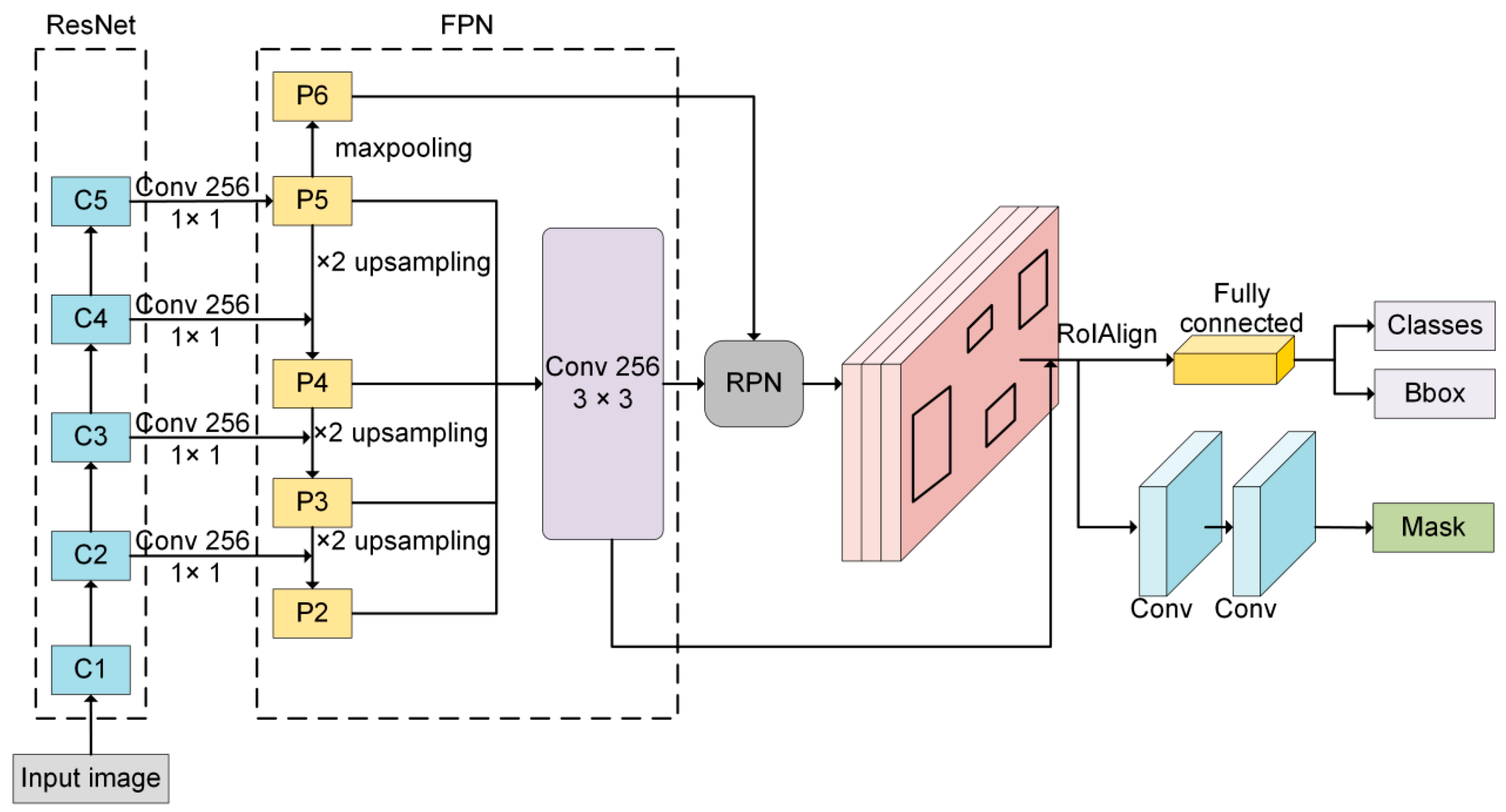
With further developments in deep learning, researchers have developed an advanced instance segmentation model named the Mask region-based convolution neural network (Mask R-CNN), which integrates the core tasks of target detection and semantic segmentation to identify the boundaries of target objects precisely at the pixel level, enabling end-to-end training [29]. Mask R-CNN had made progress in the recognition of targets using high spatial resolution images [30,31]. For example, Wang et al. [30] proposed an automatic extraction algorithm using Mask R-CNN based on multispectral images and achieved crop identification with relatively high accuracy. Zhang et al. [31] proposed an improved Mask R-CNN model for individual tree segmentation and recognition from UAV images with an accuracy of more than 75%. The above methods are based on a single data source and use the idea of sharp changes in the grey scale values of the canopy edges for target object recognition, which has achieved good results in simple and less heterogeneous environments. However, there are more uncertainties in the results in forest environments with high densities, irregular canopy boundaries, and mutual shading [32]. The vertical structure information obtained from LiDAR data is a useful complement to individual tree crown extraction, however, the basic backbone networks of Mask R-CNN (e.g., ResNet50, ResNet101) cannot selectively utilize the unique deep features from each of the multiple data sources [29]. In addition, the cross-entropy loss function ignores the prediction loss of the boundary in the segmentation task, which reduces the accuracy of the segmentation boundary [31]. Therefore, how to fuse the spectral information provided by high spatial resolution image data and the vertical structure information provided by LiDAR data to achieve end-to-end individual tree species classification is an urgent problem needing to be solved [33,34].
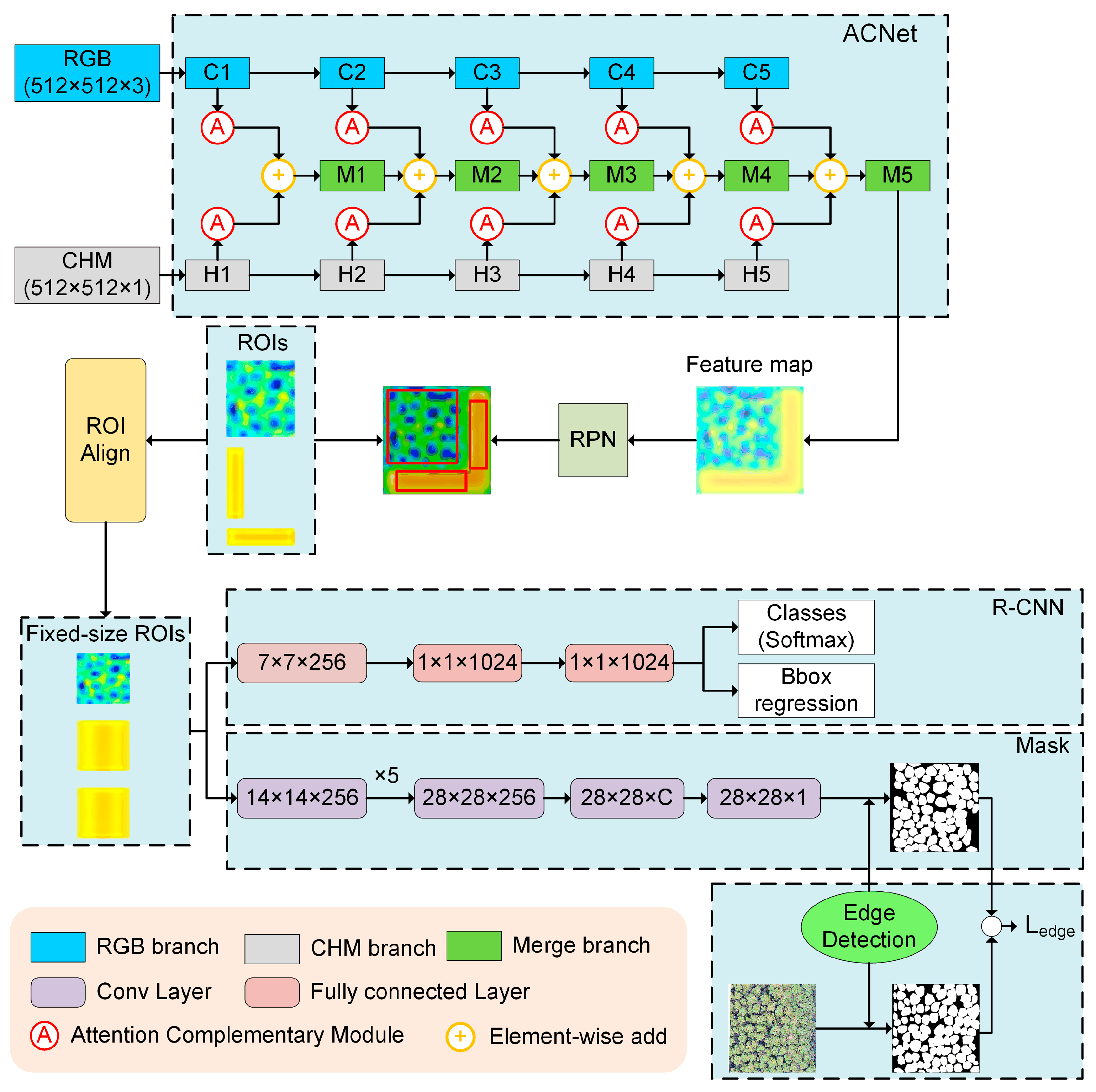
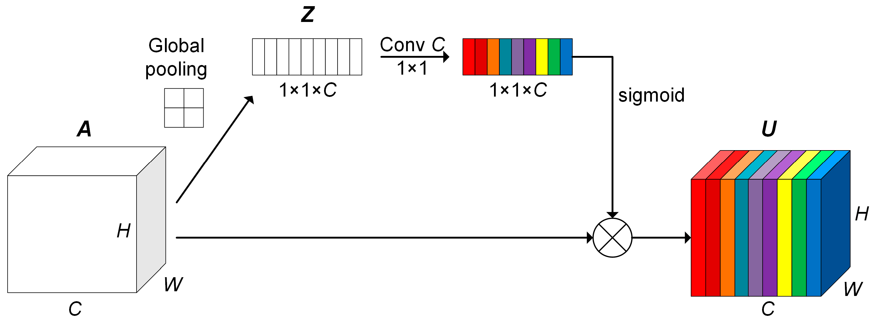
Here, we design an improved Mask R-CNN network named the attention complementary network (ACNet) and edge detection R-CNN (ACE R-CNN) for individual tree species identification in complex forest environments using UAV RGB images and LiDAR data. Firstly, we propose a backbone network named ACNet to replace the basic backbone of Mask R-CNN, which fuses features extracted from high-resolution RGB images and canopy height model (CHM) data by an attention complementary module (ACM). The features extracted from the RGB and CHM branches are weighted and the weighted features are added to the fusion branch by introducing an attention module that can highlight certain important features. We then propose to add an edge loss function, presenting the loss between the predicted and ground-truth mask contours to the Mask R-CNN loss function to improve the edge accuracy of the crown segmentation. The edge loss is computed by introducing an edge detection filter in the Mask branch. Finally, we evaluate the performance of our proposed ACE R-CNN framework for individual tree species identification with different data input methods, different backbone networks, and different edge detection methods in different subregions composed of different tree species. Our proposed ACE R-CNN framework allows for end-to-end individual tree species identification with fast training speed and high accuracy, which provides a new solution for obtaining individual tree-level tree species distribution information in forest resource surveys.

2. Materials and Methods

2.1. Study Area

Gaofeng Forest Farm is a forest plantation in Nanning, Guangxi Province, southern China (22°49′–23°5′N, 108°7′–108°38′E) (Figure 1a), with a cover area of approximately 52 km2. The area has a subtropical monsoon climate with abundant sunshine and rainfall, an average annual temperature of 21.7 °C, and an average annual precipitation of 1300 mm. The topography is mainly hilly, with an elevation of 100~350 m, a slope of 6~35°, and an average slope of approximately 29°. There are thick russet soils and many subtropical and tropical tree species growing here, mainly including Betula alnoides Hamilt. (BH), Michelia macclurei Dandy (MD), Acacia melanoxylon (AM), Eucalyptus urophyllus (EU), Castanopsis hystrix Miq. (CM), Pinus elliottii (PE), and Camellia oleifera Abel (CA). The trees in the plantation are tall with high stand density (Figure 1b,c) and have a complex canopy structure–e.g., various crown sizes, overlapping crowns–which poses a challenge for accurate identification of individual tree species.
Combining subcompartment data from the National Forest Resources of China and Gaofen-2 image data, we selected three experimental areas composed of different tree species to validate our proposed method. These areas had different stand densities and relatively uniform slopes. The first area (Figure 1b) has a size of 180 m × 160 m and the center coordinates are approximately 108°22′6″ E, 22°58′28″ N. This area is dominated by broad-leaved tree species, consisting of Betula alnoides Hamilt., Michelia macclurei Dandy, Acacia melanoxylon, and Other Soft Broads (SB). The second area (Figure 1c) has a size of 180 m × 155 m and the center coordinates are approximately 108°22′6″ E, 22°58′20″ N. It is composed of Acacia melanoxylon, Eucalyptus urophyllus, Castanopsis hystrix Miq., and Other Soft Broads. The third area (Figure 1d) has a size of 105 m × 80 m and the center coordinates are approximately 108°22′5″ E, 22°57′47″ N. This area consists of coniferous and broadleaf trees, with the main tree species consisting of Eucalyptus urophyllus, Pinus elliottii, and Camellia oleifera Abel.

2.2. Remote Sensing Data Collection and Processing

In May 2020, LiDAR data for three experimental areas were obtained using a Riegl VUX-1LR scanner onboard a GV2000 UAV flown at ~250 m above ground level with a strip overlap rate of ~80%. The scanner emits a wavelength of 1550 nm at a scan frequency of 200 Hz. The beam divergence was approximately 0.5 mrad. The point cloud has an average point density of ~45 points/m2. During the same flight, RGB images were acquired using a FC6310R camera (focal length 8.8 mm) at 5472 × 3648 pixels with an exposure time of 1/400 s. The flight direction overlap and the side overlap were about 80%. The LiDAR scanner, camera, and flight parameters are shown in Table 1.
The pre-processing of UAV RGB image data was conducted using LiPPK (Version 1.1, GreenValley International, Beijing, China) and LiMapper (Version 3.1, GreenValley International, Beijing, China), including image position and orientation system (POS) decomposition and orthophoto mosaic. This process generated a RGB orthophotos with a WGS 1984 reference ellipsoid and UTM 49 N projection. The RGB orthophotos has a spatial resolution of 0.08 m.
LiDAR data pre-processing was conducted using LiDAR360 (Version 5.0, GreenValley International, Beijing, China), mainly including resampling, noise point removal, point cloud filtering, and generation of the CHM. Firstly, a Gaussian filtering algorithm [35] was used to remove the noisy points and a modified progressive encrypted triangular mesh filtering algorithm [36] was used to classify the ground points. Then, the digital terrain model (DTM) and digital surface model (DSM) were generated using inverse distance weighted (IDW) algorithm, with a spatial resolution of 0.5 m. The CHM was created by subtracting the DTM from the DSM, which represents the height of real ground objects after removing the terrain background. To reduce the effect of CHM holes, the CHM was processed using the canopy area-controlled CHM null fill method. Finally, the spatial resolution of the CHM was resampled to 0.08 m using the nearest neighbor interpolation method to achieve consistency with the RGB image spatial resolution.
In addition, we used QGIS (Version 3.22, QGIS.ORG) to register the RGB orthophotos and CHM. Ten control points were evenly selected in each area, and the RGB orthophoto and CHM were then corrected using a polynomial correction model, with accuracy controlled within one pixel.

2.3. Individual Tree Species Sample Set Construction

To match the input image requirements of the Mask R-CNN architecture, RGB orthophotos and CHM from three experimental areas were split into 512 × 512-pixel image tiles for processing (Figure 2a,b). Based on a priori knowledge of individual tree species information in the experiment area provided from subcompartment data and ground survey data, we used Lableme (Version 4.6.0, Computer Science and Artificial Intelligence Lab, Massachusetts Institute of Technology, Cambridge, MA, USA) software to construct the individual tree species sample set by manual visual interpretation (Figure 2c). The crown boundary of each tree in the RGB image was manually outlined by the Create Polygon tool and given different labels according to its species information, with different numbers indicating different individual trees under the same species. The individual tree species sample sets were stored in the JSON file format. Then, 60% of the sample set was randomly selected as the training set, and the remaining 40% as the test set. Detailed sample set label information is shown in Table 2. To avoid overfitting during the model training, each image of the training set was rotated (90°, 180°, and 270°) and inverted (horizontally and vertically) at a certain ratio for the data augmentation process.

2.4. Methods

2.4.1. Mask R-CNN Individual Tree Species Identification Framework

Mask R-CNN is a pixel-level multi-target instance segmentation algorithm proposed by He et al. [29]. The network is able to not only accurately classify target instances and output target bounding boxes, but also finely segment the segmentation mask of instances, which achieves the task of simultaneously solving tree species classification, detection, and individual tree crown segmentation [30,37,38,39,40]. The network structure of Mask R-CNN is shown in Figure 3, including the backbone network (Backbone) layer, region proposal network (RPN) layer, region of interest (RoI)-Align layer, and bounding box (Bbox) as well as classification and masks. Specifically, the input to the network is a set/multiset of fixed-size images, and the feature maps are generated by the feature extraction backbone networks of the ResNet and feature pyramid networks (FPN). The RoIs then are extracted using the RPN. The RoIs and the corresponding feature vectors are mapped in the RoIAlign layer with fixed sizes. Finally, the output of the RoIAlign layer is divided into two branches, i.e., the classification detection branch and the Mask prediction branch. The classification detection branch outputs the class with the highest probability and prediction bounding box for each RoI region after a fully-connected layer transformation. The Mask prediction branch uses a convolutional network to generate a binary mask map for the highest confidence class of each RoI region, thus completing the pixel-level segmentation.
The loss function of Mask R-CNN consists of three components: classification error loss (Lcls), bounding box regression error loss (Lbox), and mask segmentation error loss (Lmask). The equations are as follows.
L = L c l s + L b o x + L m a s k ,
where, Mask loss function represents the average binary cross-entropy loss of decoupling the mask branch and the classification branch. For a RoI belonging to the kth class, only the kth mask is considered to be calculated in the loss function. Such a definition allows generating a mask for each category and there is no inter-class competition.

2.4.2. ACE R-CNN: An Improved Mask R-CNN Framework for Individual Tree Species Identification

Since the forest structure in the study area is complex–the canopy boundaries are irregular and blocked by each other–it is difficult to segment the crown and achieve individual tree species identification by only using the idea of mutation of the gray value of the crown boundaries in the RGB images [28,41]. CHM can describe the height variation information of tree crowns and help extract accurate information regarding individual tree crown boundaries [42]. Although the backbone feature extraction network of Mask R-CNN allows the use of CHM as an additional channel to RGB images (in a combined form as input images) [43], the effective information contained in the RGB and CHM images are different and contribute differently to the final target prediction, and the original backbone network treats both data sources equally in the feature extraction process, which easily causes the loss of effective information of CHM. In this study, we integrate the distinct features of high-resolution RGB images and CHM, respectively, and propose a multi-scale feature fusion backbone network named ACNet by introducing an attention complementary module to replace the ResNet-FPN backbone of Mask R-CNN. ACNet can selectively learn features from RGB branches and CHM branches to make the network focus on more important informative regions. In addition, the prediction loss of the boundary in the segmentation task is ignored during the Mask loss calculation in Mask R-CNN, which reduces the accuracy of the segmentation Mask [31,44], and thus we add the edge loss [45] to the mask branch to improve the accuracy of the segmentation result edge. The architecture of our proposed ACE R-CNN network is shown in Figure 4.

ACNet Backbone Network

ACNet is a multi-scale feature fusion network based on the attention mechanism. For the input RGB image and CHM, two complete ResNet branches are deployed to extract features separately. In the forward propagation process, each branch generates a set of feature maps at each module stage, and then extracts weighted features from these feature maps using ACM (Figure 4). The ACM provides a series of attention allocation coefficients (weighting parameters) that can be used to emphasize or select important information about the target processing object and to suppress some irrelevant detailed information. After convolution, the feature maps are further element-wise added to the merge branch, while the others are added to the output of the fusion branch. In this way, low-level and high-level features can be extracted, reorganized, and fused. The specific parameters of the ACNet network structure are shown in Table 3.
Figure 5 shows the ACM in ACNet, assuming that the input feature map A = [A1, ..., Ac] ∈ RC×H×W, where C denotes the number of channels, and H and W denotes the height and width of the feature map, respectively. The output ZRC×1×1 is obtained using global average pooling, the kth position of Z (k ∈ [1, C]) can be expressed as Equation (2).
Z k = 1 H × W i H j W A k ( i , j ) ,
Z is reconstructed by a 1 × 1 convolutional layer with the same number of channels as Z. The 1 × 1 convolutional layer is able to mine the correlation between channels to derive the appropriate weight distribution for these channels. The sigmoid function is then applied to activate the convolution result, constraining the value of the weight vector VRC×1×1 to be between 0 and 1. Finally, we perform the outer product of A and V. The result URC×H×W can be expressed as Equation (3).
U = A σ [ ϕ ( Z ) ] ,
where denotes the outer product, σ denotes the sigmoid function, and ϕ denotes the 1 × 1 convolution. In this way, the feature map A is transformed into a new feature map U, which contains more valid information.

Edge Detection

In order to further improve the accuracy of the segmentation mask, the method of adding edge loss in the mask branch is proposed to make the segmentation boundary more accurate. As shown in the mask branch in Figure 4, the mask corresponding to the correct category is first selected in the 28 × 28 × C output of the mask branch, and then the labeled image is transformed into a binary segmentation map (i.e., the target mask), and finally the prediction mask and the target mask output from the mask branch are taken as input and convolved with the edge detection filter to obtain the edge detection binary output map, and then the edge loss Ledge (Equation (4)).
L e d g e = m e a n ( y y ¯ 2 ) ,
where y denotes the edges detected from the target mask; y ¯ denotes the edges detected from the prediction mask. Thus, the final improved ACE R-CNN loss function is shown in Equation (5).
L = L c l s + L b o x + L m a s k + L e d g e ,
In this study, we used traditional edge detection filters which can be described as a convolution with a 3 × 3 kernel–such as Sobel and Laplacian kernels–to evaluate the effectiveness of the edge loss.
The Sobel operator is a two-dimensional gradient operator to detect edges (Equation (6)). Sx and Sy describes the horizontal and vertical gradient factor of the Sobel operator, respectively. These two factors are convolved with the image I to obtain the horizontal gray value Gx and the vertical gray value Gy (Equation (7)) of each pixel point in the image. The changed gray value (G) is calculated by Equation (8). Here, a threshold value needs to be set for G, where G is greater than this threshold value output is 1, and vice versa output is 0. The final output is the edge detection binary map.
S x = 1 0 1 2 0 2 3 0 1 , S y = 1 2 1 0 0 0 1 2 1 ,
G x = S x I , G y = S y I ,
G = G x 2 + G y 2 ,
The Laplace operator is a second-order differential linear operator (Equation (9)) with the same result in the four 90° directions, i.e., up, down, left, and right. In other words, the operator has no directionality in the 90° direction. In order to make this operator also have this property in the 45° direction, the operator is extended and defined as Equation (10). The edges can be detected by convolution operation with the image.
L = 0 1 0 1 4 1 0 1 0 ,
L = 1 1 1 1 8 1 1 1 1 ,

2.4.3. Experimental Design

To evaluate the performance of Mask R-CNN and ACE R-CNN with different configurations applied to individual tree species identification, we designed five sets of comparative experiments based on different data input types, backbone feature extraction networks, and edge detection filters. The specific experimental design is shown in Table 4.
We used a pre-training ResNet50-FPN architecture framework to initialize the new model in order to speed up the model training and improve the accuracy. The training configuration of the models was specified as follows: batch size was set to 2 and epochs was set to 2000. All models used the same polynomial learning rate (η), with an initial learning rate of 0.001 and an ending learning rate of 0.0001, which decreases at a fixed decreasing rate. Finally, a stochastic gradient descent (SGD) was used as the optimizer with momentum and weight decay set to 0.9 and 0.0001, respectively.
For each experimental area data product, multiple rectangular bounding boxes were predicted around each tree, and each bounding box contained confidence scores for the probability of a tree presence ranging from 0 to 1. In this study, overlapping crowns with confidence scores > 0.3 were retained with the highest confidence scores, and overlapping redundant bounding boxes were removed using a non-maximal suppression algorithm.
In this study, the proposed approach is implemented using the open source PyTorch learning framework and the MMDetection open-source project. The hardware environment is a Dell Precision T7910 (AWT7910) workstation with an IntelR Xeon (R) E5-2620 v4 @2.10 GHZ CPU and an NVIDIA 1080 Ti (12 GB); the operating system is 64-bit Ubuntu 20.02.

2.4.4. Accuracy Evaluation

The intersection-over-union statistic (IoU) was used to evaluate whether the tree-crown polygons were successfully detected (Figure 6). The ground-truth samples as well as the prediction tree bounding boxes were used to calculated IoU. IoU > 0.5 is usually considered as the correct threshold for successful detection [46,47].
P = T P T P + F P ,
R = T P T P + F N ,
F 1 s c o r e = 2 ( P × R ) P + R ,
A P = 0 1 P ( R ) d R ,
where TP is the number of correctly identified trees, FN is the number of trees that were not identified, and FP is the number of extra trees that did not exist in the field.

3. Results

The performance of Mask R-CNN and ACE R-CNN with different input data, backbone networks, and edge detection filters for individual tree species identification were evaluated using test datasets from three experimental areas, and the results are presented in Table 5, Table 6 and Table 7. The distribution maps of individual tree crowns and their species information in the three experimental areas were generated to show the effect of individual tree species identification more clearly (Figure 7). In addition, a confusion matrix was used to show the individual tree species identification results (Figure 8).

3.1. Applicability of Different Input Data on Individual Tree Species Identification

Based on Mask-R-CNN with ResNet50-FPN as the backbone network, we used RGB alone, and RGB and CHM data to identify individual tree species in three experiment areas, namely experiment A and B. The results showed that the combination of RGB with CHM data performed better than RGB data alone (Table 5). With the addition of CHM data, the values of the AP and F1-score were higher, indicating that the accuracy of individual tree species identification was significantly improved. This suggests that CHM data are useful for individual tree species identification.
In Experiment A, the P and R were all lower except for Other Soft Broads in the experiment area 1 (Table 5). The higher P of Other Soft Broads in the experiment area 1 is due to the fact that most individual trees of Other Soft Broads are not detected. As can be seen from the Figure 7 and Figure 8, there were serious missing phenomenon in all three experiment areas when RGB data were used alone. Especially in the experiment area 2, the R of Acacia melanoxylon and Other Soft Broads were all 0. In the experiment B, the phenomenon of missed individual trees detection has been significantly alleviated with RGB and CHM data. It can be concluded that all tree species have better identification results. In the experiment area 1, the P of Betula alnoides Hamilt., Michelia macclurei Dandy, and Acacia melanoxylon achieved 0.8. For Acacia melanoxylon and Eucalyptus urophyllus, the accuracy is significantly improved no matter which experiment area is surveyed, which further demonstrates the importance of CHM data for the identification of individual tree species.

3.2. Effectiveness of Different Backbone Networks for Individual Tree Species Identification

Based on ResNet50-FPN and ACNet backbone networks, the individual tree species identification experiments (Experiment B, C) were carried out in three experiment areas by combining RGB and CHM data. Comparing the data in Table 6, it can be concluded that the ACNet backbone network had superior identification results, with the overall AP of the three areas greater than 0.75. The P, R, F1-score, and AP of all tree species in the three experiment areas obtained by using ACNet were significantly higher than those obtained by ResNet50-FPN backbone networks. With the exception of Michelia macclurei Dandy and Other Soft Broads in the experiment area 1, the APs of individual tree species identification by the ACNet backbone network were all above 0.8. All these indicated that the ACNet backbone network we proposed could significantly improve the accuracy of individual tree species identification.
By analyzing and comparing the results and confusion matrixes (Figure 7 and Figure 8), the phenomenon of missing the detection of individual tree species in the three experiment areas was greatly relieved, and the identification precision was also greatly improved. However, there are still some problems in the identification results. For example, Michelia macclurei Dandy and Other Soft Broads of experiment area 1 have serious missing detection and false identification problems, respectively.
In this study, the three experiment areas selected have different tree species composition with different stand densities, including broad-leaved forests and coniferous and broad-leaved mixed forests, while the same tree species exist in different experiment areas. The results showed that individual tree species identification accuracies of broad-leaved and coniferous tree species were significantly improved under high canopy density conditions using the ACNet. This confirms that the ACNet backbone network has strong universality and robustness in the identification of individual tree species.

3.3. Influence of Edge Detector Filters on Individual Tree Species Identification

In order to better evaluate whether the addition of the edge detection filter will improve the accuracy of individual tree species identification and which kind of edge detection filter is more suitable, three individual tree species identification experiments (experiment C, D, and E) were conducted in the three experiment areas using ACE R-CNN with and without edge detection filter networks, respectively. As shown in the Table 7, the ACE R-CNN that added edge detection filter performed better in individual tree species identification. Among them, the ACE R-CNN with Sobel edge detection filter has the highest accuracy, the AP, P, and F1-score of individual tree species, and the overall AP were all higher than 0.9 in the three experiment areas.
Compared with the ACE R-CNN model without edge detection filter, the R of the ACE R-CNN with Laplacian edge detection filter is improved to a certain extent, but the increase is small. However, the R of ACE R-CNN with Sobel filter is significantly improved, and there is almost no missing detection phenomenon. Especially for Acacia melanoxylon and Eucalyptus urophyllus in Experiment area 1, the problem of ACE R-CNN model in individual tree species identification is effectively solved (Figure 7 and Figure 8).
Moreover, we analyzed the training losses of ACE R-CNN models with/without edge detection filters (Figure 9). The addition of Sobel filter can accelerate the convergence rate of error, and loss is smaller. In other words, the training accuracy of the model with Sobel filter is higher with the same number of epochs. The addition of the Laplace filter has little effect on the convergence speed and accuracy. The effect of individual tree segmentation can be improved by adding edge detection filter in ACE R-CNN because the addition of edge loss could promote the predicted mask edges to gradually match the target mask edges.

4. Discussion

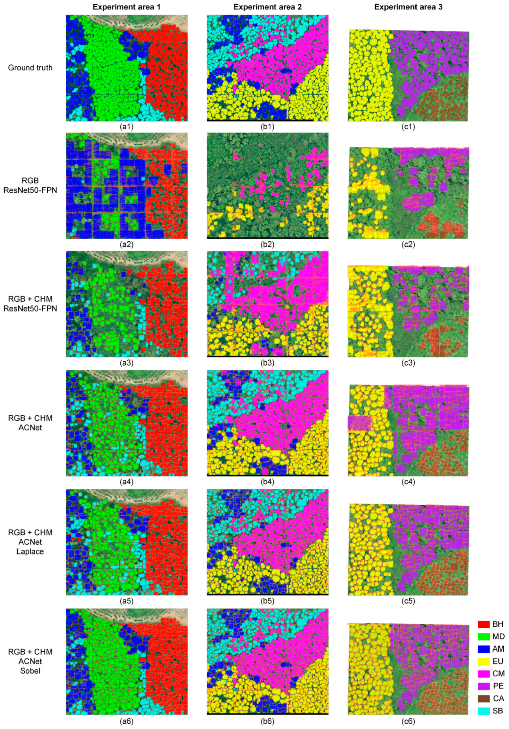
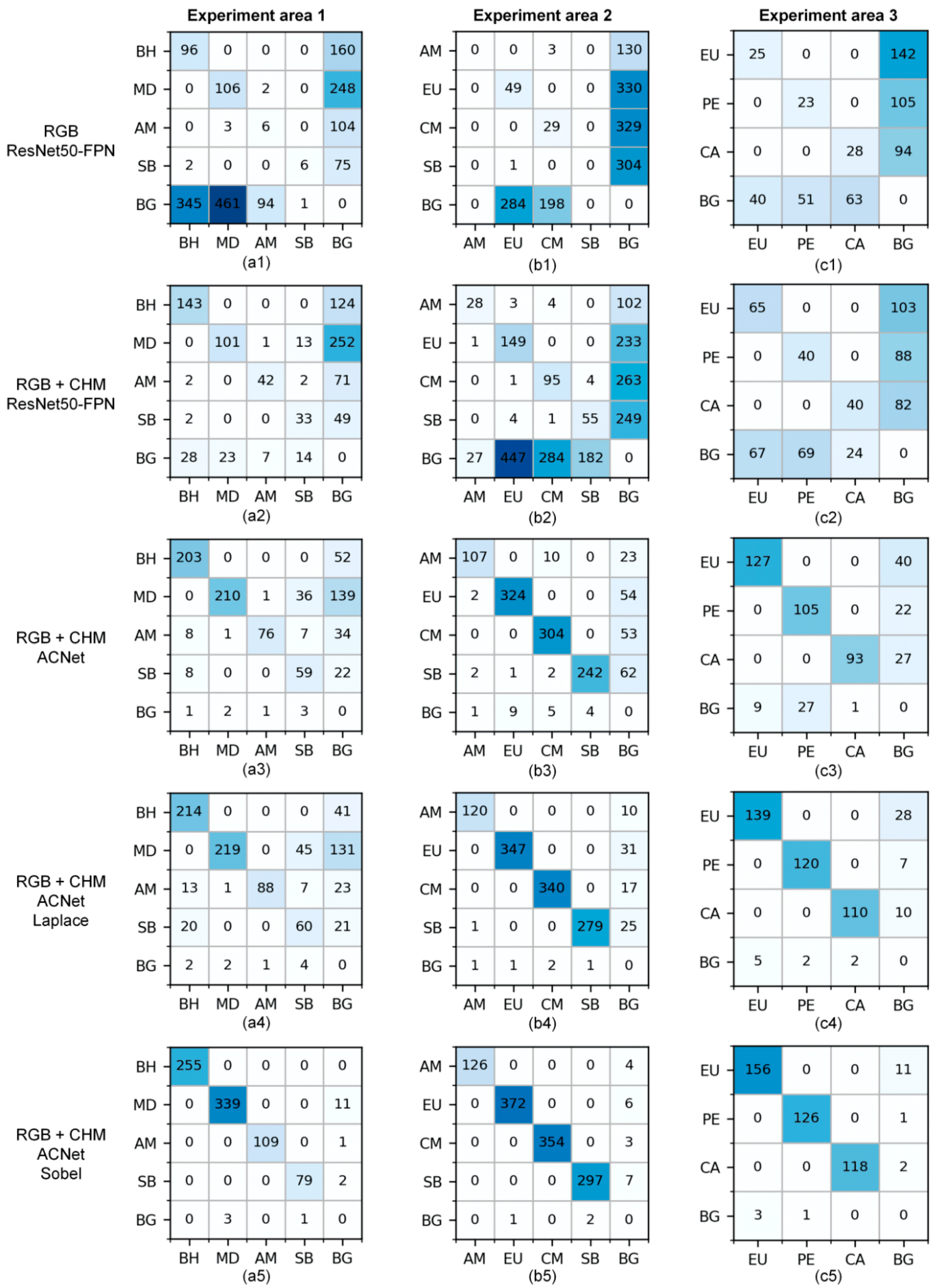
In this study, an instance segmentation framework called ACE R-CNN was designed by introducing the ACM and edge loss to realize identification of individual tree species in an end-to-end manner by integrating UAV high-spatial resolution RGB images and LiDAR data. Compared with traditional Mask R-CNN, which uses only RGB data as data input, the addition of CHM data can significantly improve the accuracy of individual tree species identification (Table 5 and Table 6). This is due to the fact that CHM can provide the height information of vegetation [32], which is important for the identification of individual trees and the determination of crown boundary locations.
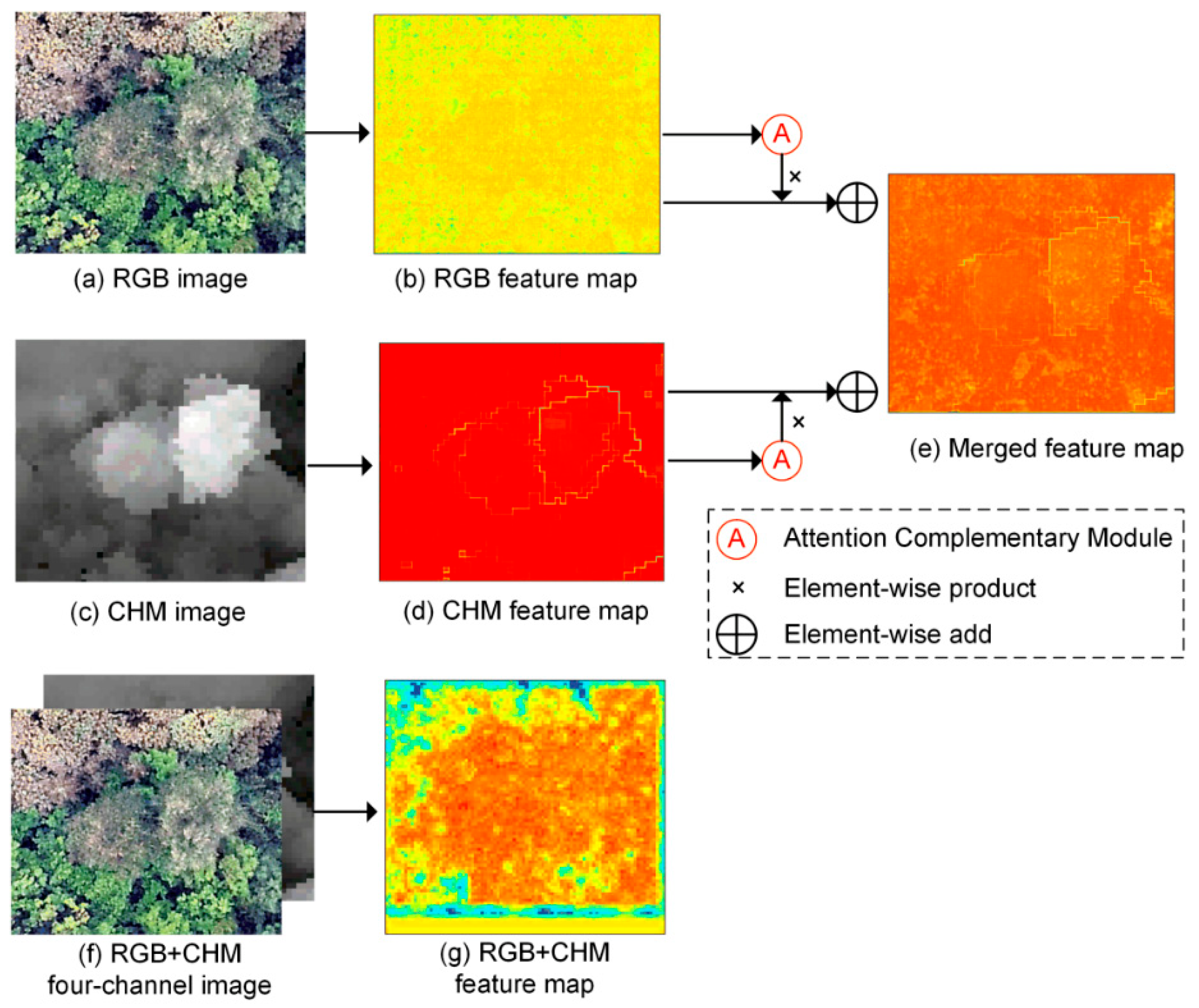
Our proposed ACNet could better facilitate CHM information as a complement to RGB (Table 6). This is because ACNet introduced ACM can selectively learn the combination features of each pixel from RGB and CHM, effectively separating vegetation from the ground surface and helping to complete the identification of individual tree species. We compared the differences in feature extraction backbone networks between ACNet and ResNet50-FPN and visualized some of the results of feature extraction for analysis (Figure 10). In order to match human vision, we choose low-level features from C-2, H-2, M-2 in ACNet, and C-2 in ResNet50-FPN, respectively (Figure 3 and Figure 4). The feature map extracted from the RGB branch (Figure 10b) contains more effective visual information and focuses on the instance content and its global features. The feature map extracted from the CHM branch (Figure 10d) focuses more on the crown boundary information. The feature map of the ACNet fusion branch is shown in Figure 10e. It can be seen that after fusing the features of the two branches, the RGB and CHM information is fully combined, which is beneficial for individual tree information extraction and segmentation. The features (Figure 10g) extracted by ResNet50-FPN from the four-channel image (Figure 10f) composed of RGB and CHM are able to express more crown information than the features extracted using only RGB images (Figure 10b), but the crown boundary information is not prominent, so the performance improvement for segmentation of individual tree instances is limited.
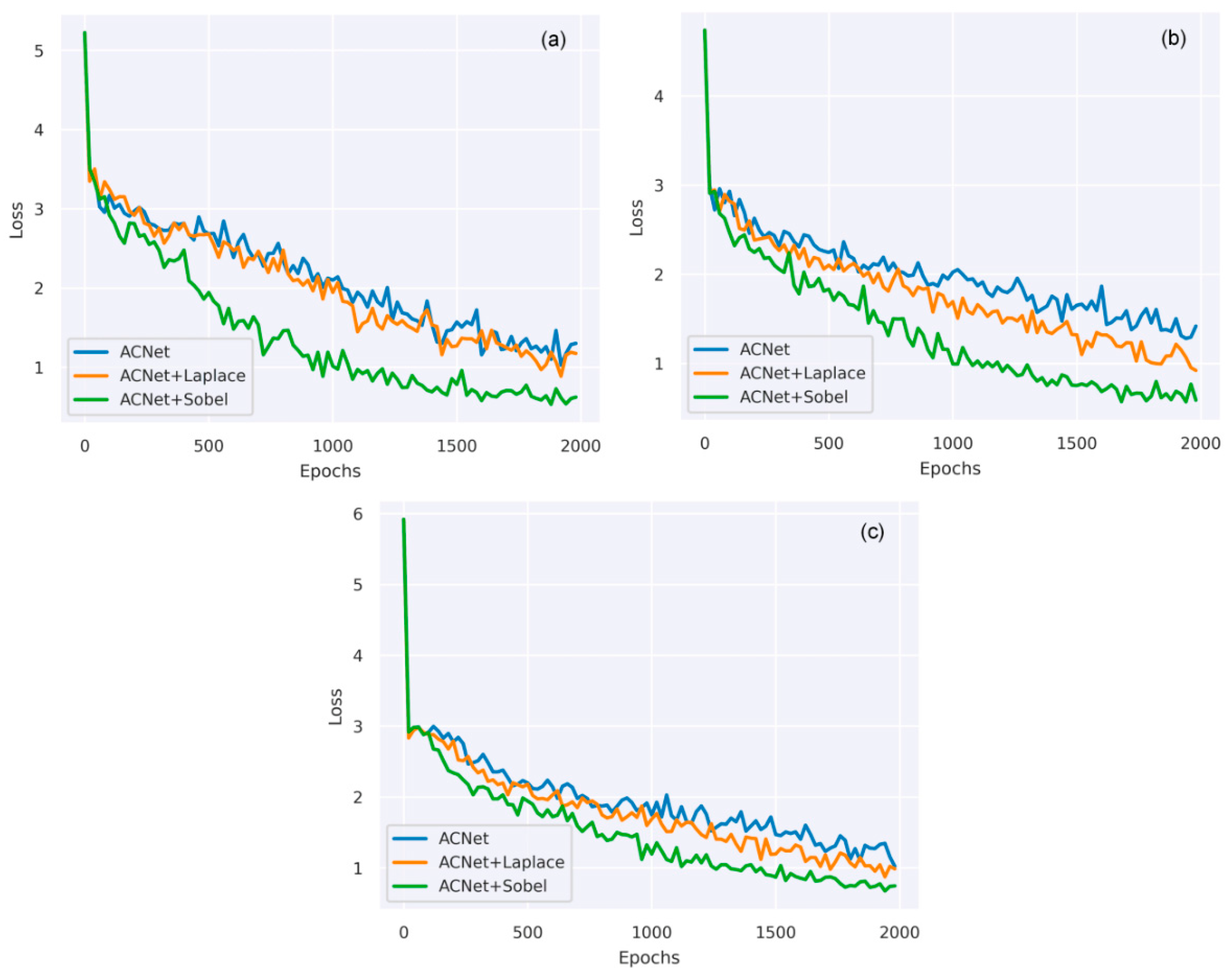
To train the model to have faster speed and improve the training accuracy, we also evaluated the performance of two traditional edge detection filters (Sobel and Laplacian) (Table 7). The performance of ACE R-CNN with edge detection filters for individual tree species identification was significantly improved (Figure 7). This can be attributed to the fact that the addition of edge loss promotes the agreement between the predicted and ground-truth mask edges. The Sobel edge detector is superior to the Laplacian edge detector because the Laplacian edge detector is more susceptible to noise and cannot respond to real edges [48].
It is worth noting that ACE R-CNN uses the spectral information and texture information provided by RGB images for individual tree species identification, and regions with simple tree species composition can achieve better performance (Table 7). However, the spectral information of RGB images includes only three visible bands, and it is difficult to describe the fine spectral features of the tree crown, which will limit the effect of individual tree species identification in forest environments with complex tree species [10]. In future study, high spatial resolution hyperspectral images and LiDAR point cloud data can be used to seek higher accuracy of individual tree species identification [11,49,50,51]. The robustness of the model will be evaluated in areas of more complex natural forests (mixed trees with different species and ages). Furthermore, we will expand the number of samples and balance the proportion of different tree species in dataset [52,53]. Overall, our proposed ACE R-CNN architecture can provide a reference for higher accuracy individual tree species identification in high-density and complex forest environments.

5. Conclusions

In this study, we proposed an improved Mask R-CNN instance segmentation algorithm named ACE R-CNN for individual tree species identification integrating UAV high-spatial resolution RGB images and LiDAR data. ACE R-CNN uses a multi-branch attentional architecture backbone network called ACNet, which is able to selectively complement the weighted features extracted from RGB and CHM branches to the fusion branch by introducing ACM. In addition, edge loss is added into the loss function to further improve the edge precision of the segmentation mask. Through different comparative experiments, the results show that, compared with RGB data alone, the combination of RGB and CHM data is more suitable for individual tree species identification. Compared with the ResNet50-FPN backbone network, the ACNet backbone network has better performance in instance segmentation of individual tree species and could significantly improve the identification accuracy of individual tree species. The ACE R-CNN with an edge detection filter can not only further improve the accuracy of individual tree species identification, but also accelerate the convergence rate of errors. The ACE R-CNN with Sobel filter has the best identification result, with a P, R, F1-score, and AP of tree species all higher than 0.9 in the three test areas. It is a low cost, high-speed, and high efficiency solution for individual tree species identification, and achieves high-precision identification of individual tree species under the high canopy density condition. Moreover, it is of great significance for forest management and forest parameter estimations such as biomass and canopy density.

Author Contributions

Conceptualization, Y.L., G.C. and X.Z.; methodology, Y.L. and G.C.; software, Y.L.; validation, Y.L., G.C., Y.W., L.L. and X.Z.; formal analysis, Y.L.; investigation, X.Z.; resources, X.Z.; data curation, Y.L., G.C., Y.W. and L.L.; writing—original draft preparation, Y.L., G.C., Y.W. and L.L.; writing—review and editing, X.Z.; visualization, Y.L.; supervision, X.Z.; project administration, X.Z.; funding acquisition, X.Z. All authors have read and agreed to the published version of the manuscript.

Funding

This research was funded by the National Natural Science Foundation of China (grant number: 32171779), National Key Research and Development Program of China (grant number: 2017YFD0600900) and DRAGON 5 COOPERATION [ID: 59257].

Acknowledgments

We would like to thank the Gaofeng Forest Farm in Nanning City, Guangxi Province for their aid during the field survey. We also would like to thank Erxue Chen and Lei Zhao from the Institute of Forest Resource Information Techniques, China Academy of Forestry Sciences, and Lin Cao from Nanjing Forestry University for their help in the field work.

Conflicts of Interest

The authors declare that they have no known competing financial interests or personal relationships that could have appeared to influence the work reported in this paper.

References

  1. Hu, B.; Li, Q.; Hall, G.B. A decision-level fusion approach to tree species classification from multi-source remotely sensed data. ISPRS Open J. Photogramm. Remote Sens. 2021, 1, 100002. [Google Scholar] [CrossRef]
  2. Shi, Y.; Skidmore, A.K.; Wang, T.; Holzwarth, S.; Heiden, U.; Pinnel, N.; Zhu, X.; Heurich, M. Tree species classification using plant functional traits from LiDAR and hyperspectral data. Int. J. Appl. Earth Obs. Geoinf. 2018, 73, 207–219. [Google Scholar] [CrossRef]
  3. Torabzadeh, H.; Leiterer, R.; Hueni, A.; Schaepman, M.E.; Morsdorf, F. Tree species classification in a temperate mixed forest using a combination of imaging spectroscopy and airborne laser scanning. Agric. For. Meteorol. 2019, 279, 107744. [Google Scholar] [CrossRef]
  4. Yang, R.; Kan, J. Classification of Tree Species in Different Seasons and Regions Based on Leaf Hyperspectral Images. Remote Sens. 2022, 14, 1524. [Google Scholar] [CrossRef]
  5. Briechle, S.; Krzystek, P.; Vosselman, G. Silvi-Net—A dual-CNN approach for combined classification of tree species and standing dead trees from remote sensing data. Int. J. Appl. Earth Obs. Geoinf. 2021, 98, 102292. [Google Scholar] [CrossRef]
  6. Bruggisser, M.; Roncat, A.; Schaepman, M.E.; Morsdorf, F. Retrieval of higher order statistical moments from full-waveform LiDAR data for tree species classification. Remote Sens. Environ. 2017, 196, 28–41. [Google Scholar] [CrossRef]
  7. Budei, B.C.; St-Onge, B.; Hopkinson, C.; Audet, F.-A. Identifying the genus or species of individual trees using a three-wavelength airborne lidar system. Remote Sens. Environ. 2018, 204, 632–647. [Google Scholar] [CrossRef]
  8. Schiefer, F.; Kattenborn, T.; Frick, A.; Frey, J.; Schall, P.; Koch, B.; Schmidtlein, S. Mapping forest tree species in high resolution UAV-based RGB-imagery by means of convolutional neural networks. ISPRS J. Photogramm. Remote Sens. 2020, 170, 205–215. [Google Scholar] [CrossRef]
  9. Terryn, L.; Calders, K.; Bartholomeus, H.; Bartolo, R.E.; Brede, B.; D’Hont, B.; Disney, M.; Herold, M.; Lau, A.; Shenkin, A.; et al. Quantifying tropical forest structure through terrestrial and UAV laser scanning fusion in Australian rainforests. Remote Sens. Environ. 2022, 271, 112912. [Google Scholar] [CrossRef]
  10. Zhang, B.; Zhao, L.; Zhang, X. Three-dimensional convolutional neural network model for tree species classification using airborne hyperspectral images. Remote Sens. Environ. 2020, 247, 111938. [Google Scholar] [CrossRef]
  11. Mäyrä, J.; Keski-Saari, S.; Kivinen, S.; Tanhuanpää, T.; Hurskainen, P.; Kullberg, P.; Poikolainen, L.; Viinikka, A.; Tuominen, S.; Kumpula, T.; et al. Tree species classification from airborne hyperspectral and LiDAR data using 3D convolutional neural networks. Remote Sens. Environ. 2021, 256, 112322. [Google Scholar] [CrossRef]
  12. Dalponte, M.; Ørka, H.O.; Ene, L.T.; Gobakken, T.; Næsset, E. Tree crown delineation and tree species classification in boreal forests using hyperspectral and ALS data. Remote Sens. Environ. 2014, 140, 306–317. [Google Scholar] [CrossRef]
  13. Lei, L.; Chai, G.; Wang, Y.; Jia, X.; Yin, T.; Zhang, X. Estimating Individual Tree Above-Ground Biomass of Chinese Fir Plantation: Exploring the Combination of Multi-Dimensional Features from UAV Oblique Photos. Remote Sens. 2022, 14, 504. [Google Scholar] [CrossRef]
  14. Liu, L.; Lim, S.; Shen, X.; Yebra, M. A hybrid method for segmenting individual trees from airborne lidar data. Comput. Electron. Agric. 2019, 163, 104871. [Google Scholar] [CrossRef]
  15. Lu, X.; Guo, Q.; Li, W.; Flanagan, J. A bottom-up approach to segment individual deciduous trees using leaf-off lidar point cloud data. ISPRS J. Photogramm. Remote Sens. 2014, 94, 1–12. [Google Scholar] [CrossRef]
  16. Hamraz, H.; Jacobs, N.B.; Contreras, M.A.; Clark, C.H. Deep learning for conifer/deciduous classification of airborne LiDAR 3D point clouds representing individual trees. ISPRS J. Photogramm. Remote Sens. 2019, 158, 219–230. [Google Scholar] [CrossRef] [Green Version]
  17. Goldbergs, G.; Levick, S.R.; Lawes, M.; Edwards, A. Hierarchical integration of individual tree and area-based approaches for savanna biomass uncertainty estimation from airborne LiDAR. Remote Sens. Environ. 2018, 205, 141–150. [Google Scholar] [CrossRef]
  18. Duncanson, L.; Kellner, J.R.; Armston, J.; Dubayah, R.; Minor, D.M.; Hancock, S.; Healey, S.P.; Patterson, P.L.; Saarela, S.; Marselis, S.; et al. Aboveground biomass density models for NASA’s Global Ecosystem Dynamics Investigation (GEDI) lidar mission. Remote Sens. Environ. 2022, 270, 112845. [Google Scholar] [CrossRef]
  19. Jaskierniak, D.; Lucieer, A.; Kuczera, G.; Turner, D.; Lane, P.N.J.; Benyon, R.G.; Haydon, S. Individual tree detection and crown delineation from Unmanned Aircraft System (UAS) LiDAR in structurally complex mixed species eucalypt forests. ISPRS J. Photogramm. Remote Sens. 2021, 171, 171–187. [Google Scholar] [CrossRef]
  20. Dalponte, M.; Bruzzone, L.; Gianelle, D. Tree species classification in the Southern Alps based on the fusion of very high geometrical resolution multispectral/hyperspectral images and LiDAR data. Remote Sens. Environ. 2012, 123, 258–270. [Google Scholar] [CrossRef]
  21. Liu, M.; Han, Z.; Chen, Y.; Liu, Z.; Han, Y. Tree species classification of LiDAR data based on 3D deep learning. Measurement 2021, 177, 109301. [Google Scholar] [CrossRef]
  22. Modzelewska, A.; Fassnacht, F.E.; Stereńczak, K. Tree species identification within an extensive forest area with diverse management regimes using airborne hyperspectral data. Int. J. Appl. Earth Obs. Geoinf. 2020, 84, 101960. [Google Scholar] [CrossRef]
  23. Fassnacht, F.E.; Latifi, H.; Stereńczak, K.; Modzelewska, A.; Lefsky, M.; Waser, L.T.; Straub, C.; Ghosh, A. Review of studies on tree species classification from remotely sensed data. Remote Sens. Environ. 2016, 186, 64–87. [Google Scholar] [CrossRef]
  24. Dalponte, M.; Frizzera, L.; Gianelle, D. Individual tree crown delineation and tree species classification with hyperspectral and LiDAR data. PeerJ 2019, 6, e6227. [Google Scholar] [CrossRef] [PubMed]
  25. Rana, P.; St-Onge, B.; Prieur, J.-F.; Cristina Budei, B.; Tolvanen, A.; Tokola, T. Effect of feature standardization on reducing the requirements of field samples for individual tree species classification using ALS data. ISPRS J. Photogramm. Remote Sens. 2022, 184, 189–202. [Google Scholar] [CrossRef]
  26. Liu, H. Classification of urban tree species using multi-features derived from four-season RedEdge-MX data. Comput. Electron. Agric. 2022, 194, 106794. [Google Scholar] [CrossRef]
  27. Wang, L.; Jia, M.; Yin, D.; Tian, J. A review of remote sensing for mangrove forests: 1956–2018. Remote Sens. Environ. 2019, 231, 111223. [Google Scholar] [CrossRef]
  28. Hu, G.; Yin, C.; Wan, M.; Zhang, Y.; Fang, Y. Recognition of diseased Pinus trees in UAV images using deep learning and AdaBoost classifier. Biosyst. Eng. 2020, 194, 138–151. [Google Scholar] [CrossRef]
  29. He, K.M.; Gkioxari, G.; Dollar, P.; Girshick, R. Mask R-CNN. IEEE Trans. Pattern Anal. Mach. Intell. 2020, 42, 386–397. [Google Scholar] [CrossRef]
  30. Wang, S.; Sun, G.; Zheng, B.; Du, Y. A Crop Image Segmentation and Extraction Algorithm Based on Mask RCNN. Entropy 2021, 23, 1160. [Google Scholar] [CrossRef]
  31. Zhang, C.; Zhou, J.; Wang, H.; Tan, T.; Cui, M.; Huang, Z.; Wang, P.; Zhang, L. Multi-Species Individual Tree Segmentation and Identification Based on Improved Mask R-CNN and UAV Imagery in Mixed Forests. Remote Sens. 2022, 14, 874. [Google Scholar] [CrossRef]
  32. Juntao, Y.; Zhizhong, K.; Sai, C.; Zhou, Y.; Hope, A.P. An individual tree segmentation method based on watershed algorithm and 3D spatial distribution analysis from airborne LiDAR point clouds. IEEE J. Sel. Top. Appl. Earth Obs. Remote Sens. 2020, 13, 1055–1067. [Google Scholar]
  33. Cao, J.; Liu, K.; Zhuo, L.; Liu, L.; Zhu, Y.; Peng, L. Combining UAV-based hyperspectral and LiDAR data for mangrove species classification using the rotation forest algorithm. Int. J. Appl. Earth Obs. Geoinf. 2021, 102, 102414. [Google Scholar] [CrossRef]
  34. Zhao, H.; Zhong, Y.; Wang, X.; Hu, X.; Luo, C.; Boitt, M.; Piiroinen, R.; Zhang, L.; Heiskanen, J.; Pellikka, P. Mapping the distribution of invasive tree species using deep one-class classification in the tropical montane landscape of Kenya. ISPRS J. Photogramm. Remote Sens. 2022, 187, 328–344. [Google Scholar] [CrossRef]
  35. Yang, X.B.; Yang, H.X.; Zhang, F.Q.; Fan, X.J.; Ye, Q.L.; Feng, Z. A random-weighted plane-Gaussian artificial neural network. Neural. Comput. Appl. 2019, 31, 8681–8692. [Google Scholar] [CrossRef]
  36. Duncanson, L.I.; Cook, B.D.; Hurtt, G.C.; Dubayah, R.O. An efficient, multi-layered crown delineation algorithm for mapping individual tree structure across multiple ecosystems. Remote Sens. Environ. 2014, 154, 378–386. [Google Scholar] [CrossRef]
  37. Cao, X.; Pan, J.S.; Wang, Z.; Sun, Z.; Haq, A.U.; Deng, W.; Yang, S. Application of generated mask method based on Mask R-CNN in classification and detection of melanoma—ScienceDirect. Comput. Methods Programs Biomed. 2021, 207, 106174. [Google Scholar] [CrossRef]
  38. Chu, P.; Li, Z.; Lammers, K.; Lu, R.; Liu, X. Deep Learning-based Apple Detection using a Suppression Mask R-CNN. Pattern Recognit. Lett. 2021, 147, 206–211. [Google Scholar] [CrossRef]
  39. Loh, D.R.; Wen, X.Y.; Yapeter, J.; Subburaj, K.; Chandramohanadas, R. A Deep Learning Approach to the Screening of Malaria Infection: Automated and Rapid Cell Counting, Object Detection and Instance Segmentation using Mask R-CNN. Comput. Med. Imaging Graph. 2021, 88, 101845. [Google Scholar] [CrossRef]
  40. Safonova, A.; Guirado, E.; Maglinets, Y.; Alcaraz-Segura, D.; Tabik, S. Olive Tree Biovolume from UAV Multi-Resolution Image Segmentation with Mask R-CNN. Sensors 2021, 21, 1617. [Google Scholar] [CrossRef]
  41. Wu, J.; Yang, G.; Yang, H.; Zhu, Y.; Zhao, C. Extracting apple tree crown information from remote imagery using deep learning. Comput. Electron. Agric. 2020, 174, 105504. [Google Scholar] [CrossRef]
  42. Mongus, D.; Zalik, B. An efficient approach to 3D single tree-crown delineation in LiDAR data. ISPRS J. Photogramm. Remote Sens. 2015, 108, 219–233. [Google Scholar] [CrossRef]
  43. Hao, Z.; Post, C.J.; Mikhailova, E.A.; Lin, L.; Liu, J.; Yu, K. How Does Sample Labeling and Distribution Affect the Accuracy and Efficiency of a Deep Learning Model for Individual Tree-Crown Detection and Delineation. Remote Sens. 2022, 14, 1561. [Google Scholar] [CrossRef]
  44. Zhu, Q.; Du, B.; Yan, P. Boundary-Weighted Domain Adaptive Neural Network for Prostate MR Image Segmentation. IEEE Trans. Med. Imaging 2020, 39, 753–763. [Google Scholar] [CrossRef]
  45. Zimmermann, R.S.; Siems, J.N. Faster training of Mask R-CNN by focusing on instance boundaries. Comput. Vis. Image Underst. 2019, 188, 102795. [Google Scholar] [CrossRef] [Green Version]
  46. Pleoianu, A.I.; Stupariu, M.S.; Sandric, I.; Stupariu, I.; Drǎgu, L. Individual Tree-Crown Detection and Species Classification in Very High-Resolution Remote Sensing Imagery Using a Deep Learning Ensemble Model. Remote Sens. 2020, 12, 2426. [Google Scholar] [CrossRef]
  47. Wu, X.W.; Sahoo, D.; Hoi, S.C.H. Recent advances in deep learning for object detection. Neurocomputing 2020, 396, 39–64. [Google Scholar] [CrossRef] [Green Version]
  48. Luo, J.; Wu, H.; Lei, L.; Wang, H.; Yang, T. GCA-Net: Gait contour automatic segmentation model for video gait recognition. Multimed. Tools Appl. 2021. [Google Scholar] [CrossRef]
  49. Abbas, S.; Peng, Q.; Wong, M.S.; Li, Z.; Wang, J.; Ng, K.T.K.; Kwok, C.Y.T.; Hui, K.K.W. Characterizing and classifying urban tree species using bi-monthly terrestrial hyperspectral images in Hong Kong. ISPRS J. Photogramm. Remote Sens. 2021, 177, 204–216. [Google Scholar] [CrossRef]
  50. Sothe, C.; Dalponte, M.; Almeida, C.M.d.; Schimalski, M.B.; Lima, C.L.; Liesenberg, V.; Miyoshi, G.T.; Tommaselli, A.M.G. Tree Species Classification in a Highly Diverse Subtropical Forest Integrating UAV-Based Photogrammetric Point Cloud and Hyperspectral Data. Remote Sens. 2019, 11, 1338. [Google Scholar] [CrossRef] [Green Version]
  51. Trier, O.D.; Salberg, A.B.; Kermit, M.; Rudjord, O.; Gobakken, T.; Naesset, E.; Aarsten, D. Tree species classification in Norway from airborne hyperspectral and airborne laser scanning data. Eur. J. Remote Sens. 2018, 51, 336–351. [Google Scholar] [CrossRef]
  52. Hartling, S.; Sagan, V.; Sidike, P.; Maimaitijiang, M.; Carron, J. Urban Tree Species Classification Using a WorldView-2/3 and LiDAR Data Fusion Approach and Deep Learning. Sensors 2019, 19, 1284. [Google Scholar] [CrossRef] [Green Version]
  53. Natesan, S.; Armenakis, C.; Vepakomma, U. Individual tree species identification using Dense Convolutional Network (DenseNet) on multitemporal RGB images from UAV. J. Unmanned Veh. Syst. 2020, 8, 310–333. [Google Scholar] [CrossRef]
Figure 1. Overview of the study areas. (a) Location of the study area. (bd) UAV-RGB images, CHM, and photographs of the main tree species for the three experimental areas, respectively.
Remotesensing 14 03035 g001
Figure 2. Schematic diagram of sample labeling for individual tree species identification. (a) RGB orthophotos. (b) 512 × 512-pixel image tile. (c) Tree crown labeling results.
Remotesensing 14 03035 g002
Figure 3. The framework of Mask R-CNN instance segmentation model.
Remotesensing 14 03035 g003
Figure 4. The framework of our proposed ACE R-CNN.
Remotesensing 14 03035 g004
Figure 5. Attention Complementary Module.
Remotesensing 14 03035 g005
Figure 6. Diagram of IoU calculation process. Ctrue is the ground-truth of the crown polygons, Cpredicted is predicted crown polygons.The performance of the Mask R-CNN and ACE R-CNN was evaluated using precision (P), recall (R), F1-score, and average precision (AP). P is the correctness of identified trees, which is the ratio between the number of correctly identified trees and the number of identified trees. R is the individual tree identification rate, which is the ratio between the number of correctly identified trees and the number of ground-truth trees. The F1-score is the overall accuracy of identified trees, which combines P and R. These indicators range from 0 to 1 with larger values indicating higher accuracy, and are calculated based on true positives (TP), false positives (FP), and false negatives (FN) using Equations (11)–(13). Ideally, we would like the model to have higher P and R; however, this relationship is usually negative in reality. With R as the horizontal coordinate and P as the vertical coordinate, the precision–recall curve (PR curve) can be obtained by selecting different confidence thresholds to calculate the values of R and P and plotting the curve. AP is the area under the P–R curve, ranging from 0 to 1 with larger values indicating higher accuracy (Equation (14)).
Remotesensing 14 03035 g006
Figure 7. The results of individual tree species identification for three experimental areas by different experiment schemes. Different experiment schemes are shown on the left of the figure. (ac) Experimental areas 1, 2, and 3, respectively.
Remotesensing 14 03035 g007
Figure 8. The confusion matrix of individual tree species identification for three experimental areas by different experiment schemes. Different experiment schemes are shown on the left of the figure. (ac) Experimental areas 1, 2, and 3, respectively. BG stands for background.
Remotesensing 14 03035 g008
Figure 9. Training loss with different edge detection filters. (ac) Experiment area 1, 2, and 3, respectively.
Remotesensing 14 03035 g009
Figure 10. Feature map extracted by ACNet (ae) and ResNet50-FPN (f,g). (b,d,e) Feature map extracted from the RGB branch, CHM branch, and fusion branch of ACNet, respectively. (g) Feature map extracted by ResNet50-FPN.
Remotesensing 14 03035 g010
Table 1. The LiDAR scanner, camera, and flight parameters.
LiDAR and Flight ParametersRiegl VUX-1LRCamera ParametersFC6310R
Wavelength1550 nmOptical resolution5472 × 3648 pixels
Scanning frequency200 KHzImaging sensor size40.30 × 53.78 mm
Scanning distance5~1350 mImaging focal length8.8 mm
Beam dispersion angle0.5 mradGround Sampling Distance0.08 m
Scan angle±60°Azimuth during imaging
Flight speed7.5 m/s
Flight altitude250 m
Table 2. The number of trees labeled in all image tiles of training set and test set for each species.
Sample SetsTree SpeciesSample Sets
Training SetTest Set
Experiment area 1BH240172
MD291209
AM141106
SB9980
Total771567
Experiment area 2AM146114
EU288212
CM271192
SB235174
Total940692
Experiment area 3EU181135
PE160116
CA147117
Total488368
Table 3. The specific parameters of the ACNet network structure.
Layer NameInput LayerOutput SizeParameters
Input-[2, 512, 512]0
C-1RGB[2, 64, 256, 256]9536
H-1CHM[2, 64, 256, 256]9536
M-1(C-1, H-1)[2, 64, 128, 128]8320
C-2C-1[2, 256, 128, 128]75,008
H-2H-1[2, 256, 128, 128]70,400
M-2(C-2, H-2)[2, 128, 128, 128]666,624
C-3C-2[2, 512, 64, 64]346,368
H-3H-2[2, 512, 64, 64]280,064
M-3(C-3, H-3)[2, 256, 64, 64]3,656,192
C-4C-3[2, 1024, 32, 32]1,380,864
H-4H-3[2, 1024, 32, 32]1,117,184
M-4(C-4, H-4)[2, 2048, 16, 16]26,804,224
C-5C-4[2, 2048, 16, 16]4,462,592
H-5H-4[2, 2048, 16, 16]4,462,592
M-5(C-5, H-5)[2, 256, 16, 16]39,436,800
Total 82,786,304
Note: C: RGB Branch convolution; H: CHM Branch convolution; M: Fusion branch.
Table 4. Comparison experiments with different data input types, backbone networks, and edge detection filters.
ExperimentsModelInput ImageBackboneEdge Detection
AMask R-CNNRGBResNet50-FPNNo
BMask R-CNNRGB + CHMResNet50-FPNNo
CACE R-CNNRGB + CHMACNetNo
DACE R-CNNRGB + CHMACNetLaplacian
EACE R-CNNRGB + CHMACNetSobel
Table 5. Accuracy evaluation of individual tree species identification with different input data.
Experiment SchemeExperiment AreaTree SpeciesPRF1-ScoreAP
AArea 1AM0.0590.0530.0560.029
BArea 1AM0.8400.3590.5030.511
AArea 2AM0.0000.0000.0000.203
BArea 2AM0.5000.2040.2900.442
AArea 1BH0.2170.3750.2750.221
BArea 1BH0.8170.5360.6470.352
AArea 3CA0.3070.2300.2630.085
BArea 3CA0.6250.3280.4300.255
AArea 2CM0.1260.0810.0990.096
BArea 2CM0.2470.2620.2540.296
AArea 2EU0.1470.1290.1370.200
BArea 2EU0.2470.3890.3020.419
AArea 3EU0.3850.1500.2160.119
BArea 3EU0.4920.3870.4330.299
AArea 1MD0.1860.2980.2290.072
BArea 1MD0.8150.2750.4110.454
AArea 3PE0.3110.180.2280.114
BArea 3PE0.3670.3130.3380.264
AArea 1SB0.8570.0720.1330.088
BArea 1SB0.5320.3930.4520.114
AArea 2SB0.0000.0000.0000.121
BArea 2SB0.2280.1780.2000.330
AArea 1Overall0.3300.2000.1730.103
BArea 1Overall0.7510.3910.5030.358
AArea 2Overall0.0680.0530.0590.155
BArea 2Overall0.3060.2580.2620.372
AArea 3Overall0.3340.1870.2360.106
BArea 3Overall0.4950.3430.4000.273
Table 6. Accuracy evaluation of individual tree species identification with different backbone networks.
Experiment SchemeExperiment AreaTree SpeciesPRF1-ScoreAP
BArea 1AM0.840.3590.5030.511
CArea 1AM0.9740.6030.7450.844
BArea 2AM0.5000.2040.2900.442
CArea 2AM0.9550.7640.8490.866
BArea 1BH0.8170.5360.6470.352
CArea 1BH0.9230.7960.8550.859
BArea 3CA0.6250.3280.4300.255
CArea 3CA0.9890.7750.8690.827
BArea 2CM0.2470.2620.2540.296
CArea 2CM0.9470.8520.8970.861
BArea 2EU0.2470.3890.3020.419
CArea 2EU0.9700.8530.9080.885
BArea 3EU0.4920.3870.4330.299
CArea 3EU0.9340.7600.8380.823
BArea 3PE0.3670.3130.3380.264
CArea 3PE0.7950.8270.8110.818
BArea 1SB0.5320.3930.4520.114
CArea 1SB0.5620.6630.6080.678
BArea 2SB0.2280.1780.2000.330
CArea 2SB0.9840.7830.8720.871
BArea 1Overall0.7510.3910.5030.358
CArea 1Overall0.8610.6520.7270.775
BArea 2Overall0.3060.2580.2620.372
CArea 2Overall0.9640.8130.8820.871
BArea 3Overall0.4950.3430.4000.273
CArea 3Overall0.9060.7870.8390.823
Table 7. Accuracy evaluation of individual tree species identification with different edge detection filters.
Experiment SchemeExperiment AreaTree SpeciesPRF1-ScoreAP
CArea 1AM0.9740.6030.7450.844
DArea 1AM0.9890.6670.7960.909
EArea 1AM0.9820.9820.9820.970
CArea 2AM0.9550.7640.8490.866
DArea 2AM0.9830.9230.9520.939
EArea 2AM0.9760.9310.9530.960
CArea 1BH0.9230.7960.8550.859
DArea 1BH0.8590.8390.8490.857
EArea 1BH0.9880.9800.9840.987
CArea 3CA0.9890.7750.8690.827
DArea 3CA0.9820.9170.9480.94
EArea 3CA0.9910.9910.9610.98
CArea 2CM0.9470.8520.8970.861
DArea 2CM0.9940.9520.9730.948
EArea 2CM0.9940.9270.9590.988
CArea 2EU0.970.8530.9080.885
DArea 2EU0.9970.9180.9560.939
EArea 2EU0.9970.9130.9530.989
CArea 3EU0.9340.7600.8380.823
DArea 3EU0.9650.8320.8940.889
EArea 3EU0.9670.8740.9180.949
CArea 1MD0.9860.5440.7010.72
DArea 1MD0.9860.5540.710.81
EArea 1MD0.9790.9260.9520.969
CArea 3PE0.7950.8270.8110.818
DArea 3PE0.9840.9450.9640.926
EArea 3PE0.9760.9690.970.974
CArea 1SB0.5620.6630.6080.678
DArea 1SB0.5170.5940.5530.663
EArea 1SB0.9870.9510.9690.97
CArea 2SB0.9840.7830.8720.871
DArea 2SB0.9960.9150.9540.939
EArea 2SB0.9930.9250.9580.97
CArea 1Overall0.8610.6520.7270.775
DArea 1Overall0.8380.6640.7270.81
EArea 1Overall0.9840.960.9720.974
CArea 2Overall0.9640.8130.8820.871
DArea 2Overall0.9930.9270.9590.941
EArea 2Overall0.990.9240.9560.977
CArea 3Overall0.9060.7870.8390.823
DArea 3Overall0.9770.8980.9350.918
EArea 3Overall0.9780.9450.9500.968
Publisher’s Note: MDPI stays neutral with regard to jurisdictional claims in published maps and institutional affiliations.

