Article

Spatiotemporal Variations of Dryland Vegetation Phenology Revealed by Satellite-Observed Fluorescence and Greenness across the North Australian Tropical Transect

1
Fujian Provincial Key Laboratory of Remote Sensing of Soil Erosion, College of Environment & Safety Engineering, Fuzhou University, Fuzhou 350116, China
2
Faculty of Science, University of Technology Sydney, Ultimo, NSW 2007, Australia
3
College of Science and Engineering, James Cook University, Cairns, QLD 4878, Australia
4
State Key Laboratory of Soil Erosion and Dryland Farming on the Loess Plateau, Northwest A&F University, Xianyang 712100, China
5
Key Lab of Spatial Data Mining & Information Sharing, Ministry of Education of China, Fuzhou 350116, China
*
Author to whom correspondence should be addressed.
Remote Sens. 2022, 14(13), 2985; https://doi.org/10.3390/rs14132985
Submission received: 19 May 2022 / Revised: 17 June 2022 / Accepted: 19 June 2022 / Published: 22 June 2022
(This article belongs to the Special Issue Remote Sensing of Watershed)

Abstract

:
Accurate characterization of spatial patterns and temporal variations in dryland vegetation is of great importance for improving our understanding of terrestrial ecosystem functioning under changing climates. Here, we explored the spatiotemporal variability of dryland vegetation phenology using satellite-observed Solar-Induced chlorophyll Fluorescence (SIF) and the Enhanced Vegetation Index (EVI) along the North Australian Tropical Transect (NATT). Substantial impacts of extreme drought and intense wetness on the phenology and productivity of dryland vegetation are observed by both SIF and EVI, especially in the arid/semiarid interior of Australia without detectable seasonality in the dry year of 2018–2019. The greenness-based vegetation index (EVI) can more accurately capture the seasonal and interannual variation in vegetation production than SIF (EVI r2: 0.47~0.86, SIF r2: 0.47~0.78). However, during the brown-down periods, the rate of decline in EVI is evidently slower than that in SIF and in situ measurement of gross primary productivity (GPP), due partially to the advanced seasonality of absorbed photosynthetically active radiation. Over 70% of the variability of EVI (except for Hummock grasslands) and 40% of the variability of SIF (except for shrublands) can be explained by the water-related drivers (rainfall and soil moisture). By contrast, air temperature contributed to 25~40% of the variability of the effective fluorescence yield (SIFyield) across all biomes. In spite of high retrieval noises and variable accuracy in phenological metrics (MAE: 8~60 days), spaceborne SIF observations, offsetting the drawbacks of greenness-based phenology products with a potentially lagged end of the season, have the promising capability of mapping and characterizing the spatiotemporal dynamics of dryland vegetation phenology.
Keywords:
SIF; EVI; phenology; NATT

Graphical Abstract

1. Introduction

Vegetation phenology, the study of the periodic biological life cycle events of plants, is a critical regulator of carbon and water cycling in terrestrial ecosystems [1]. The trend of global warming has aroused great interest in understanding and monitoring the dynamics of vegetation phenology under the changing climate [2]. As a valuable indicator of climate variability and ecosystem responses [1,3], accurate measurement of land surface phenology (LSP) is crucial for better explicating the land–atmosphere–energy exchange and its representation in terrestrial biosphere models [4,5,6,7].
Phenological studies are usually conducted at the species- or ecosystem-level through ground-based field techniques [4], such as visual inspection, eddy covariance flux towers, near-surface spectral radiometers, and digital cameras [8]. Satellite-based observation, providing a unique and feasible way for examining broader-scale phenomena [4], has notably expanded the horizon of traditional phenology observation [2]. Vegetation indices, which are combinations of surface reflectance at two or more wavelengths designed to highlight a particular property of vegetation [9,10,11], can depict spatiotemporal patterns of the timing of plant growth, senescence, and dormancy at seasonal and inter-annual time scales [12]. The enhanced vegetation index [9], normalized difference vegetation index [13], and leaf area index (LAI) derived from optical satellite sensors are widely applied for tracking large-scale vegetation seasonality.
Dryland vegetation, covering approximately 40% of the global land surface [14], is exceedingly susceptible to climate conditions, mainly owing to chronic physiological stress [10,15,16,17]. Numerous phenology studies based on satellite remote sensing have examined temperature-driven ecosystems of the Northern Hemisphere [4,18,19]; however, the phenological dynamics of dryland vegetation under climate variability and extreme events have not been thoroughly investigated as a result of the intrinsic sensitivity and complexity [15]. Given that the mixed and heterogeneous arrangement of water-limited ecosystems confounds the extraction of the phenophase, Walker et al. (2014) assessed dryland vegetation phenology across an elevation gradient in Arizona, USA, by fusing synthetic Moderate Resolution Imaging Spectroradiometer (MODIS) and Landsat imagery [15]. The significant spatiotemporal variations in savanna biomes with diverse tree-grass ratios implies that grass-containing xeric savanna is especially sensitive and vulnerable to hydro-climatic variability [20]. Besides, previous studies found that growing season retrieved from the greenness-based approach overestimates the photosynthetically active duration, indicating a divergence between greenness and function [21,22]. On the basis of the complex composition of plant functional types, as well as the highly dynamic climate in Australia, accurately assessing the phenological characteristics of dryland vegetation remains challenging [23].
In contrast to the reflectance-based approaches, fluorescence measurements directly from the core of photosynthetic machinery present a fresh manner of remotely sensing vegetation growth and response. Recent studies found that satellite-based observations of SIF can detect interannual and seasonal variations in gross primary production of vegetation in North America [24,25,26]. Wu et al. (2018) found strong spatiotemporal consistency between satellite-based SIF and GPP products across the Contiguous United States [27]. Although photosynthesis and greenness exhibit an analogous seasonality in deciduous forests, satellite chlorophyll fluorescence measurements reveal large-scale decoupling of photosynthesis and greenness dynamics in boreal evergreen forests [28,29]. Continuous observations of satellite-based SIF and vegetation indices contribute to improved understanding of large-scale variations in vegetation phenology and function [21].
By comparing EVI and the photochemical reflectivity index, Smith et al. (2018) demonstrated that chlorophyll fluorescence derived from GOME-2 more accurately captures seasonal and interannual variations of gross primary productivity across dryland ecosystems of southwestern North America [30]. Through evaluating the SIF time series derived from GOME-2 with tower-based GPP in Australia, Sanders et al. (2016) found that natural biome types, such as savanna and open woodland, showed weaker correlations relative to agricultural biomes [31]. Taking into account the sparse spatial resolution of the existing spaceborne SIF product, as well as the varying mixtures of trees, shrubs, and grasses in Australia’s dryland ecosystems, a high-resolution contiguous SIF product (SIFoco2_005) was utilized to explore the phenology dynamics of dryland vegetation along the North Australian Tropical Transect [23]. They found that these up-scaled SIF data at a 0.05° spatial resolution outperformed EVI for characterizing seasonal onset and senescence of dryland vegetation and suggested it had the potential for large-scale mapping of phenology dynamics as opposed to traditional reflectance-based vegetation indices. Nevertheless, SIFoco2_005 was generated by the OCO-2 native SIF along with MODIS reflectance using machine learning [32], and it therefore showed an enhanced accuracy in determining the phenological transition of GPP derived from flux tower measurement as a consequence of it containing both structural and physiological information. However, whether the original SIF observation can accurately capture the phenology dynamics of Australia’s dryland vegetation under climate variability remains unclear.
In arid and semiarid ecosystems, rainfall strongly affects the strength and occurrence of photosynthetic and respiratory activities and is the dominant driver for vegetation phenology and productivity [33,34,35]. The seasonality of Acacia-dominated woodlands (as measured by EVI) was found to show substantial responsiveness to hydroclimatic variability [4]. Additionally, approximately 80% of the variations in the length of the growing season of major dryland biomes along the NATT could be attributed to the variability of annual precipitation [4]. Nevertheless, there is a knowledge gap regarding how and to what extent major environmental and climatic drivers determine the phenological dynamics of fluorescence (as a surrogate of photosynthesis).
The objectives of this study were: (1) to evaluate the spatial patterns and seasonal variations of dryland vegetation phenology across NATT under a dynamic climate; (2) to contrast the differences in phenological metrics derived from satellite-observed SIF and EVI; (3) to determine the dominant factor that drives the interannual and seasonal variability of each vegetation variable among major biome types.

2. Materials and Methods

2.1. Study Area

This study was conducted at a regional scale between 12°S and 23°S and 128°E and 138°E, which is known as the Northern Australian Tropical Transect (Figure 1). This region, particularly the northern NATT, has a classic monsoon climate pattern, which receives more than 80% of its annual precipitation during November to April [4]. From the northern mesic tropics to xeric central Australia, mean annual rainfall ranges from 1700 mm to approximately 300 mm [4].
Correspondingly, the vegetation follows a wet–dry gradient that shifts from Eucalyptus-dominated forests, open forests, and woodlands in the coastal northern areas to Acacia-dominated open woodlands, scattered shrubs, and Hummock grassland into the vast inland [4]. More detailed descriptions with respect to ecosystems, climate, and soils of the entire study region can be found in Ma et al. (2013) and Hutley et al. (2011) [4,36].
To contrast satellite observation with ground-based evidence, we selected five representative flux tower sites across the extensive study area: Howard Springs (AU-How (131.15°E, 12.495°S)), Dry River (AU-Dry (132.371°E, 15.259°S)), Sturt Plains (AU-Stp (133.3502°E, 17.1507°S)), Alice Springs Mulga (AU-ASM, (133.2493°E, 22.2828°S)), and Ti Tree East (AU-TTE (133.64°E, 22.287°S)) [37]. The major vegetation types over the five sites, respectively, are Eucalyptus woodland (AU-How), Eucalyptus open forest (AU-Dry), Tussock grassland (AU-Stp), Mulga open woodland (AU-ASM), and Corymbia savanna (AU-TTE) (http://www.ozflux.org.au/, accessed on 1 October 2020).

2.2. Satellite Data

In this study, we utilised satellite-based SIF records obtained from the Global Ozone Monitoring Experiment-2 (GOME-2) onboard the MetOp-B platform. This dataset is the retrieval of the far-red chlorophyll fluorescence peaking at 740 nm, based on a simplified radiative transfer model in the company of a principal component analysis [22]. Monthly global coverage of SIF data at a 0.5° × 0.5° spatial resolution (level 3, Version 28) from March 2013 to March 2019 was obtained from NASA Goddard Space Flight Centre (https://avdc.gsfc.nasa.gov/, accessed on 1 July 2020). The daily orbital data (level 2, Version) were also used to aggregate 16-day interval records for higher temporal resolution analysis. Given that the data provider of GOME-2 SIF suspended updating in March 2019, we introduced a novel SIF product (from July 2018 to June 2019) derived from TROPOMI onboard the Sentinel-5 Precursor satellite as a supplementary in this study. A data-driven method was employed to retrieve the SIF signal using spectral measurements ranging from 743 nm to 758 nm. The daily orbital TROPOMI SIF at a 0.05° spatial resolution (obtained from ftp://fluo.gps.caltech.edu/data/tropomi/, accessed on 1 August 2020) was likewise aggregated to 16-day series by the mean value.
We used the Moderate Resolution Imaging Spectroradiometer (onboard Aqua, Collection 6) MYD13C1 (0.05°, 16-day) and MYD13C2 (0.05°, monthly) Vegetation Indices’ products from January 2007 to June 2019 downloaded from NASA Earth Observation data (https://search.earthdata.nasa.gov/search, accessed on 1 August 2020). EVI is an optimized version of vegetation indices that effectively reduces soil background influences and is widely used as a proxy of canopy greenness. The equation of EVI is:
E V I = 2.5 ρ N I R ρ r e d ρ N I R + 6 ρ r e d 7.5 ρ b l u e + 1
where ρ b l u e , ρ r e d , and ρ N I R are reflectance in the blue, red, and near-infrared bands, respectively. To reduce noise and uncertainties, only the best-quality data were retained in this study by removing pixels for which the quality control flag of the first 2 bits was neither 00 nor 01, and pixelwise EVI time series data were smoothed using the Savitzky–Golay filter.
MODIS daytime Land Surface Temperature (LST, MYD11C3, Version 6) at a monthly scale and a 0.05° spatial resolution was included in this study, collected from NASA Earth Observation data (https://search.earthdata.nasa.gov/search, accessed on 1 August 2020). Similarly, bad-quality data were removed by eliminating pixels with a quality control flag.
To examine the impact of solar radiation on vegetation seasonality, monthly photosynthetic active radiation (PAR) at a 1° spatial resolution was downloaded from the NASA Langley Research Centre, Cloud and Earth’s Radiant Energy System (CERES, Ed4.1), including adjusted surface PAR, both direct and diffuse fluxes under all-sky conditions (http://ceres.larc.nasa.gov, accessed on 1 August 2020). The total PAR was computed as the sum of both direct and diffuse PAR [38]. As recent studies suggested EVI outperformed the MODIS fPAR (fraction of absorbed PAR) products in estimating the APAR [39], we refer to EVI × PAR as an alternative estimate of APAR:
A P A R   E V I × P A R

2.3. Climate Data and Land Cover Map

To assess the interaction of environmental drivers and vegetation, monthly air temperature (at a 2 m height) and soil moisture content (surface 0–7 cm depth, root zone 28–100 cm depth) based on ERA-5 reanalysis data were downloaded from Copernicus Climate Change Service (https://cds.climate.copernicus.eu/, accessed on 1 July 2020).
Global monthly precipitation based on Integrated Multi-Satellite Retrievals for Global Precipitation Measurement (IMERG, Version 6, Final run, 2007–2019) at a monthly scale and a 0.1° spatial resolution was collected from the NASA Precipitation Processing System (https://pps.gsfc.nasa.gov/, accessed on 1 August 2020).
The National Dynamic Land Cover Dataset (DLCD) was used in this research, obtained from Geoscience Australia and the Bureau of Agricultural and Resource Economics and Sciences (http://www.ga.gov.au/scientific-topics/earth-obs/landcover, accessed on 1 July 2020). Given that some biome types were only covered by a few pixels over the study region, closed Tussock grassland, dense shrubland, and closed forest were, respectively, re-grouped into open/closed Tussock grassland, dense/open shrubland, and closed/open forest (Figure 1). This dataset, validated with abundant field sites, was aggregated to a 0.5° spatial resolution by the most frequent values.

2.4. Eddy Covariance Data

The original level 3 (AU-How, AU-Dry, AU-Stp) and level 6 (AU-ASM, AU-TTE) flux data provided by the OzFlux network (http://www.ozflux.org.au/, accessed on 1 October 2020) were used to pre-process, including quality control assessment, removal of outliers, and gap-filling [33]. In order to estimate daily mean GPP with hourly eddy covariance and meteorological data, flux partitioning for level 3 data was conducted in the open-source R scientific computation environment (Version 3.5.1) associated with the REddyProc package (Version 1.2) [40]. This tool used the gap-filling and flux partitioning algorithms to partition level 3 data into GPP and field ecosystem respiration [41]. The daily-estimated flux data were, respectively, aggregated into monthly and 16-day GPP to match with satellite-based observations.

2.5. Phenological Metrics

Owing to the fact that Ma et al. (2013) demonstrated the capability of singular spectrum analysis (SSA) in the analysis of nonlinear dynamics in NATT [4], we also employed the same method to smooth and reduce the noise in satellite-based SIF, EVI time series. Correspondingly, following Ma et al. (2013) [4], 37 composite periods of the window length and four leading components were selected to configure the parameters in the SSA implementation (Figure 2). After interpolating to daily time series from SSA-reconstructed SIF, EVI series, we used the PhenoDeriv function from the “GreenBrown” package to derive the key phenological metrics. Five metrics were extracted:
  • The start of the growing season (SOS), defined as the date halfway between the minimum value and the fastest greening rate;
  • The peak of the growing season (POS), the date of the maximum value;
  • The end of the growing season (EOS), the date halfway between the fastest brown-down rate and minimum value;
  • The rate of spring green-up (RSP), the amplitude of EVI or SIF between POS and SOS divided by the periods (days) between POS and SOS;
  • The rate of autumn senescence (RAU), the amplitude of EVI or SIF between POS and EOS divided by the periods (days) between POS and EOS
To examine the interaction of environmental drivers and vegetation variables, the coefficient of determination (r2) was calculated across four major biome types. A t-test was utilized to examine the statistical significance level of the relationships (p-value). To further explore the difference between SIF and EVI, we interpreted SIF with fPAR and SIFyield, expressed as:
S I F P A R = S I F P A R
S I F y i e l d = S I F E V I × P A R
Data processing, analysis, and visualization were conducted in the open-source R scientific computation environment (Version 3.6.2) and the associated packages contributed by the R user community (http://cran.r-project.org, accessed on 1 August 2020).

3. Results

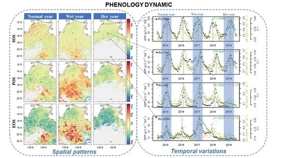
3.1. Seasonal and Inter-Annual Variations over Local Sites

Figure 3 shows the inter-annual variations in eddy-covariance-estimated GPP and satellite-based SIF, EVI over five selected flux sites during 2014–2019. Generally, both satellite variables, especially EVI, exhibited the capacity for capturing the seasonal and inter-annual dynamics of dryland vegetation as indicated by tower-based GPP (r2 ranging from 0.47 to 0.86). Compared with northern mesic sites, the two southern semi-arid sites (AU-ASM, AU-TTE) displayed much higher inter-annual variability, of which there was no seasonality detected by satellite observation nor field measurement in 2018–2019 (Figure 3d,e). Likewise, there was significant hysteretic senescence in EVI as opposed to GPP and SIF over two southern sites, in particular in the wet year of 2016–2017 (Figure 3d,e). The POS of SIF was mostly advanced relative to those of EVI. Furthermore, we found that multi-year series of GOME-2 SIF were more erratic and deviated from the fitted SSA-reconstructed curves than GPP and EVI across northern humid sites, as well as southern arid sites.
To assess the ability of SIF and EVI to track the seasonal dynamics of dryland vegetation as delineated by tower-based GPP, mean seasonal cycles of vegetation variables (normalized to unity at the maxima) over five selected tower sites during 2014–2019 are shown in Figure 4. For northern mesic site AU-How, GOME-2 SIF indicates a consistent growing season with tower data, in contrast to the 1–2-month lagged seasonal profile of EVI during both the green-up and senescent periods (Figure 4a). Conversely, a notably advanced springtime increase and earlier autumn drop are observed in SIF relative to tower-based GPP and EVI for the AU-Dry site (Figure 4b). For three semi-arid and arid sites (AU-Stp, AU-ASM, AU-TTE), both GPP and SIF show a slightly narrower mean seasonal profile as opposed to two northern sites (Figure 4c–e). Besides, there is substantial later senescence in EVI as compared with GPP, SIF, and APAR (≈EVI× PAR) over southern water-limited sites. Likewise, the seasonal profiles of APAR significantly shifted 1~2 months earlier relative to those of EVI over all selected sites.
The differences of key phenological metrics (SOS and EOS) derived from satellite-observed SIF and EVI as compared with tower-based GPP over five flux tower sites during 2014–2019 are presented in Table 1. For SOS over three northern sites (AU-How, AU-Dry, and AU-Stp), the mean absolute errors (MAE) of both SIF and EVI ranging from 7 to 32 days were generally less than those over two southern arid sites (AU-ASM and AU-TTE, ranging from 31 to 54 days). On the contrary, there was a larger discrepancy in EOS at AU-How and AU-Dry (MAE ranges from 39 to 60 days). Besides, for two southern sites (AU-ASM and AU-TTE), the differences of EOS between EVI and GPP were notably larger than those between SIF and GPP.

3.2. Biogeographic Patterns of Vegetation Phenology

To contrast the difference in the timing of seasonal greening derived from two satellite-based vegetation indicators and assess spatial variability over the NATT, the region-wide phenology maps based on EVI (Figure 5) and SIF (Figure 6) were generated. Besides, three representative years, 2014–2015 (normal year), 2016–2017 (wet year), and 2018–2019 (dry year), were selected to evaluate the impact of inter-annual precipitation variability on vegetation phenology. We found large spatial and inter-annual variations in the timing of key phenology transition dates retrieved from EVI (Figure 5), particularly in the southern arid/semi-arid NATT (18°S~23°S). In the extremely dry year of 2018–2019, EVI exhibited no seasonality over nearly the entire southern NATT as compared with detectable phenology in normal and wet years (Figure 5). There is a remarkable lagging trend in key phenological metrics (especially POS and EOS) in 2014–2015 (normal year) and 2016–2017 (wet year) from north to south across the study area, of which Eucalyptus-dominated woodlands distributed in the humid northern NATT started to green-up earlier (September to October). By contrast, the SOS of Acacia-dominated woodlands and Hummock-dominated grasslands distributed in the arid inland was generally 1–2 months behind (November to December). Similarly, the peak and end of the growing season in the south were 2–3 months delayed compared to those in the north during the normal/wet years.
The spatial patterns of vegetation phenology derived from SIF across NATT are shown in Figure 6. Consistent with the in situ comparison, the key phenological metrics of most pixels derived from SIF were generally earlier than those derived from EVI. There was a contrary spatial pattern in the timing of transition dates between EVI and SIF, in which arid/semiarid ecosystems over the southern NATT exhibited advanced POS (December to January) and EOS (March to April) as opposed to POS (February to March) and EOS (April to May) over the northern humid area (Figure 6d–h). With reference to the normal/wet years, larger latitudinal changes in the peak of season between the north (11°S–17°S) and south (17°S–23°S) NATT under the extremely dry condition of 2018–2019 were observed, and fractional pixels in the south were likewise without detectable phenology (Figure 6c,f).
With the purpose of further contrasting the differences in the seasonal profile derived from SIF and EVI, the relationship between green-up rate and brown-down rate of two satellite-based indicators among four major vegetation types are shown in Figure 7. For the semiarid/arid biomes (Hummock grasslands and shrublands), the majority of pixels displayed considerably higher green-up rates than senescence rates (RSPEVI > |RAUEVI|), of which the absolute senescence rate (|RAUEVI|) of Hummock grasslands was mostly less than 0.002 d−1 (Figure 7a,b). By contrast, for northern sub-humid/humid biomes (Eucalyptus-dominated forests and woodlands and Tussock grasslands), there were notably rapid and comparable rates of green-up and senescence (0.0005~0.004 d−1) (Figure 7c,d). On the other hand, RSPSIF and RAUSIF ranging from 0.002~0.010 nW m−2 nm−1 sr−1 d−1 had fewer discrepancies in spite of diverse biomes (Figure 7e–h).

3.3. Interaction between Environmental Drivers and Vegetation Variables

To investigate the dominant factors controlling the seasonal and inter-annual variations in vegetation, the biome-specific relationships of the time series of principle environmental drivers and vegetation variables (SIF, SIFPAR, SIFyield, and EVI) during 2014–2019 are shown in Figure 8. Apart from forests and woodlands, root zone soil moisture was most relevant for EVI (r2: 0.42~0.79) relative to other drivers; among those, temperature-related drivers were poorly correlated (r2 < 0.16) (Figure 8a2–a4). By contrast, both moisture-related drivers, as well as land surface temperature highly corresponded with EVI over northern humid forests and woodlands (Figure 8a1). There were strong correlations (r2 > 0.8) between SIF and EVI over forests and woodlands and Tussock grasslands as compared with moderate correlations (r2: 0.21, 0.38) over water-limited ecosystems (Figure 8b1–b4). Similarly, compared with temperature-related drivers (r2: 0~0.3), water-related factors (especially soil moisture) were more associated with SIF among all biomes. After removing the impact of solar radiation, there was an enhanced agreement between EVI and PAR-normalized SIF (SIFPAR) over Tussock grassland, shrublands, and Hummock grasslands (r2: 0.51~0.86) (Figure 8c2–c4). Likewise, the correlation between root zone soil moisture and SIFPAR was strengthened relative to those with SIF regardless of different vegetation types. Precipitation and surface soil moisture agreed well with the effective fluorescence yield (SIFyield) over forests and woodlands, as well as Tussock grasslands (r2: 0.38~0.62) (Figure 8d1–d2). In addition, there was a moderately increased correlation between air temperature and SIFyield (r2: 0.22~0.4) in comparison to those with SIF or SIFPAR (r2: 0~0.2).

4. Discussion

4.1. Ground Interpretations of the Satellite-Observed Vegetation Phenology

Although the five selected sites exhibited distinct seasonality revealed by eddy covariance flux measurements of vegetation production (GPP), both satellite-based SIF and EVI generally captured seasonal dynamics and inter-annual variations over a variety of biomes (Figure 3 and Figure 4). In comparison with the greenness-based vegetation index, GOME-2 SIF displayed more consistently a seasonal profile with tower-based GPP (Figure 4). Especially, there was a significant “hysteresis effect” during the senescent period of EVI relative to that of GPP over water-limited ecosystems (Hummock grasslands and shrublands), consistent with previous findings [4]. In the wet year of 2016–2017, there was a considerably delayed senescence of EVI over two southern sites (AU-ASM and AU-TTE), relative to those of GPP and SIF (Figure 3). Besides, we found that the autumn senescence rates of EVI were considerably slower than the spring green-up rates of EVI over these arid/semiarid biomes (Figure 7); however, RAU and RSP of SIF were generally comparable. Aside from the slow chlorophyll degradation leading to a gradual decrease of EVI [42], another possible reason causing the discrepancies between EVI and SIF during the brown-down phase is that the rapid decline in solar radiation in the arid southern NATT gave rise to the swiftly dropping SIF signals (Figure 4f). After removing the impact of the PAR on SIF, there was a remarkably enhanced correlation between EVI and SIFPAR across southern water-limited biomes (Figure 8b3–b4).
In contrast to GOME-2 SIF, EVI had an improved capability (higher r2) of tracking the interannual and seasonal variations in GPP over most sites (except AU-Stp, Figure 3), probably owing to the substantial footprint mismatch between flux tower measurement and satellite observations (EVI: ~5 km, SIF: ~50 km). Moreover, as compared with the reflectance-based vegetation index, the high retrieval noises over the low-productivity region resulted in more erratic SIF signals [43], giving rise to a relatively weaker correlation with tower-based GPP. Given the sparse spatial resolution of satellite-based SIF data, Wang et al. (2019) utilized a high-resolution contiguous SIF product (SIFOCO2_005) over the NATT and found that SIFOCO2_005 outperformed EVI at AU-ASM with a stronger temporal consistency with tower-based GPP [23]. However, this up-scaled dataset was generated by native OCO-2 SIF signals along with MODIS reflectance through a machine learning method [32], and it therefore contains information of canopy structure and chlorophyll content, like greenness-based indices. Even though EVI showed a tighter correlation with the GPP (higher r2) than SIFOCO2_005 at AU-Dry and AU-Stp in Wang et al.’s (2019) studies, congruent with our results [23], nevertheless, the high spatiotemporal SIF data derived from TROPOMI onboard the Sentinel-5 Precursor launched in 2017 exhibiting striking consistency with field measurement has great potential of characterizing the phenological dynamics of dryland vegetation in the future [44].

4.2. Spatial Patterns of Vegetation Phenology

Distinct biogeographic patterns in the timing of transition dates, especially POS and EOS, derived from SIF and EVI were observed (Figure 5 and Figure 6), of which there was a considerable latitudinal shift in vegetation phenology (EVI) with a gradually delayed trend from north to south. This is in accordance with the in situ comparison that EVI displayed significantly late senescence at southern xeric sites as compared with GPP and SIF, particularly in the wet year of 2016–2017. In addition, the spatial phenomenon was in line with Ma et al.’s (2013) findings [4], that the majority of EOS based on EVI in wet years (2005–2006, 2010–2011, and 2016–2017), especially in the southern NATT, was generally later than those in normal (2001–2002, 2014–2015) and drought years (2007–2008, 2018–2019) (Figure 5), probably as a consequence of the aforementioned “hysteresis effect”. On the contrary, there was less difference in the spatial patterns of EOS based on SIF between the north and south NATT, as well as in normal/wet years (Figure 6), of which both showed apparently earlier EOS, presumably due to the rapidly decreasing solar radiation over the southern inland. However, as an example of moderately inconsistent phenological metrics compared with field measurement GPP (Table 1), the coarse spatial and temporal resolution of GOME-2 SIF, as well as high retrieval noises, impeded the full potential of capturing the seasonal and interannual variations in vegetation. Considering the drawbacks of existing greenness-based phenology products, as well as the highly heterogeneous composition of dryland ecosystems, our findings imply that new spaceborne SIF with improved spatiotemporal resolution, such as TROPOMI, has great capability for advancing our understanding of phenological characterization in Australia.
Furthermore, SIF and EVI displayed a stronger temporal consistency over northern mesic biomes (forests and woodlands and Tussock grasslands) relative to southern xeric biomes (Hummock grasslands and shrublands) (Figure 8). Soil moisture can explain more than 60% of the seasonal and interannual variability in EVI over most biomes (except Hummock grasslands), suggesting it is the dominant factor controlling the dynamics of vegetation greenness across the NATT. By contrast, the temperature-related drivers could barely explain less than 5% of the variability (except forests and woodlands). Despite the fact that solar radiation has substantial impacts on the SIF signal, temperature- and moisture-related factors almost equally contributed to the process of light use efficiency for fluorescence (SIFyield, except forests and woodlands). This could partially explain the temporal discrepancies between SIF and EVI across diverse biomes.

5. Conclusions

In summary, we utilized satellite-based SIF and EVI observations to investigate the spatial patterns and seasonal dynamics of vegetation phenology across wet and dry years along the North Australian Tropical Transect. Considerable impacts of drought and wet extremes on the phenology and production of dryland vegetation were revealed by both SIF and EVI, especially in the arid/semiarid interior of Australia. Although EVI exhibited a considerably delayed senescence relative to SIF and GPP, phenological metrics derived from SIF had more variable accuracy in contrast to those derived from the greenness-based vegetation index. In addition, EVI exhibiting stronger correlation with tower-based GPP (r2: 0.47~0.86) can be a superior indicator to track the seasonal and interannual variation in dryland vegetation production than the spatially coarse SIF dataset (r2: 0.47~0.78). In spite of the sparse sampling and high retrieval noises of GOME-2 SIF products, which offset the drawbacks of greenness-based phenology products with a potentially lagged end of the season, spaceborne SIF retrieved from state-of-the-art instruments (such as TROPOMI, OCO-2) has the promising potential of assessing the characterization of the phenology dynamics of dryland ecosystems.

Author Contributions

Conceptualization, S.L. and A.H.; methodology, S.L.; validation, S.L.; formal analysis, S.L.; investigation, S.L.; data curation, S.L. and J.C.; writing—original draft preparation, S.L.; writing—review and editing, A.H., Q.Y., R.Z., and Q.W.; visualization, S.L. and Q.W.; supervision, A.H. and Q.Y.; funding acquisition, Q.W. All authors have read and agreed to the published version of the manuscript.

Funding

This research was funded by the Natural Science Foundation of Fujian Province (2021J01627) and the National Natural Science Foundation of China (41601562).

Data Availability Statement

All satellite-based data, as well as other datasets in this study are available from the corresponding author upon reasonable request.

Acknowledgments

The first author acknowledges the financial support from Chinese Scholarship Council, the Ministry of Education, China. We also would like to thank the opening of flux tower data for public access by the Australian Terrestrial Ecosystem Research Network (TERN, Available online: www.tern.org.au)—OzFlux facility (Available online: www.ozflux.org.au, accessed on 1 October 2020).

Conflicts of Interest

The authors declare no conflict of interest.

References

  1. Peng, D.; Wu, C.; Zhang, X.; Yu, L.; Huete, A.R.; Wang, F.; Luo, S.; Liu, X.; Zhang, H. Scaling up Spring Phenology Derived from Remote Sensing Images. Agric. For. Meteorol. 2018, 256–257, 207–219. [Google Scholar] [CrossRef]
  2. Piao, S.; Liu, Q.; Chen, A.; Janssens, I.A.; Fu, Y.; Dai, J.; Liu, L.; Lian, X.; Shen, M.; Zhu, X. Plant Phenology and Global Climate Change: Current Progresses and Challenges. Glob. Change Biol. 2019, 25, 1922–1940. [Google Scholar] [CrossRef] [PubMed]
  3. Zhang, R.; Qi, J.; Leng, S.; Wang, Q. Long-Term Vegetation Phenology Changes and Responses to Preseason Temperature and Precipitation in Northern China. Remote Sens. 2022, 14, 1396. [Google Scholar] [CrossRef]
  4. Ma, X.; Huete, A.; Yu, Q.; Coupe, N.R.; Davies, K.; Broich, M.; Ratana, P.; Beringer, J.; Hutley, L.B.; Cleverly, J. Spatial Patterns and Temporal Dynamics in Savanna Vegetation Phenology across the North Australian Tropical Transect. Remote Sens. Environ. 2013, 139, 97–115. [Google Scholar] [CrossRef]
  5. Zhang, Q.; Kong, D.; Shi, P.; Singh, V.P.; Sun, P. Vegetation Phenology on the Qinghai-Tibetan Plateau and Its Response to Climate Change (1982–2013). Agric. For. Meteorol. 2018, 248, 408–417. [Google Scholar] [CrossRef]
  6. Wang, Q.; Qi, J.; Wu, H.; Zeng, Y.; Shui, W.; Zeng, J.; Zhang, X. Freeze-Thaw Cycle Representation Alters Response of Watershed Hydrology to Future Climate Change. CATENA 2020, 195, 104767. [Google Scholar] [CrossRef]
  7. Wang, Q.; Qi, J.; Qiu, H.; Li, J.; Cole, J.; Waldhoff, S.; Zhang, X. Pronounced Increases in Future Soil Erosion and Sediment Deposition as Influenced by Freeze–Thaw Cycles in the Upper Mississippi River Basin. Environ. Sci. Technol. 2021, 55, 9905–9915. [Google Scholar] [CrossRef]
  8. Verger, A.; Filella, I.; Baret, F.; Peñuelas, J. Vegetation Baseline Phenology from Kilometric Global LAI Satellite Products. Remote Sens. Environ. 2016, 178, 1–14. [Google Scholar] [CrossRef] [Green Version]
  9. Huete, A.; Didan, K.; Miura, T.; Rodriguez, E.P.; Gao, X.; Ferreira, L.G. Overview of the Radiometric and Biophysical Performance of the MODIS Vegetation Indices. Remote Sens. Environ. 2002, 83, 195–213. [Google Scholar] [CrossRef]
  10. Wang, J.; Shi, T.; Yu, D.; Teng, D.; Ge, X.; Zhang, Z.; Yang, X.; Wang, H.; Wu, G. Ensemble Machine-Learning-Based Framework for Estimating Total Nitrogen Concentration in Water Using Drone-Borne Hyperspectral Imagery of Emergent Plants: A Case Study in an Arid Oasis, NW China. Environ. Pollut. 2020, 266, 115412. [Google Scholar] [CrossRef]
  11. Wang, J.; Ding, J.; Li, G.; Liang, J.; Yu, D.; Aishan, T.; Zhang, F.; Yang, J.; Abulimiti, A.; Liu, J. Dynamic Detection of Water Surface Area of Ebinur Lake Using Multi-Source Satellite Data (Landsat and Sentinel-1A) and Its Responses to Changing Environment. CATENA 2019, 177, 189–201. [Google Scholar] [CrossRef]
  12. Broich, M.; Tulbure, M.G.; Verbesselt, J.; Xin, Q.; Wearne, J. Quantifying Australia’s Dryland Vegetation Response to Flooding and Drought at Sub-Continental Scale. Remote Sens. Environ. 2018, 212, 60–78. [Google Scholar] [CrossRef]
  13. Tucker, C.J. Red and Photographic Infrared Linear Combinations for Monitoring Vegetation. Remote Sens. Environ. 1979, 8, 127–150. [Google Scholar] [CrossRef] [Green Version]
  14. Reynolds, J.F.; Smith, D.M.S.; Lambin, E.F.; Turner, B.L.; Mortimore, M.; Batterbury, S.P.J.; Downing, T.E.; Dowlatabadi, H.; Fernández, R.J.; Herrick, J.E. Global Desertification: Building a Science for Dryland Development. Science 2007, 316, 847–851. [Google Scholar] [CrossRef] [Green Version]
  15. Walker, J.J.; de Beurs, K.M.; Wynne, R.H. Dryland Vegetation Phenology across an Elevation Gradient in Arizona, USA, Investigated with Fused MODIS and Landsat Data. Remote Sens. Environ. 2014, 144, 85–97. [Google Scholar] [CrossRef]
  16. Zeng, J.; Zhang, R.; Qu, Y.; Bento, V.A.; Zhou, T.; Lin, Y.; Wu, X.; Qi, J.; Shui, W.; Wang, Q. Improving the Drought Monitoring Capability of VHI at the Global Scale via Ensemble Indices for Various Vegetation Types from 2001 to 2018. Weather. Clim. Extrem. 2022, 35, 100412. [Google Scholar] [CrossRef]
  17. Zhang, J.; Ding, J.; Wu, P.; Tan, J.; Huang, S.; Teng, D.; Cao, X.; Wang, J.; Chen, W. Assessing Arid Inland Lake Watershed Area and Vegetation Response to Multiple Temporal Scales of Drought Across the Ebinur Lake Watershed. Sci. Rep. 2020, 10, 1354. [Google Scholar] [CrossRef]
  18. Wang, J.; Ding, J.; Yu, D.; Ma, X.; Zhang, Z.; Ge, X.; Teng, D.; Li, X.; Liang, J.; Lizaga, I.; et al. Capability of Sentinel-2 MSI Data for Monitoring and Mapping of Soil Salinity in Dry and Wet Seasons in the Ebinur Lake Region, Xinjiang, China. Geoderma 2019, 353, 172–187. [Google Scholar] [CrossRef]
  19. Wang, J.; Hu, X.; Shi, T.; He, L.; Hu, W.; Wu, G. Assessing Toxic Metal Chromium in the Soil in Coal Mining Areas via Proximal Sensing: Prerequisites for Land Rehabilitation and Sustainable Development. Geoderma 2022, 405, 115399. [Google Scholar] [CrossRef]
  20. Ma, X.; Huete, A.; Moore, C.E.; Cleverly, J.; Hutley, L.B.; Beringer, J.; Leng, S.; Xie, Z.; Yu, Q.; Eamus, D. Spatiotemporal Partitioning of Savanna Plant Functional Type Productivity along NATT. Remote Sens. Environ. 2020, 246, 111855. [Google Scholar] [CrossRef]
  21. Jeong, S.-J.; Schimel, D.; Frankenberg, C.; Drewry, D.T.; Fisher, J.B.; Verma, M.; Berry, J.A.; Lee, J.-E.; Joiner, J. Application of Satellite Solar-Induced Chlorophyll Fluorescence to Understanding Large-Scale Variations in Vegetation Phenology and Function over Northern High Latitude Forests. Remote Sens. Environ. 2017, 190, 178–187. [Google Scholar] [CrossRef]
  22. Joiner, J.; Yoshida, Y.; Vasilkov, A.P.; Schaefer, K.; Jung, M.; Guanter, L.; Zhang, Y.; Garrity, S.; Middleton, E.M.; Huemmrich, K.F.; et al. The Seasonal Cycle of Satellite Chlorophyll Fluorescence Observations and Its Relationship to Vegetation Phenology and Ecosystem Atmosphere Carbon Exchange. Remote Sens. Environ. 2014, 152, 375–391. [Google Scholar] [CrossRef] [Green Version]
  23. Wang, C.; Beringer, J.; Hutley, L.B.; Cleverly, J.; Li, J.; Liu, Q.; Sun, Y. Phenology Dynamics of Dryland Ecosystems along the North Australian Tropical Transect Revealed by Satellite Solar-induced Chlorophyll Fluorescence. Geophys. Res. Lett. 2019, 46, 5294–5302. [Google Scholar] [CrossRef]
  24. Yang, X.; Tang, J.; Mustard, J.F.; Lee, J.-E.; Rossini, M.; Joiner, J.; Munger, J.W.; Kornfeld, A.; Richardson, A.D. Solar-Induced Chlorophyll Fluorescence That Correlates with Canopy Photosynthesis on Diurnal and Seasonal Scales in a Temperate Deciduous Forest. Geophys. Res. Lett. 2015, 42, 2977–2987. [Google Scholar] [CrossRef]
  25. Zhang, Y.; Xiao, X.; Jin, C.; Dong, J.; Zhou, S.; Wagle, P.; Joiner, J.; Guanter, L.; Zhang, Y.; Zhang, G.; et al. Consistency between Sun-Induced Chlorophyll Fluorescence and Gross Primary Production of Vegetation in North America. Remote Sens. Environ. 2016, 183, 154–169. [Google Scholar] [CrossRef] [Green Version]
  26. Zuromski, L.M.; Bowling, D.R.; Köhler, P.; Frankenberg, C.; Goulden, M.L.; Blanken, P.D.; Lin, J.C. Solar-Induced Fluorescence Detects Interannual Variation in Gross Primary Production of Coniferous Forests in the Western United States. Geophys. Res. Lett. 2018, 45, 7184–7193. [Google Scholar] [CrossRef]
  27. Wu, X.; Xiao, X.; Zhang, Y.; He, W.; Wolf, S.; Chen, J.; He, M.; Gough, C.M.; Qin, Y.; Zhou, Y. Spatiotemporal Consistency of Four Gross Primary Production Products and Solar-Induced Chlorophyll Fluorescence in Response to Climate Extremes Across CONUS in 2012. J. Geophys. Res. Biogeosci. 2018, 123, 3140–3161. [Google Scholar] [CrossRef]
  28. Chang, Q.; Xiao, X.; Jiao, W.; Wu, X.; Doughty, R.; Wang, J.; Du, L.; Zou, Z.; Qin, Y. Assessing Consistency of Spring Phenology of Snow-Covered Forests as Estimated by Vegetation Indices, Gross Primary Production, and Solar-Induced Chlorophyll Fluorescence. Agric. For. Meteorol. 2019, 275, 305–316. [Google Scholar] [CrossRef]
  29. Walther, S.; Voigt, M.; Thum, T.; Gonsamo, A.; Zhang, Y.; Kohler, P.; Jung, M.; Varlagin, A.; Guanter, L. Satellite Chlorophyll Fluorescence Measurements Reveal Large-Scale Decoupling of Photosynthesis and Greenness Dynamics in Boreal Evergreen Forests. Glob. Chang. Biol. 2016, 22, 2979–2996. [Google Scholar] [CrossRef] [Green Version]
  30. Smith, W.K.; Biederman, J.A.; Scott, R.L.; Moore, D.J.P.; He, M.; Kimball, J.S.; Yan, D.; Hudson, A.; Barnes, M.L.; MacBean, N.; et al. Chlorophyll Fluorescence Better Captures Seasonal and Interannual Gross Primary Productivity Dynamics Across Dryland Ecosystems of Southwestern North America. Geophys. Res. Lett. 2018, 45, 748–757. [Google Scholar] [CrossRef]
  31. Sanders, A.; Verstraeten, W.; Kooreman, M.; van Leth, T.; Beringer, J.; Joiner, J. Spaceborne Sun-Induced Vegetation Fluorescence Time Series from 2007 to 2015 Evaluated with Australian Flux Tower Measurements. Remote Sens. 2016, 8, 895. [Google Scholar] [CrossRef] [Green Version]
  32. Yu, L.; Wen, J.; Chang, C.Y.; Frankenberg, C.; Sun, Y. High-Resolution Global Contiguous SIF of OCO-2. Geophys. Res. Lett. 2019, 46, 1449–1458. [Google Scholar] [CrossRef]
  33. Cleverly, J.; Chen, C.; Boulain, N.; Villalobos-Vega, R.; Faux, R.; Grant, N.; Yu, Q.; Eamus, D. Aerodynamic Resistance and Penman–Monteith Evapotranspiration over a Seasonally Two-Layered Canopy in Semiarid Central Australia. J. Hydrometeorol. 2013, 14, 1562–1570. [Google Scholar] [CrossRef] [Green Version]
  34. Wang, Q.; Zhang, R.; Qi, J.; Zeng, J.; Wu, J.; Shui, W.; Wu, X.; Li, J. An Improved Daily Standardized Precipitation Index Dataset for Mainland China from 1961 to 2018. Scientific Data 2022, 9, 124. [Google Scholar] [CrossRef] [PubMed]
  35. Wang, Q.; Zeng, J.; Leng, S.; Fan, B.; Tang, J.; Jiang, C.; Huang, Y.; Zhang, Q.; Qu, Y.; Wang, W.; et al. The Effects of Air Temperature and Precipitation on the Net Primary Productivity in China during the Early 21st Century. Front. Earth Sci. 2018, 12, 818–833. [Google Scholar] [CrossRef]
  36. Hutley, L.B.; Beringer, J.; Isaac, P.R.; Hacker, J.M.; Cernusak, L.A. A Sub-Continental Scale Living Laboratory: Spatial Patterns of Savanna Vegetation over a Rainfall Gradient in Northern Australia. Agric. For. Meteorol. 2011, 151, 1417–1428. [Google Scholar] [CrossRef]
  37. Beringer, J.; Hutley, L.B.; McHugh, I.; Arndt, S.K.; Campbell, D.; Cleugh, H.A.; Cleverly, J.; de Dios, V.R.; Eamus, D.; Evans, B. An Introduction to the Australian and New Zealand Flux Tower Network-OzFlux. Biogeosciences 2016, 13, 5895–5916. [Google Scholar] [CrossRef] [Green Version]
  38. Wang, X.; Qiu, B.; Li, W.; Zhang, Q. Impacts of Drought and Heatwave on the Terrestrial Ecosystem in China as Revealed by Satellite Solar-Induced Chlorophyll Fluorescence. Sci. Total Environ. 2019, 693, 133627. [Google Scholar] [CrossRef]
  39. Lu, X.; Cheng, X.; Li, X.; Chen, J.; Sun, M.; Ji, M.; He, H.; Wang, S.; Li, S.; Tang, J. Seasonal Patterns of Canopy Photosynthesis Captured by Remotely Sensed Sun-Induced Fluorescence and Vegetation Indexes in Mid-to-High Latitude Forests: A Cross-Platform Comparison. Sci. Total Environ. 2018, 644, 439–451. [Google Scholar] [CrossRef]
  40. Wutzler, T.; Lucas-Moffat, A.; Migliavacca, M.; Knauer, J.; Sickel, K.; Šigut, L.; Menzer, O.; Reichstein, M. Basic and Extensible Post-Processing of Eddy Covariance Flux Data with REddyProc. Biogeosciences 2018, 15, 5015–5030. [Google Scholar] [CrossRef] [Green Version]
  41. Reichstein, M.; Falge, E.; Baldocchi, D.; Papale, D.; Aubinet, M.; Berbigier, P.; Bernhofer, C.; Buchmann, N.; Gilmanov, T.; Granier, A. On the Separation of Net Ecosystem Exchange into Assimilation and Ecosystem Respiration: Review and Improved Algorithm. Glob. Chang. Biol. 2005, 11, 1424–1439. [Google Scholar] [CrossRef]
  42. Jenkins, J.P.; Richardson, A.D.; Braswell, B.H.; Ollinger, S.v.; Hollinger, D.Y.; Smith, M.-L. Refining Light-Use Efficiency Calculations for a Deciduous Forest Canopy Using Simultaneous Tower-Based Carbon Flux and Radiometric Measurements. Agric. For. Meteorol. 2007, 143, 64–79. [Google Scholar] [CrossRef]
  43. Geruo, A.; Velicogna, I.; Kimball, J.S.; Du, J.; Kim, Y.; Colliander, A.; Njoku, E. Satellite-Observed Changes in Vegetation Sensitivities to Surface Soil Moisture and Total Water Storage Variations since the 2011 Texas Drought. Environ. Res. Lett. 2017, 12, 054006. [Google Scholar]
  44. Leng, S.; Huete, A.; Cleverly, J.; Gao, S.; Yu, Q.; Meng, X.; Qi, J.; Zhang, R.; Wang, Q. Assessing the Impact of Extreme Droughts on Dryland Vegetation by Multi-Satellite Solar-Induced Chlorophyll Fluorescence. Remote Sens. 2022, 14, 1581. [Google Scholar] [CrossRef]
Figure 1. (a) Land cover map of the Northern Australian Tropical Transect (NATT) study area (data source: Dynamic Land Cover Dataset). Black triangles refer to the five flux tower sites. Photographs show the ground-view of each flux tower site linked with the black arrow (image source: www.ozflux.org.au, accessed on 1 October 2020). (b) The locations of the study area over the Australian continent (image source: Google Earth).
Remotesensing 14 02985 g001
Figure 2. Schematic diagram of phenological metrics’ retrieval. The curve refers to the seasonal SSA-re-reconstructed EVI or SIF profile at a daily scale. SOS: the start of the growing season; POS: the peak of the growing season; EOS: the end of the growing season; RSP: the rate of spring green-up; RAU: the rate of autumn senescence.
Remotesensing 14 02985 g002
Figure 3. Time series of SSA-reconstructed tower-based GPP, GOME-2 SIF, MODIS EVI over (a) AU-How, (b) AU-Dry, (c) AU-Stp, (d) AU-ASM, and (e) AU-TTE. R-squared (r2) refers to the relationship between GPP and EVI (green) and GPP and SIF (orange), respectively. Vertical dashed lines refer to the peak of the growing season in each hydrological year.
Remotesensing 14 02985 g003
Figure 4. (ae) Seasonal cycle (mean) of tower-based GPP, GOME-2 SIF, MODIS EVI, and EVI × PAR over 5 selected local sites during 2014–2019. Curves are normalized with respect to unity at the maximum annual value. (f) Seasonal cycle (mean) of PAR over 5 selected local sites during 2014–2019. Satellite observations were extracted within a 3 × 3 window centred at each flux tower site (SIF: 1.5° × 1.5°; EVI and EVI × PAR: 0.15° × 0.15°).
Remotesensing 14 02985 g004
Figure 5. Spatial patterns of vegetation phenology based on EVI over the NATT study area across three representative hydrological years, (a,d,g) 2014–2015 (normal year), (b,e,h) 2016–2017 (wet year), and (c,f,i) 2018–2019 (dry year). The filled pixels (grey shaded areas) are either water body or without detectable phenology. SOS: the start of growing season; POS: the peak of growing season; EOS: the end of growing season. Blank circles represent 5 selected eddy covariance flux tower sites.
Remotesensing 14 02985 g005
Figure 6. Spatial patterns of vegetation phenology based on (ah) GOME-2 SIF and (ik) TROPOMI SIF over the NATT study area across three representative hydrological years, 2014–2015 (normal year), 2016–2017 (wet year), and 2018–2019 (dry year). The filled pixels (grey shaded areas) are either water body or without detectable phenology. SOS: the start of growing season; POS: the peak of growing season; EOS: the end of growing season. Blank circles represent 5 selected eddy covariance flux tower sites.
Remotesensing 14 02985 g006
Figure 7. Scatter plot between spring green-up rates (RSP) and autumn senescence rates (RAU) of (ad) EVI and (eh) SIF among four major biomes across the entire study region. Red dashed lines refer to a −1:1 diagonal.
Remotesensing 14 02985 g007
Figure 8. Relationships between climatic–environmental drivers and vegetation variables of (a1a4) EVI, (b1b4) SIF, (c1c4) SIFPAR, and (d1d4) SIFyield among four major biome types across the NATT during 2014–2019. (p-value < 0.001).
Remotesensing 14 02985 g008
Table 1. Summary of differences (days) in SOS and EOS derived from SIF, EVI compared with that derived from tower-based GPP. Negative values represent an earlier green-up (SOS) or senescence (EOS) of SIF, EVI relative to that of GPP.
SOSEOS
SiteData2014–20152015–20162016–20172017–20182018–2019MAE 12014–20152015–20162016–20172017–20182018–2019MAE
AU-HowSIF-GPP624−4−21011−8020744−4239
EVI-GPP−17−12103−61097483241541
AU-DrySIF-GPP−563−53−38−1032−63−71−42−47−7560
EVI-GPP−65−27−16−812−39−55−5−23−78 40
AU-StpSIF-GPP2−21−33−21 19−5−14−140 8
EVI-GPP−30617 73122210 12
AU-ASMSIF-GPP22108−25 52−119−31 17
EVI-GPP3786−10 44148434 44
AU-TTESIF-GPP15−134−13 54−29−27 13
EVI-GPP67−251 31208442 49
1 MAE: mean absolute error.
Publisher’s Note: MDPI stays neutral with regard to jurisdictional claims in published maps and institutional affiliations.

