
Turbulence Detection in the Atmospheric Boundary Layer Using Coherent Doppler Wind Lidar and Microwave Radiometer


Abstract
:
1. Introduction
2. Principle
2.1. Stable Stratification
2.2. Convective Boundary Layer
3. Experiments
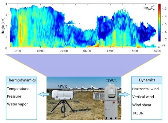
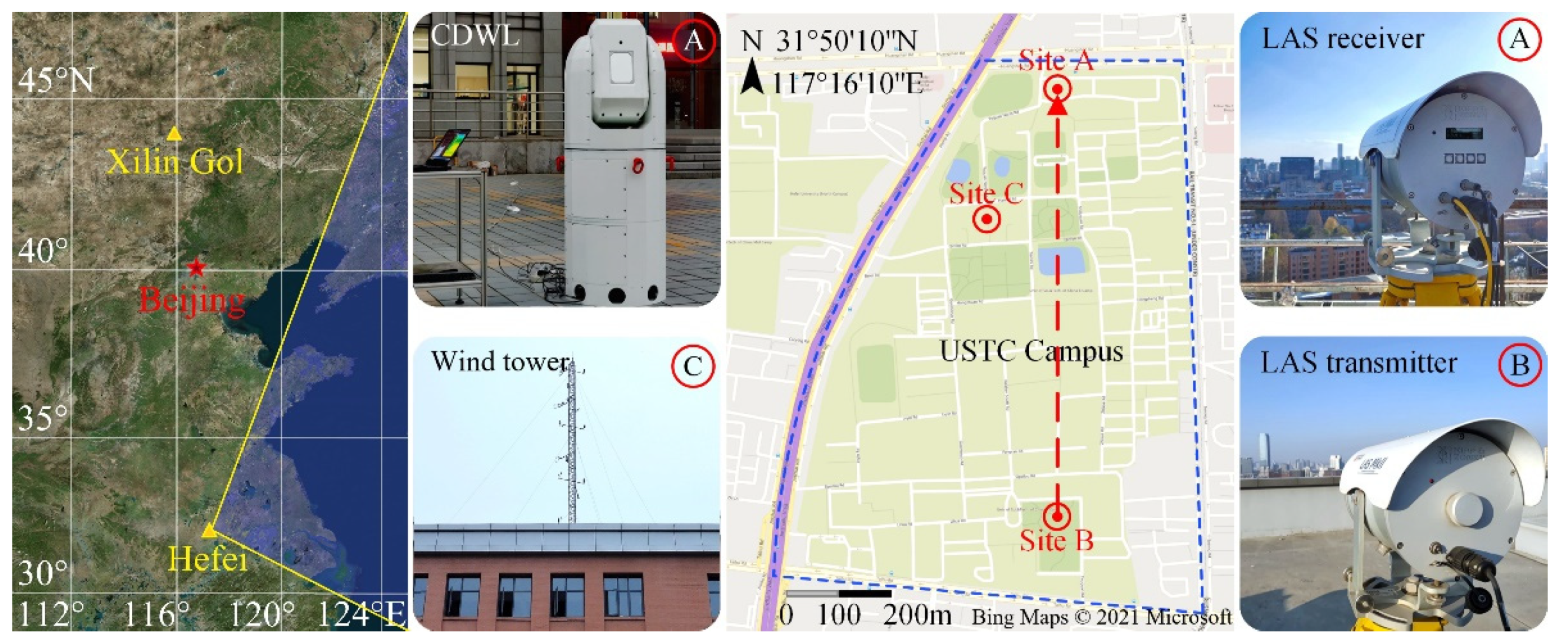
3.1. Instruments
3.2. Verification Experiment
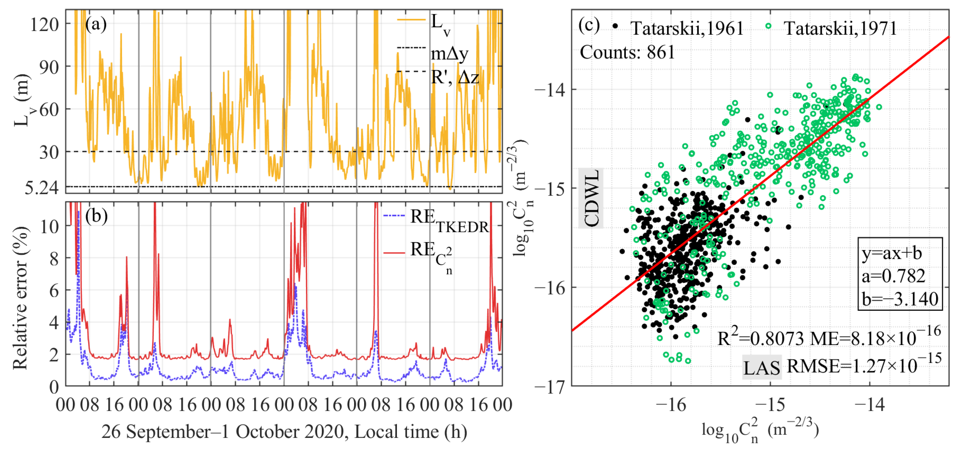
3.3. Limitation and Uncertainty Analysis
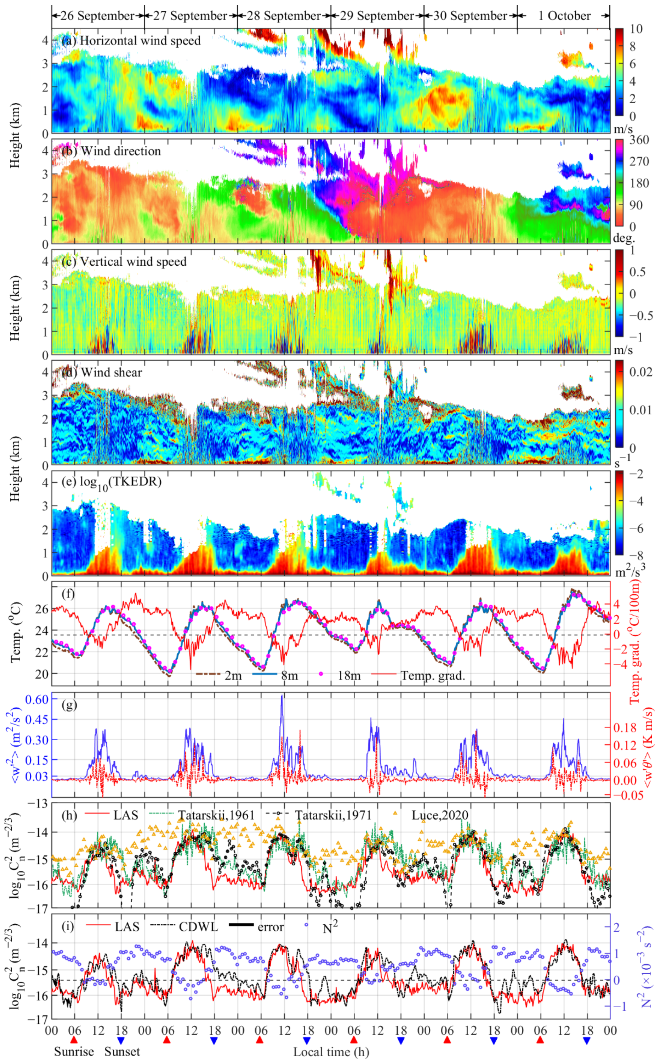
3.4. Continuous Observation of Profile
3.5. Results Analysis
4. Conclusions and Discussion
Author Contributions
Funding
Data Availability Statement
Acknowledgments
Conflicts of Interest
References
- Ma, B.; Shang, Z.; Hu, Y.; Hu, K.; Wang, Y.; Yang, X.; Ashley, M.C.B.; Hickson, P.; Jiang, P. Night-time measurements of astronomical seeing at Dome A in Antarctica. Nature 2020, 583, 771–774. [Google Scholar] [CrossRef] [PubMed]
- Storer, L.N.; Williams, P.D.; Gill, P.G. Aviation Turbulence: Dynamics, Forecasting, and Response to Climate Change. Pure Appl. Geophys. 2019, 176, 2081–2095. [Google Scholar] [CrossRef] [Green Version]
- Ren, Y.; Huang, H.; Xie, G.; Ahmed, N.; Yan, Y.; Erkmen, B.I.; Chandrasekaran, N.; Lavery, M.P.J.; Steinhoff, N.K.; Tur, M.; et al. Atmospheric turbulence effects on the performance of a free space optical link employing orbital angular momentum multiplexing. Opt. Lett. 2013, 38, 4062–4065. [Google Scholar] [CrossRef] [PubMed]
- Extance, A. Laser weapons get real. Nature 2015, 521, 408–410. [Google Scholar] [CrossRef] [PubMed] [Green Version]
- Kumer, V.-M.; Reuder, J.; Dorninger, M.; Zauner, R.; Grubsic, V. Turbulent kinetic energy estimates from profiling wind LiDAR measurements and their potential for wind energy applications. Renew. Energy 2016, 99, 898–910. [Google Scholar] [CrossRef] [Green Version]
- Wei, W.; Zhang, H.; Cai, X.; Song, Y.; Bian, Y.; Xiao, K.; Zhang, H. Influence of Intermittent Turbulence on Air Pollution and Its Dispersion in Winter 2016/2017 over Beijing, China. J. Meteorol. Res. 2020, 34, 176–188. [Google Scholar] [CrossRef]
- Nootz, G.; Jarosz, E.; Dalgleish, F.R.; Hou, W. Quantification of optical turbulence in the ocean and its effects on beam propagation. Appl. Opt. 2016, 55, 8813–8820. [Google Scholar] [CrossRef]
- Libich, J.; Perez, J.; Zvanovec, S.; Ghassemlooy, Z.; Nebuloni, R.; Capsoni, C. Combined effect of turbulence and aerosol on free-space optical links. Appl. Opt. 2017, 56, 336–341. [Google Scholar] [CrossRef]
- Butterley, T.; Wilson, R.W.; Sarazin, M. Determination of the profile of atmospheric optical turbulence strength from SLODAR data. Mon. Not. R. Astron. Soc. 2006, 369, 835–845. [Google Scholar] [CrossRef] [Green Version]
- Voyez, J.; Robert, C.; Conan, J.-M.; Mugnier, L.M.; Samain, E.; Ziad, A. First on-sky results of the CO-SLIDAR Cn2 profiler. Opt. Express 2014, 22, 10948–10967. [Google Scholar] [CrossRef] [Green Version]
- Fusco, T.; Costille, A. Impact of Cn2 profile structure on Wide Field AO performance. Adapt. Opt. Syst. II 2010, 7736. [Google Scholar] [CrossRef]
- Voyez, J.; Robert, C.; Michau, V.; Conan, J.-M.; Fusco, T. Accurate measurement of Cn2 profile with Shack-Hartmann data. Adapt. Opt. Syst. III 2010, 7736, 77360J. [Google Scholar] [CrossRef] [Green Version]
- Otoniel Canuet, L.F. Atmospheric Turbulence Profile Modeling for Satellite-Ground Laser Communication; UPC, Escola d’Enginyeria de Telecomunicació i Aeroespacial de Castelldefels: Barcelona, Spain, 2015. [Google Scholar]
- Beland, R.R. Propagation through Atmospheric Optical Turbulence; SPIE: New York, NY, USA, 1993. [Google Scholar]
- Andrews, L.C.; Phillips, R.L.; Wayne, D.; Leclerc, T.; Sauer, P.; Crabbs, R.; Kiriazes, J. Near-ground vertical profile of refractive-index fluctuations. Proc. SPIE—Int. Soc. Opt. Eng. 2009, 7324, 732402–732412. [Google Scholar] [CrossRef]
- Chen, X.; Li, X.; Sun, G.; Liu, Q.; Zhu, W.; Weng, N. Analysis of an optical turbulence profile using complete ensemble empirical mode decomposition. Appl. Opt. 2016, 55, 9932–9938. [Google Scholar] [CrossRef]
- Wu, S.; Wu, X.; Su, C.; Yang, Q.; Xu, J.; Luo, T.; Huang, C.; Qing, C. Reliable model to estimate the profile of the refractive index structure parameter (Cn2) and integrated astroclimatic parameters in the atmosphere. Opt. Express 2021, 29, 12454–12470. [Google Scholar] [CrossRef] [PubMed]
- Barletti, R.; Ceppatelli, G.; Moroder, E.; Paterno, L.; Righini, A. A vertical profile of turbulence in atlantic air mass measured by balloon-borne radiosondes. J. Geophys. Res. 1974, 79, 4545–4549. [Google Scholar] [CrossRef]
- Martini, E.; Freni, A.; Cuccoli, F.; Facheris, L. Derivation of clear-air turbulence parameters from high-resolution radiosonde data. J. Atmos. Ocean. Technol. 2017, 34, 277–293. [Google Scholar] [CrossRef]
- Zhang, J.; Zhang, S.D.; Huang, C.M.; Huang, K.M.; Gong, Y.; Gan, Q.; Zhang, Y.H. Latitudinal and topographical variabilities of free atmospheric turbulence from high-resolution radiosonde data sets. J. Geophys. Res. Atmos. 2019, 124, 4283–4298. [Google Scholar] [CrossRef]
- Ko, H.C.; Chun, H.Y.; Wilson, R.; Geller, M.A. Characteristics of atmospheric turbulence retrieved from high vertical-resolution radiosonde data in the United States. J. Geophys. Res. Atmos. 2019, 124, 7553–7579. [Google Scholar] [CrossRef]
- He, Y.; Sheng, Z.; He, M. The First Observation of Turbulence in Northwestern China by a Near-Space High-Resolution Balloon Sensor. Sensors 2020, 20, 677. [Google Scholar] [CrossRef] [Green Version]
- Vyhnalek, B.E. Path Profiles of Cn2 Derived from Radiometer Temperature Measurements and Geometrical Ray Tracing. In Free-Space Laser Communication and Atmospheric Propagation XXIX; SPIE: New York, NY, USA, 2017; Volume 10096. [Google Scholar] [CrossRef] [Green Version]
- van Iersel, M.; Paulson, D.A.; Wu, C.; Ferlic, N.A.; Rzasa, J.R.; Davis, C.C.; Walker, M.; Bowden, M.; Spychalsky, J.; Titus, F. Measuring the turbulence profile in the lower atmospheric boundary layer. Appl. Opt. 2019, 58, 6934–6941. [Google Scholar] [CrossRef] [PubMed]
- Odintsov, S.L.; Gladkikh, V.A.; Kamardin, A.P.; Nevzorova, I.V. Determination of the Structural Characteristic of the Refractive Index of Optical Waves in the Atmospheric Boundary Layer with Remote Acoustic Sounding Facilities. Atmosphere 2019, 10, 711. [Google Scholar] [CrossRef] [Green Version]
- Ting-i, W.; Ochs, G.R.; Clifford, S.F. A saturation-resistant optical scintillometer to measure Cn2. J. Opt. Soc. Am. 1978, 68, 334–338. [Google Scholar]
- Andrews, L.C.; Phillips, R.L.; Crabbs, R.; Wayne, D.; Leclerc, T.; Sauer, P. Creating a Cn2 Profile as a Function of Altitude Using Scintillation Measurements Along a Slant Path. In High Energy/Average Power Lasers and Intense Beam Applications VI Atmospheric and Oceanic Propagation of Electromagnetic Waves VI; SPIE: New York, NY, USA, 2012; Volume 8238. [Google Scholar] [CrossRef]
- Han, Y.; Gao, P.; Huang, J.; Zhang, T.; Zhuang, J.; Hu, M.; Wu, Y. Ground-based synchronous optical instrument for measuring atmospheric visibility and turbulence intensity: Theories, design and experiments. Opt. Express 2018, 26, 6833–6850. [Google Scholar] [CrossRef] [PubMed]
- Belen’kii, M.S.; Roberts, D.W.; Stewart, J.M.; Gimmestad, G.G.; Dagle, W.R. Experimental validation of the differential image motion lidar concept. Laser Radar Technol. Appl. VI 2001, 4377, 307–316. [Google Scholar] [CrossRef]
- Gimmestad, G.; Roberts, D.; Stewart, J.; Wood, J. Development of a lidar technique for profiling optical turbulence. Opt. Eng. 2012, 51, 101713. [Google Scholar] [CrossRef]
- Brown, D.M.; Juarez, J.C.; Brown, A.M. Laser differential image-motion monitor for characterization of turbulence during free-space optical communication tests. Appl. Opt. 2013, 52, 8402–8410. [Google Scholar] [CrossRef]
- Jing, X.; Hou, Z.; Wu, Y.; Qin, L.A.; He, F.; Tan, F. Development of a differential column image motion light detection and ranging for measuring turbulence profiles. Opt. Lett. 2013, 38, 3445–3447. [Google Scholar] [CrossRef]
- Cheng, Z.; Tan, F.; Jing, X.; He, F.; Qin, L.A.; Hou, Z. Retrieval of Cn2 profile from differential column image motion lidar using the regularization method. Chin. Opt. Lett. 2017, 15, 020101. [Google Scholar] [CrossRef]
- Aristidi, E.; Ziad, A.; Chabe, J.; Fantei-Caujolle, Y.; Renaud, C.; Giordano, C. A generalized differential image motion monitor. arXiv 2019, arXiv:1904.07093. [Google Scholar] [CrossRef]
- Chabe, J.; Aristidi, E.; Ziad, A.; Lanteri, H.; Fantei-Caujolle, Y.; Giordano, C.; Borgnino, J.; Marjani, M.; Renaud, C. PML: A generalized monitor of atmospheric turbulence profile with high vertical resolution. Appl. Opt. 2020, 59, 7574–7584. [Google Scholar] [CrossRef] [PubMed]
- Banakh, V.A.; Razenkov, I.A. Refractive turbulence strength estimation based on the laser echo signal amplification effect. Opt. Lett. 2016, 41, 4429–4432. [Google Scholar] [CrossRef]
- Banakh, V.A.; Razenkov, I.A. Lidar measurements of atmospheric backscattering amplification. Opt. Spectrosc. 2016, 120, 326–334. [Google Scholar] [CrossRef]
- Razenkov, I.A. Turbulent Lidar: II-Experiment. Atmos. Ocean. Opt. 2018, 31, 281–289. [Google Scholar] [CrossRef]
- Whiteman, D.N.; Venable, D.; Landulfo, E. Comments on “Accuracy of Raman lidar water vapor calibration and its applicability to long-term measurements”. Appl. Opt. 2011, 50, 2170–2176. [Google Scholar] [CrossRef] [Green Version]
- Shangguan, M.; Xia, H.; Wang, C.; Qiu, J.; Lin, S.; Dou, X.; Zhang, Q.; Pan, J.-W. Dual-frequency Doppler lidar for wind detection with a superconducting nanowire single-photon detector. Opt. Lett. 2017, 42, 3541–3544. [Google Scholar] [CrossRef] [PubMed]
- Wang, C.; Xia, H.; Wu, Y.; Dong, J.; Wei, T.; Wang, L.; Dou, X. Meter-scale spatial-resolution-coherent Doppler wind lidar based on Golay coding. Opt. Lett. 2019, 44, 311–314. [Google Scholar] [CrossRef] [PubMed] [Green Version]
- Zhang, Y.; Wu, Y.; Xia, H. Spatial resolution enhancement of coherent Doppler wind lidar using differential correlation pair technique. Opt. Lett. 2021, 46, 5550–5553. [Google Scholar] [CrossRef]
- Banakh, V.A.; Smalikho, I.N.; Falits, A.V. Estimation of the turbulence energy dissipation rate in the atmospheric boundary layer from measurements of the radial wind velocity by micropulse coherent Doppler lidar. Opt. Express 2017, 25, 22679–22692. [Google Scholar] [CrossRef]
- Banakh, V.A.; Smalikho, I.N.; Falits, A.V. Wind-Temperature Regime and Wind Turbulence in a Stable Boundary Layer of the Atmosphere: Case Study. Remote Sens. 2020, 12, 955. [Google Scholar] [CrossRef] [Green Version]
- Banakh, V.A.; Smalikho, I.N.; Falits, A.V. Estimation of the height of the turbulent mixing layer from data of Doppler lidar measurements using conical scanning by a probe beam. Atmos. Meas. Tech. 2021, 14, 1511–1524. [Google Scholar] [CrossRef]
- Smalikho, I.N.; Banakh, V.A. Effect of Wind Transport of Turbulent Inhomogeneities on Estimation of the Turbulence Energy Dissipation Rate from Measurements by a Conically Scanning Coherent Doppler Lidar. Remote Sens. 2020, 12, 2802. [Google Scholar] [CrossRef]
- Banakh, V.A.; Smalikho, I.N.; Falits, A.V.; Sherstobitov, A.M. Estimating the Parameters of Wind Turbulence from Spectra of Radial Velocity Measured by a Pulsed Doppler Lidar. Remote Sens. 2021, 13, 2071. [Google Scholar] [CrossRef]
- Smalikho, I.N.; Banakh, V.A.; Falits, A.V.; Sukharev, A.A. Experimental Study of Aircraft Wake Vortices on the Airfield of Tolmachevo Airport in 2018. Atmos. Ocean. Opt. 2020, 33, 124–133. [Google Scholar] [CrossRef]
- Wang, C.; Jia, M.; Xia, H.; Wu, Y.; Wei, T.; Shang, X.; Yang, C.; Xue, X.; Dou, X. Relationship analysis of PM2.5 and boundary layer height using an aerosol and turbulence detection lidar. Atmos. Meas. Tech. 2019, 12, 3303–3315. [Google Scholar] [CrossRef] [Green Version]
- Yang, Y.; Fan, S.; Wang, L.; Gao, Z.; Zhang, Y.; Zou, H.; Miao, S.; Li, Y.; Huang, M.; Yim, S.H.L.; et al. Diurnal Evolution of the Wintertime Boundary Layer in Urban Beijing, China: Insights from Doppler Lidar and a 325-m Meteorological Tower. Remote Sens. 2020, 12, 3935. [Google Scholar] [CrossRef]
- Wang, L.; Qiang, W.; Xia, H.; Wei, T.; Yuan, J.; Jiang, P. Robust Solution for Boundary Layer Height Detections with Coherent Doppler Wind Lidar. Adv. Atmos. Sci. 2021, 38, 1920–1928. [Google Scholar] [CrossRef]
- Yuan, J.; Wu, K.; Wei, T.; Wang, L.; Shu, Z.; Yang, Y.; Xia, H. Cloud Seeding Evidenced by Coherent Doppler Wind Lidar. Remote Sens. 2021, 13, 3815. [Google Scholar] [CrossRef]
- Jia, M.; Yuan, J.; Wang, C.; Xia, H.; Wu, Y.; Zhao, L.; Wei, T.; Wu, J.; Wang, L.; Gu, S.-Y.; et al. Long-lived high-frequency gravity waves in the atmospheric boundary layer: Observations and simulations. Atmos. Chem. Phys. 2019, 19, 15431–15446. [Google Scholar] [CrossRef] [Green Version]
- Cao, C.; Xinzhao, C.; Jian, Z.; Roberts, B.R.; Zhibin, Y.; Weichun, F.; Xian, L.; Smith, J.A. Lidar observations of persistent gravity waves with periods of 3-10 h in the Antarctic middle and upper atmosphere at McMurdo (77.83degS, 166.67degE). J. Geophys. Res. Space Phys. 2016, 121, 1483–1502. [Google Scholar] [CrossRef]
- Tuononen, M.; O’Connor, E.J.; Sinclair, V.A.; Vakkari, V. Low-Level Jets over Uto, Finland, Based on Doppler Lidar Observations. J. Appl. Meteorol. Climatol. 2017, 56, 2577–2594. [Google Scholar] [CrossRef]
- Banakh, V.A.; Smalikho, I.N. Lidar Studies of Wind Turbulence in the Stable Atmospheric Boundary Layer. Remote Sens. 2018, 10, 1219. [Google Scholar] [CrossRef] [Green Version]
- Wei, T.; Xia, H.; Hu, J.; Wang, C.; Shangguan, M.; Wang, L.; Jia, M.; Dou, X. Simultaneous wind and rainfall detection by power spectrum analysis using a VAD scanning coherent Doppler lidar. Opt. Express 2019, 27, 31235–31245. [Google Scholar] [CrossRef] [PubMed]
- Yuan, J.; Xia, H.; Wei, T.; Wang, L.; Yue, B.; Wu, Y. Identifying cloud, precipitation, windshear, and turbulence by deep analysis of the power spectrum of coherent Doppler wind lidar. Opt. Express 2020, 28, 37406–37418. [Google Scholar] [CrossRef] [PubMed]
- Wang, C.; Xia, H.; Shangguan, M.; Wu, Y.; Wang, L.; Zhao, L.; Qiu, J.; Zhang, R. 1.5 µm polarization coherent lidar incorporating time-division multiplexing. Opt. Express 2017, 25, 20663–20674. [Google Scholar] [CrossRef] [PubMed] [Green Version]
- Wei, T.; Xia, H.; Wu, Y.; Yuan, J.; Wang, C.; Dou, X. Inversion probability enhancement of all-fiber CDWL by noise modeling and robust fitting. Opt. Express 2020, 28, 29662–29675. [Google Scholar] [CrossRef] [PubMed]
- Pan, Y.; Zhang, S.; Li, Q.; Ma, L.; Jiang, S.; Lei, L.; Lyu, W.; Wang, Z. Analysis of convective instability data derived from a ground-based microwave radiometer before triggering operations for artificial lightning. Atmos. Res. 2020, 243, 105005. [Google Scholar] [CrossRef]
- Kolmogorov, A.N. A refinement of previous hypotheses concerning the local structure of turbulence in a viscous incompressible fluid at high reynolds number. J. Fluid Mech. 1962, 13, 82–85. [Google Scholar] [CrossRef] [Green Version]
- Tatarskii, V.I. Wave Propagation in a Turbulent Medium; McGraw-Hill: New York, NY, USA, 1961. [Google Scholar]
- Andrews, L.C.; Phillips, R.L. Laser Beam Propagation through Random Media; SPIE: New York, NY, USA, 2005. [Google Scholar]
- Han, Y.; Wu, X.; Luo, T.; Qing, C.; Yang, Q.; Jin, X.; Liu, N.; Wu, S.; Su, C. New Cn2 statistical model based on first radiosonde turbulence observation over Lhasa. J. Opt. Soc. Am. A—Opt. Image Sci. Vis. 2020, 37, 995–1001. [Google Scholar] [CrossRef]
- Coulman, C.E.; Vernin, J.; Coqueugniot, Y.; Caccia, J.L. Outer scale of turbulence appropriate to modeling refractive-index structure profiles. Appl. Opt. 1988, 27, 155–160. [Google Scholar] [CrossRef]
- Dewan, E.M.; Beland, R.; Brown, J. A Model for Cn2 (Optical Turbulence) Profiles Using Radiosonde Data; Directorate of Geophysics: Hanscom Air Force Base, MA, USA, 1993. [Google Scholar]
- Stull, R.B. An Introduction to Boundary Layer Meteorology; Springer Science & Business Media: Dordrecht, The Netherlands; Kluwer Academic: Alphen aan den Rijn, The Netherlands, 1988. [Google Scholar]
- Tatarskii, V.I. The Effects of the Turbulent Atmosphere on Wave Propagation; Israel Program for Scientific Translations: Jerusalem, Palestine, 1971. [Google Scholar]
- Venayagamoorthy, S.K.; Stretch, D.D. On the turbulent Prandtl number in homogeneous stably stratified turbulence. J. Fluid Mech. 2010, 644, 359–369. [Google Scholar] [CrossRef] [Green Version]
- Kantha, L.; Luce, H. Mixing Coefficient in Stably Stratified Flows. J. Phys. Oceanogr. 2018, 48, 2649–2665. [Google Scholar] [CrossRef]
- Li, D. Turbulent Prandtl number in the atmospheric boundary layer—where are we now? Atmos. Res. 2019, 216, 86–105. [Google Scholar] [CrossRef]
- Luce, H.; Kantha, L.; Hashiguchi, H.; Lawrence, D. Estimation of Turbulence Parameters in the Lower Troposphere from ShUREX (2016–2017) UAV Data. Atmosphere 2019, 10, 384. [Google Scholar] [CrossRef] [Green Version]
- Ghannam, K.; Duman, T.; Salesky, S.T.; Chamecki, M.; Katul, G. The non-local character of turbulence asymmetry in the convective atmospheric boundary layer. Q. J. R. Meteorol. Soc. 2017, 143, 494–507. [Google Scholar] [CrossRef]
- Deardorff, J.W. The Counter-Gradient Heat Flux in the Lower Atmosphere and in the Laboratory. J. Atmos. Sci. 1966, 23, 503–506. [Google Scholar] [CrossRef] [Green Version]
- Luce, H.; Kantha, L.; Hashiguchi, H.; Doddi, A.; Lawrence, D.; Yabuki, M. On the Relationship between the TKE Dissipation Rate and the Temperature Structure Function Parameter in the Convective Boundary Layer. J. Atmos. Sci. 2020, 77, 2311–2326. [Google Scholar] [CrossRef] [Green Version]
- DAVIS6162: Wireless Vantage Pro2 Plus Support Documents. Available online: https://cdn.shopify.com/s/files/1/0515/5992/3873/files/07395.234_Manual_VP2__RevZ_web.pdf?v=1647548782 (accessed on 16 June 2022).
- LAS MkII Scintillometer—Manual. Available online: https://www.kippzonen.com/Download/598/LAS-MkII-Scintillometer-Manual (accessed on 16 June 2022).
- Olofson, K.F.G.; Andersson, P.U.; Hallquist, M.; Ljungstrom, E.; Tang, L.; Chen, D.; Pettersson, J.B.C. Urban aerosol evolution and particle formation during wintertime temperature inversions. Atmos. Environ. 2009, 43, 340–346. [Google Scholar] [CrossRef]
- Guo, J.; Chen, X.; Su, T.; Liu, L.; Zheng, Y.; Chen, D.; Li, J.; Xu, H.; Lv, Y.; He, B.; et al. The Climatology of Lower Tropospheric Temperature Inversions in China from Radiosonde Measurements: Roles of Black Carbon, Local Meteorology, and Large-Scale Subsidence. J. Clim. 2020, 33, 9327–9350. [Google Scholar] [CrossRef]
- Sorbjan, Z.; Balsley, B.B. Microstructure of turbulence in the stably stratified boundary layer. Bound.-Layer Meteorol. 2008, 129, 191–210. [Google Scholar] [CrossRef] [Green Version]
- Friedrich, K.; Lundquist, J.K.; Aitken, M.; Kalina, E.A.; Marshall, R.F. Stability and turbulence in the atmospheric boundary layer: A comparison of remote sensing and tower observations. Geophys. Res. Lett. 2012, 39, L03801. [Google Scholar] [CrossRef] [Green Version]
- Balsley, B.B.; Lawrence, D.A.; Fritts, D.C.; Wang, L.; Wan, K.; Werne, J. Fine Structure, Instabilities, and Turbulence in the Lower Atmosphere: High-Resolution In Situ Slant-Path Measurements with the DataHawk UAV and Comparisons with Numerical Modeling. J. Atmos. Ocean. Technol. 2018, 35, 619–642. [Google Scholar] [CrossRef]
- Smalikho, I.N.; Banakh, V.A. Measurements of wind turbulence parameters by a conically scanning coherent Doppler lidar in the atmospheric boundary layer. Atmos. Meas. Tech. 2017, 10, 4191–4208. [Google Scholar] [CrossRef] [Green Version]
- Frehlich, R.; Hannon, S.M.; Henderson, S.W. Performance of a 2-µm Coherent Doppler Lidar for Wind Measurements. J. Atmos. Ocean. Technol. 1994, 11, 1517–1528. [Google Scholar] [CrossRef]
- Rye, B.J.; Hardesty, R.M. Discrete spectral peak estimation in incoherent backscatter heterodyne lidar. I. Spectral accumulation and the Cramer-Rao lower bound. IEEE Trans. Geosci. Remote Sens. 1993, 31, 16–27. [Google Scholar] [CrossRef]
- Rye, B.J.; Hardesty, R.M. Discrete spectral peak estimation in incoherent backscatter heterodyne lidar. II. Correlogram accumulation. IEEE Trans. Geosci. Remote Sens. 1993, 31, 28–35. [Google Scholar] [CrossRef]
- Venayagamoorthy, S.K.; Koseff, J.R. On the flux Richardson number in stably stratified turbulence. J. Fluid Mech. 2016, 798, R1. [Google Scholar] [CrossRef]
- Banakh, V.A.; Smalikho, I.N.; Falits, A.V. Remote Sensing of Stable Boundary Layer of Atmosphere. In EPJ Web of Conferences; EDP Sciences: Les Ulis, France, 2020; p. 06015. [Google Scholar]
- Miles, J.W. On the stability of heterogeneous shear flows. J. Fluid Mech. 1961, 10, 496–508. [Google Scholar] [CrossRef] [Green Version]
- Stull, R. An Introduction to Boundary Layer Meteorology; Kluwer Academic Publishers: Dordrecht, The Netherlands, 1998; p. 176. [Google Scholar]
- Xu, G.; Xi, B.; Zhang, W.; Cui, C.; Dong, X.; Liu, Y.; Yan, G. Comparison of atmospheric profiles between microwave radiometer retrievals and radiosonde soundings. J. Geophys. Res. 2015, 120, 10313–10323. [Google Scholar] [CrossRef]
- Andrews, L.C.; Phillips, R.L.; Crabbs, R.; Wayne, D.; Leclerc, T.; Sauer, P. Atmospheric Channel Characterization for ORCA Testing at NTTR. In Atmospheric and Oceanic Propagation of Electromagnetic Waves IV; Korotkova, O., Ed.; SPIE: New York, NY, USA, 2010; Volume 7588. [Google Scholar]


| Parameter | Value |
|---|---|
| Wavelength | 1548 nm |
| Pulse energy | 200 μJ |
| Pulse width | 200 ns |
| Repetition frequency | 10 kHz |
| Temporal resolution | 2 s |
| Azimuth scanning range | 0–360° |
| Zenith scanning range | 0–90° |
Publisher’s Note: MDPI stays neutral with regard to jurisdictional claims in published maps and institutional affiliations. |
© 2022 by the authors. Licensee MDPI, Basel, Switzerland. This article is an open access article distributed under the terms and conditions of the Creative Commons Attribution (CC BY) license (https://creativecommons.org/licenses/by/4.0/).
Share and Cite
Jiang, P.; Yuan, J.; Wu, K.; Wang, L.; Xia, H. Turbulence Detection in the Atmospheric Boundary Layer Using Coherent Doppler Wind Lidar and Microwave Radiometer. Remote Sens. 2022, 14, 2951. https://doi.org/10.3390/rs14122951
Jiang P, Yuan J, Wu K, Wang L, Xia H. Turbulence Detection in the Atmospheric Boundary Layer Using Coherent Doppler Wind Lidar and Microwave Radiometer. Remote Sensing. 2022; 14(12):2951. https://doi.org/10.3390/rs14122951
Chicago/Turabian StyleJiang, Pu, Jinlong Yuan, Kenan Wu, Lu Wang, and Haiyun Xia. 2022. "Turbulence Detection in the Atmospheric Boundary Layer Using Coherent Doppler Wind Lidar and Microwave Radiometer" Remote Sensing 14, no. 12: 2951. https://doi.org/10.3390/rs14122951