
Wide and Deep Fourier Neural Network for Hyperspectral Remote Sensing Image Classification

 , , , , and
Abstract
:
1. Introduction
- Learning both spectral and spatial fine grained features efficiently using a large number of Fourier transforms in the wide direction, with computational load reduced by using pruning and retaining most effective features;
- Extracting hierarchical abstract features layer-by-layer in the deep direction with wide Fourier layers efficiently with limited training samples for HSI classification;
- Learning the weights in the fully connected layer by using least squares, which makes the training process very simple for HSI classification.
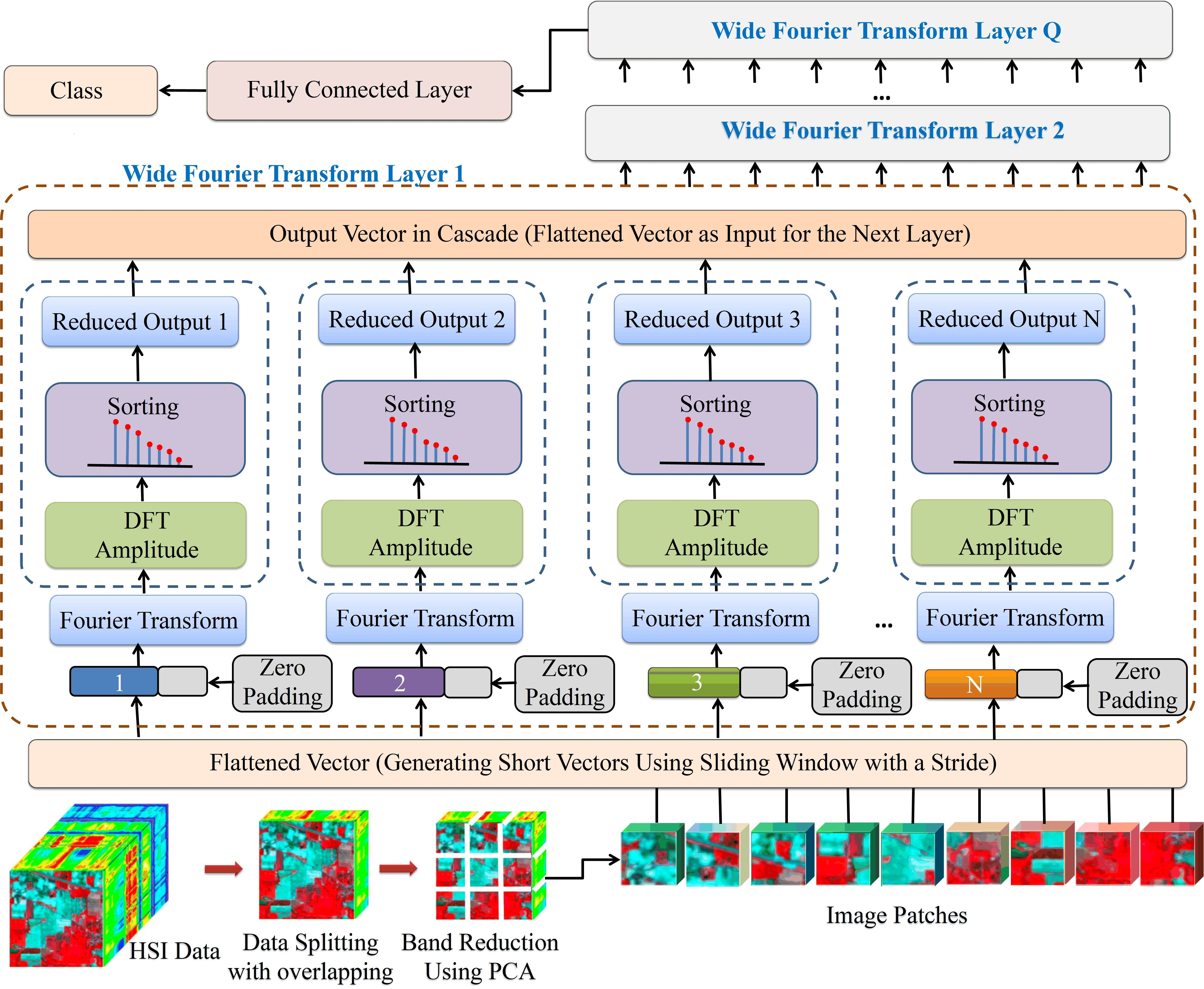
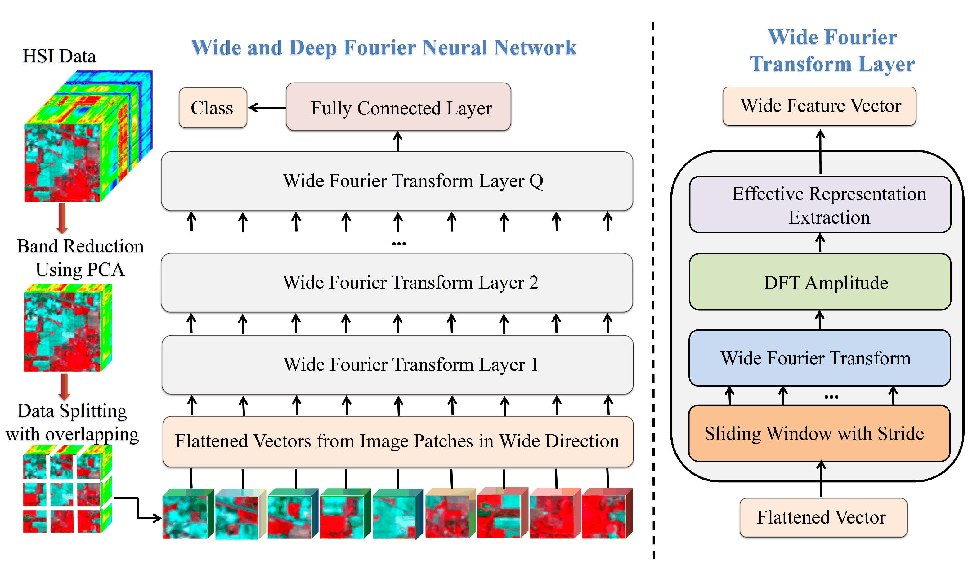
2. Wide and Deep Fourier Neural Network for Hyperspectral Image Classification
2.1. Hyperspectral Remote Sensing Data Sliptting
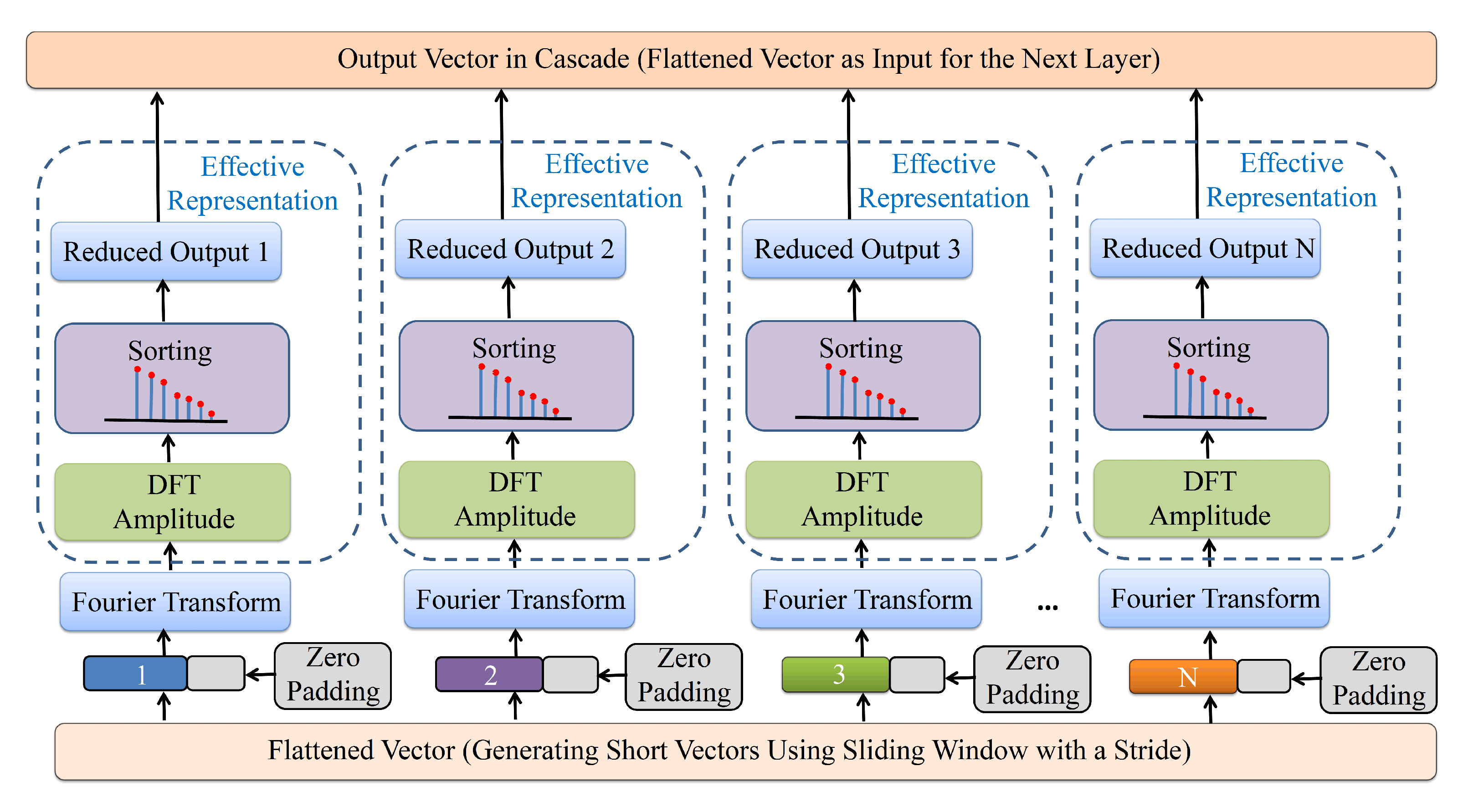
2.2. The Wide Fourier Transform Layer
2.3. Wide and Deep Fourier Neural Network
3. Datasets and Experimental Settings
3.1. Experimental Datasets
3.2. Experimental Setup
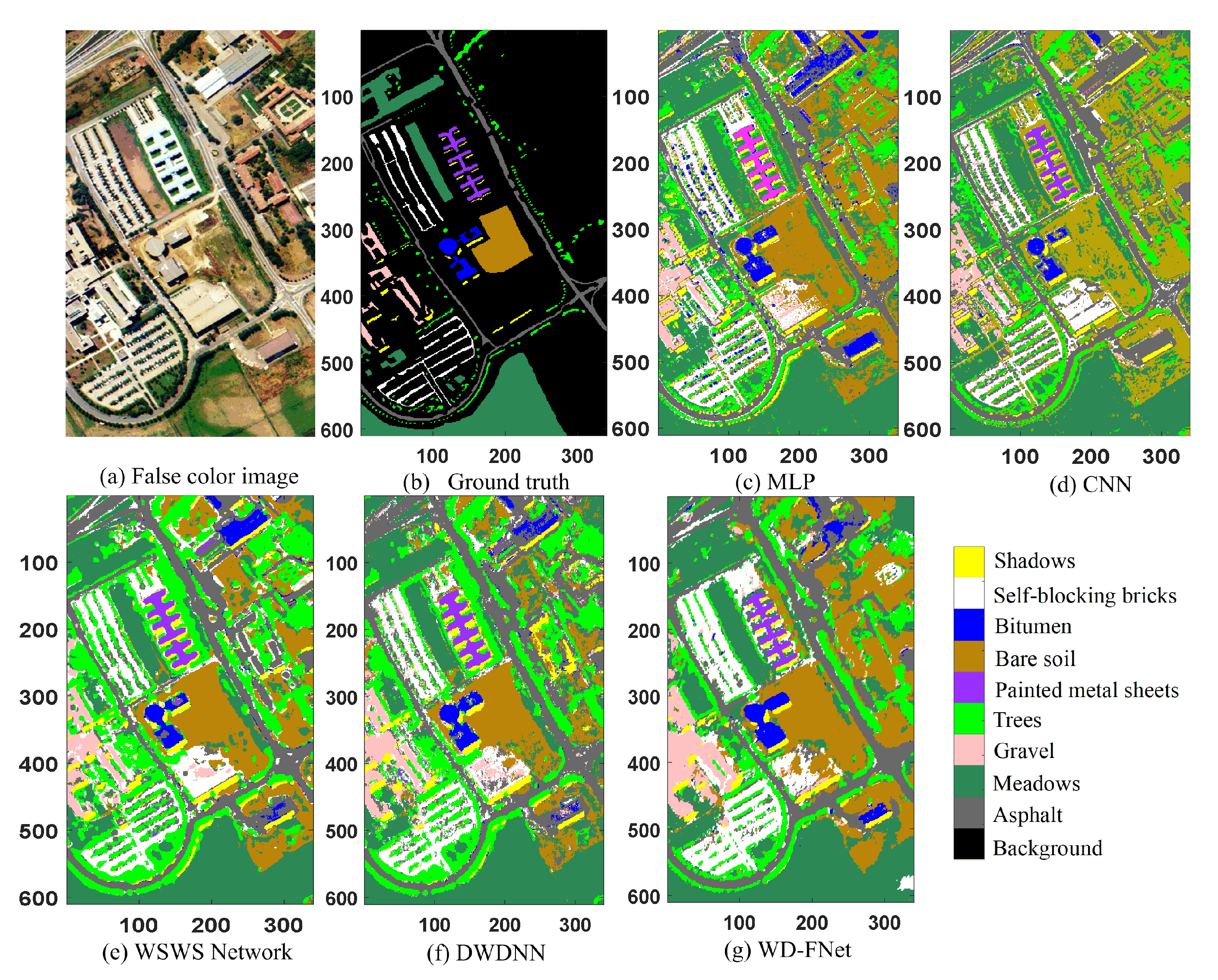
4. Experimental Results
Classification Performance on Different Datasets
5. Discussion
5.1. Effects of Different Sizes of Image Patches
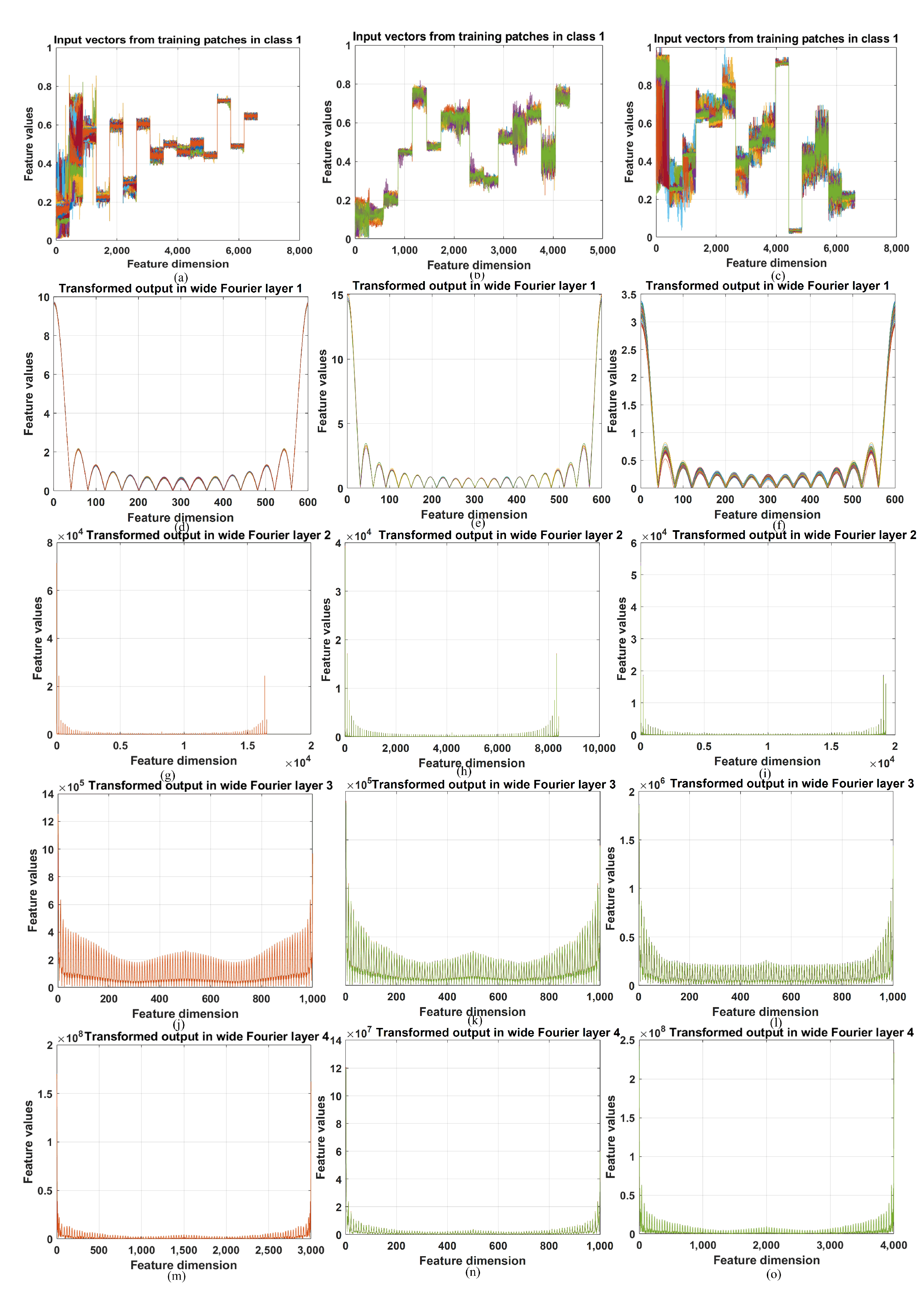
5.2. Visualization of the Fourier Transform Layers of the Wd-Fnet
5.3. Advantages and Limitations of the WD-Fnet Compared with Other Learning Models
6. Conclusions
Author Contributions
Funding
Data Availability Statement
Acknowledgments
Conflicts of Interest
Abbreviations
| HSI | Hyperspectral Image |
| PCA | Principal component analysis |
| DFT | Discrete Fourier transform |
| FFT | Fast Fourier transform |
| PCA | Principal component analysis |
| MLP | Multilayer perceptron |
| CNN | Convolutional neural network |
| LSTM | Long short-term memory |
| FCN | Fully convolutional network |
| GAN | Generative adversarial network |
| EWC | Elastic weight consolidation |
| PSHNN | Parallel, self-organizing, hierarchical neural networks |
| PCNN | D-parallel consensual neural networks |
| WSWS | Wide sliding window and subsampling |
| SWNN | Scalable wide neural network |
| DWDNN | Dynamic Wide and Deep Neural Network |
| WF | Wide Fourier |
| WD-FNet | Wide and Deep Fourier Neural Network |
| OA | Overall Accuracy |
| AA | Average Accuracy |
References
- Safavian, S.R.; Landgrebe, D. A survey of decision tree classifier methodology. IEEE Trans. Syst. Man Cybern. 1991, 21, 660–674. [Google Scholar] [CrossRef] [Green Version]
- Tarabalka, Y.; Fauvel, M.; Chanussot, J.; Benediktsson, J.A. SVM-and MRF-based method for accurate classification of hyperspectral images. IEEE Geosci. Remote Sens. Lett. 2010, 7, 736–740. [Google Scholar] [CrossRef] [Green Version]
- Xi, J.; Ersoy, O.K.; Fang, J.; Wu, T.; Wei, X.; Zhao, C. Parallel Multistage Wide Neural Network. IEEE Trans. Neural Netw. Learn. Syst. 2021, 1–14. [Google Scholar] [CrossRef] [PubMed]
- Li, J.; Bioucas-Dias, J.M.; Plaza, A. Semisupervised hyperspectral image classification using soft sparse multinomial logistic regression. IEEE Geosci. Remote Sens. Lett. 2012, 10, 318–322. [Google Scholar]
- Lee, H.; Kwon, H. Going deeper with contextual CNN for hyperspectral image classification. IEEE Trans. Image Process. 2017, 26, 4843–4855. [Google Scholar] [CrossRef] [PubMed] [Green Version]
- Zhang, L.; Zhang, L.; Du, B. Deep learning for remote sensing data: A technical tutorial on the state of the art. IEEE Geosci. Remote Sens. Mag. 2016, 4, 22–40. [Google Scholar] [CrossRef]
- Zhang, M.; Li, W.; Du, Q. Diverse region-based CNN for hyperspectral image classification. IEEE Trans. Image Process. 2018, 27, 2623–2634. [Google Scholar] [CrossRef]
- Wang, W.; Dou, S.; Jiang, Z.; Sun, L. A fast dense spectral–spatial convolution network framework for hyperspectral images classification. Remote Sens. 2018, 10, 1068. [Google Scholar] [CrossRef] [Green Version]
- Gong, Z.; Zhong, P.; Yu, Y.; Hu, W.; Li, S. A CNN with Multiscale Convolution and Diversified Metric for Hyperspectral Image Classification. IEEE Trans. Geosci. Remote Sens. 2019, 57, 3599–3618. [Google Scholar] [CrossRef]
- Gao, Q.; Lim, S.; Jia, X. Hyperspectral image classification using convolutional neural networks and multiple feature learning. Remote Sens. 2018, 10, 299. [Google Scholar] [CrossRef] [Green Version]
- Cheng, G.; Li, Z.; Han, J.; Yao, X.; Guo, L. Exploring hierarchical convolutional features for hyperspectral image classification. IEEE Trans. Geosci. Remote Sens. 2018, 56, 6712–6722. [Google Scholar] [CrossRef]
- Paoletti, M.; Haut, J.; Plaza, J.; Plaza, A. A new deep convolutional neural network for fast hyperspectral image classification. ISPRS J. Photogramm. Remote Sens. 2018, 145, 120–147. [Google Scholar] [CrossRef]
- Roy, S.K.; Krishna, G.; Dubey, S.R.; Chaudhuri, B.B. HybridSN: Exploring 3-D–2-D CNN feature hierarchy for hyperspectral image classification. IEEE Geosci. Remote Sens. Lett. 2019, 17, 277–281. [Google Scholar] [CrossRef] [Green Version]
- Zheng, J.; Feng, Y.; Bai, C.; Zhang, J. Hyperspectral Image Classification Using Mixed Convolutions and Covariance Pooling. IEEE Trans. Geosci. Remote Sens. 2020, 59, 522–534. [Google Scholar] [CrossRef]
- Shi, C.; Liao, D.; Zhang, T.; Wang, L. Hyperspectral Image Classification Based on Expansion Convolution Network. IEEE Trans. Geosci. Remote Sens. 2022, 60, 1–16. [Google Scholar] [CrossRef]
- Haut, J.M.; Paoletti, M.E.; Plaza, J.; Li, J.; Plaza, A. Active Learning With Convolutional Neural Networks for Hyperspectral Image Classification Using a New Bayesian Approach. IEEE Trans. Geosci. Remote Sens. 2018, 56, 6440–6461. [Google Scholar] [CrossRef]
- Tang, X.; Meng, F.; Zhang, X.; Cheung, Y.; Ma, J.; Liu, F.; Jiao, L. Hyperspectral Image Classification Based on 3-D Octave Convolution with Spatial-Spectral Attention Network. IEEE Trans. Geosci. Remote Sens. 2020, 59, 2430–2447. [Google Scholar] [CrossRef]
- Cao, X.; Yao, J.; Xu, Z.; Meng, D. Hyperspectral image classification with convolutional neural network and active learning. IEEE Trans. Geosci. Remote Sens. 2020, 58, 4604–4616. [Google Scholar] [CrossRef]
- Xie, F.; Gao, Q.; Jin, C.; Zhao, F. Hyperspectral image classification based on superpixel pooling convolutional neural network with transfer learning. Remote Sens. 2021, 13, 930. [Google Scholar] [CrossRef]
- Masarczyk, W.; Głomb, P.; Grabowski, B.; Ostaszewski, M. Effective Training of Deep Convolutional Neural Networks for Hyperspectral Image Classification through Artificial Labeling. Remote Sens. 2020, 12, 2653. [Google Scholar] [CrossRef]
- Mou, L.; Ghamisi, P.; Zhu, X.X. Deep recurrent neural networks for hyperspectral image classification. IEEE Trans. Geosci. Remote Sens. 2017, 55, 3639–3655. [Google Scholar] [CrossRef] [Green Version]
- Hang, R.; Liu, Q.; Hong, D.; Ghamisi, P. Cascaded recurrent neural networks for hyperspectral image classification. IEEE Trans. Geosci. Remote Sens. 2019, 57, 5384–5394. [Google Scholar] [CrossRef] [Green Version]
- Liu, Q.; Zhou, F.; Hang, R.; Yuan, X. Bidirectional-convolutional LSTM based spectral-spatial feature learning for hyperspectral image classification. Remote Sens. 2017, 9, 1330. [Google Scholar] [CrossRef] [Green Version]
- Mei, S.; Li, X.; Liu, X.; Cai, H.; Du, Q. Hyperspectral Image Classification Using Attention-Based Bidirectional Long Short-Term Memory Network. IEEE Trans. Geosci. Remote Sens. 2021, 60, 1–12. [Google Scholar] [CrossRef]
- Song, T.; Wang, Y.; Gao, C.; Chen, H.; Li, J. MSLAN: A Two-Branch Multidirectional Spectral–Spatial LSTM Attention Network for Hyperspectral Image Classification. IEEE Trans. Geosci. Remote Sens. 2022, 60, 1–14. [Google Scholar] [CrossRef]
- He, X.; Chen, Y.; Lin, Z. Spatial-Spectral Transformer for Hyperspectral Image Classification. Remote Sens. 2021, 13, 498. [Google Scholar] [CrossRef]
- Qing, Y.; Liu, W.; Feng, L.; Gao, W. Improved Transformer Net for Hyperspectral Image Classification. Remote Sens. 2021, 13, 2216. [Google Scholar] [CrossRef]
- Zhou, F.; Hang, R.; Li, J.; Zhang, X.; Xu, C. Spectral-Spatial Correlation Exploration for Hyperspectral Image Classification via Self-Mutual Attention Network. IEEE Geosci. Remote Sens. Lett. 2022, 19, 1–5. [Google Scholar] [CrossRef]
- Lin, J.; Ma, L.; Yao, Y. A Fourier domain acceleration framework for convolutional neural networks. Neurocomputing 2019, 364, 254–268. [Google Scholar] [CrossRef]
- Ayat, S.O.; Khalil-Hani, M.; Ab Rahman, A.A.H.; Abdellatef, H. Spectral-based convolutional neural network without multiple spatial-frequency domain switchings. Neurocomputing 2019, 364, 152–167. [Google Scholar] [CrossRef]
- Khan, S.H.; Hayat, M.; Porikli, F. Regularization of deep neural networks with spectral dropout. Neural Netw. 2019, 110, 82–90. [Google Scholar] [CrossRef] [PubMed] [Green Version]
- Uteuliyeva, M.; Zhumekenov, A.; Takhanov, R.; Assylbekov, Z.; Castro, A.J.; Kabdolov, O. Fourier neural networks: A comparative study. Intell. Data Anal. 2020, 24, 1107–1120. [Google Scholar] [CrossRef]
- Silvescu, A. Fourier neural networks. In Proceedings of the IJCNN’99 International Joint Conference on Neural Networks, Washington, DC, USA, 10–16 July 1999; IEEE: Piscataway, NJ, USA, 1999; Volume 1, pp. 488–491. [Google Scholar]
- Li, Z.; Kovachki, N.B.; Azizzadenesheli, K.; Bhattacharya, K.; Stuart, A.; Anandkumar, A. Fourier Neural Operator for Parametric Partial Differential Equations. In Proceedings of the International Conference on Learning Representations, Addis Ababa, Ethiopia, 26–30 April 2020. [Google Scholar]
- Rao, Y.; Zhao, W.; Zhu, Z.; Lu, J.; Zhou, J. Global filter networks for image classification. Adv. Neural Inf. Process. Syst. 2021, 34, 980–993. [Google Scholar]
- Worrall, D.E.; Garbin, S.J.; Turmukhambetov, D.; Brostow, G.J. Harmonic networks: Deep translation and rotation equivariance. In Proceedings of the IEEE Conference on Computer Vision and Pattern Recognition, Honolulu, HI, USA, 21–26 July 2017; pp. 5028–5037. [Google Scholar]
- Liu, C.; Li, J.; He, L.; Plaza, A.; Li, S.; Li, B. Naive Gabor Networks for Hyperspectral Image Classification. IEEE Trans. Neural Netw. Learn. Syst. 2020, 32, 376–390. [Google Scholar] [CrossRef] [PubMed] [Green Version]
- Okwuashi, O.; Ndehedehe, C.E. Deep support vector machine for hyperspectral image classification. Pattern Recognit. 2020, 103, 107298. [Google Scholar] [CrossRef]
- Roy, S.K.; Haut, J.M.; Paoletti, M.E.; Dubey, S.R.; Plaza, A. Generative Adversarial Minority Oversampling for Spectral-Spatial Hyperspectral Image Classification. IEEE Trans. Geosci. Remote Sens. 2021, 60, 1–15. [Google Scholar] [CrossRef]
- Liang, H.; Bao, W.; Shen, X.; Zhang, X. Spectral-Spatial Attention Feature Extraction for Hyperspectral Image Classification Based on Generative Adversarial Network. IEEE J. Sel. Top. Appl. Earth Obs. Remote Sens. 2021, 14, 10017–10032. [Google Scholar] [CrossRef]
- Parisi, G.I.; Kemker, R.; Part, J.L.; Kanan, C.; Wermter, S. Continual lifelong learning with neural networks: A review. Neural Netw. 2019, 113, 54–71. [Google Scholar] [CrossRef]
- Venkataramani, S.; Raghunathan, A.; Liu, J.; Shoaib, M. Scalable-effort classifiers for energy-efficient machine learning. In Proceedings of the 52nd Annual Design Automation Conference, San Francisco, CA, USA, 8–12 June 2015; ACM: New York, NY, USA, 2015; p. 67. [Google Scholar]
- Panda, P.; Venkataramani, S.; Sengupta, A.; Raghunathan, A.; Roy, K. Energy-Efficient Object Detection Using Semantic Decomposition. IEEE Trans. Very Large Scale Integr. (VLSI) Syst. 2017, 25, 2673–2677. [Google Scholar] [CrossRef]
- Kirkpatrick, J.; Pascanu, R.; Rabinowitz, N.; Veness, J.; Desjardins, G.; Rusu, A.A.; Milan, K.; Quan, J.; Ramalho, T.; Grabska-Barwinska, A. Overcoming catastrophic forgetting in neural networks. Proc. Natl. Acad. Sci. USA 2017, 114, 3521–3526. [Google Scholar] [CrossRef] [Green Version]
- Lee, S.W.; Kim, J.H.; Jun, J.; Ha, J.W.; Zhang, B.T. Overcoming catastrophic forgetting by incremental moment matching. Adv. Neural Inf. Process. Syst. 2017, 30, 4652–4662. [Google Scholar]
- Ersoy, O.K.; Hong, D. Parallel, self-organizing, hierarchical neural networks. IEEE Trans. Neural Netw. 1990, 1, 167–178. [Google Scholar] [CrossRef] [PubMed] [Green Version]
- Benediktsson, J.A.; Sveinsson, J.R.; Ersoy, O.K.; Swain, P.H. Parallel consensual neural networks. IEEE Trans. Neural Netw. 1997, 8, 54–64. [Google Scholar] [CrossRef] [Green Version]
- Neyshabur, B.; Li, Z.; Bhojanapalli, S.; LeCun, Y.; Srebro, N. The role of over-parametrization in generalization of neural networks. In Proceedings of the International Conference on Learning Representations, New Orleans, LA, USA, 6–9 May 2019. [Google Scholar]
- Lee, J.; Xiao, L.; Schoenholz, S.S.; Bahri, Y.; Sohl-Dickstein, J.; Pennington, J. Wide neural networks of any depth evolve as linear models under gradient descent. arXiv 2019, arXiv:1902.06720. [Google Scholar] [CrossRef]
- Cheng, H.T.; Koc, L.; Harmsen, J.; Shaked, T.; Chandra, T.; Aradhye, H.; Anderson, G.; Corrado, G.; Chai, W.; Ispir, M. Wide & deep learning for recommender systems. In Proceedings of the 1st Workshop on Deep Learning for Recommender Systems, Boston, MA, USA, 15 September 2016; ACM: New York, NY, USA, 2016; pp. 7–10. [Google Scholar]
- Liu, W.; Nie, X.; Zhang, B.; Sun, X. Incremental Learning with Open-Set Recognition for Remote Sensing Image Scene Classification. IEEE Trans. Geosci. Remote Sens. 2022, 60, 1–16. [Google Scholar] [CrossRef]
- Xi, J.; Ersoy, O.K.; Fang, J.; Cong, M.; Wei, X.; Wu, T. Scalable Wide Neural Network: A Parallel, Incremental Learning Model Using Splitting Iterative Least Squares. IEEE Access 2021, 9, 50767–50781. [Google Scholar] [CrossRef]
- Xi, J.; Ersoy, O.K.; Fang, J.; Cong, M.; Wu, T.; Zhao, C.; Li, Z. Wide Sliding Window and Subsampling Network for Hyperspectral Image Classification. Remote Sens. 2021, 13, 1290. [Google Scholar] [CrossRef]
- Xi, J.; Cong, M.; Ersoy, O.K.; Zou, W.; Zhao, C.; Li, Z.; Gu, J.; Wu, T. Dynamic Wide and Deep Neural Network for Hyperspectral Image Classification. Remote Sens. 2021, 13, 2575. [Google Scholar] [CrossRef]
- Azar, S.G.; Meshgini, S.; Rezaii, T.Y.; Beheshti, S. Hyperspectral image classification based on sparse modeling of spectral blocks. Neurocomputing 2020, 407, 12–23. [Google Scholar] [CrossRef]
- Cheng, C.; Li, H.; Peng, J.; Cui, W.; Zhang, L. Deep High Order Tensor Convolutional Sparse Coding for Hyperspectral Image Classification. IEEE Trans. Geosci. Remote Sens. 2022, 60, 1–11. [Google Scholar] [CrossRef]
- Cheng, C.; Li, H.; Peng, J.; Cui, W.; Zhang, L. Hyperspectral Image Classification Via Spectral-Spatial Random Patches Network. IEEE J. Sel. Top. Appl. Earth Obs. Remote Sens. 2021, 14, 4753–4764. [Google Scholar] [CrossRef]
- Li, Z.; Wang, T.; Li, W.; Du, Q.; Wang, C.; Liu, C.; Shi, X. Deep Multilayer Fusion Dense Network for Hyperspectral Image Classification. IEEE J. Sel. Top. Appl. Earth Obs. Remote Sens. 2020, 13, 1258–1270. [Google Scholar] [CrossRef]


| Dataset | Description |
|---|---|
| Pavia University | It was acquired by the Reflective Optics System Imaging Spectrometer (ROSIS) sensor over the Pavia University campus. It has nine classes of land cover. The image dimension is . After discarding the pixels without information, the dimension is with 103 spectral bands. |
| KSC | The Kennedy Space Center (KSC, Merritt Island, FL, USA) dataset was acquired over the Kennedy Space Center in Florida. The image size is , and there are 13 classes of land cover. It has 176 bands after removing water absorption and low SNR bands. |
| Salinas | It was acquired in Salinas valley, California. The image size is pixels, and the number of classes is 16. There are 204 bands after removing bands of water absorption. |
| Class NO. | Pavia University | KSC | Salinas | |||
|---|---|---|---|---|---|---|
| Land Cover Class | NO. | Land Cover Class | NO. | Land Cover Class | NO. | |
| 1 | Asphalt | 6631 | Scrub | 347 | Brocoli-green-weeds-1 | 2009 |
| 2 | Meadows | 18,649 | Willow swamp | 243 | Brocoli-green-weeds-2 | 3726 |
| 3 | Gravel | 2099 | CP hammock | 256 | Fallow | 1976 |
| 4 | Trees | 3064 | Slash pine | 252 | Fallow-rough-plow | 1394 |
| 5 | Painted metal sheets | 1345 | Oak/broadleaf | 161 | Fallow-smooth | 2678 |
| 6 | Bare soil | 5029 | Hardwood | 229 | Stubble | 3959 |
| 7 | Bitumen | 1330 | Swamp | 105 | Celery | 3579 |
| 8 | Self-blocking bricks | 3682 | Graminoid marsh | 390 | Grapes-untrained | 11,271 |
| 9 | Shadows | 947 | Spartina marsh | 520 | Soil-vinyard-develop | 6203 |
| 10 | Cattail marsh | 404 | Corn-senesced-green-weeds | 3278 | ||
| 11 | Salt marsh | 419 | Lettuce-romaine-4wk | 1068 | ||
| 12 | Mud flats | 503 | Lettuce-romaine-5wk | 1927 | ||
| 13 | Water | 927 | Lettuce-romaine-6wk | 916 | ||
| 14 | Lettuce-romaine-7wk | 1070 | ||||
| 15 | Vinyard-untrained | 7268 | ||||
| 16 | Vinyard-vertica-trellis | 1807 | ||||
| Total | 42,776 | 5211 | 54,129 | |||
| Dataset | Hyperparameters of the WD-FNet for Different Datasets | |||||||
|---|---|---|---|---|---|---|---|---|
| Pavia University | Wide Fourier Layer 1 | Wide Fourier Layer 2 | ||||||
| Window | Stride | DFT Pts. | Pruned NO. | Window | Stride | DFT Pts. | Pruned NO. | |
| 15 | 0.9 | 600 | 100 | 0.35 | 0.15 | 1000 | 100 | |
| Wide Fourier Layer 3 | Wide Fourier Layer 4 | |||||||
| Window | Stride | DFT Pts. | Pruned NO. | Window | Stride | DFT Pts. | Pruned NO. | |
| 0.3 | 0.15 | 1000 | 100 | 0.32 | 0.15 | 3000 | 300 | |
| KSC | Wide Fourier Layer 1 | Wide Fourier Layer 2 | ||||||
| Window | Stride | DFT Pts. | Pruned NO. | Window | Stride | DFT Pts. | Pruned NO. | |
| 20 | 0.9 | 600 | 100 | 0.35 | 0.15 | 1000 | 100 | |
| Wide Fourier Layer 3 | Wide Fourier Layer 4 | |||||||
| Window | Stride | DFT Pts. | Pruned NO. | Window | Stride | DFT Pts. | Pruned NO. | |
| 0.3 | 0.15 | 1000 | 100 | 0.37 | 0.15 | 1000 | 50 | |
| Salinas | Wide Fourier Layer 1 | Wide Fourier Layer 2 | ||||||
| Window | Stride | DFT Pts. | Pruned NO. | Window | Stride | DFT Pts. | Pruned NO. | |
| 15 | 0.8 | 600 | 100 | 1.35 | 0.15 | 1000 | 100 | |
| Wide Fourier Layer 3 | Wide Fourier Layer 4 | |||||||
| Window | Stride | DFT Pts. | Pruned NO. | Window | Stride | DFT Pts. | Pruned NO. | |
| 0.5 | 0.15 | 1000 | 100 | 0.37 | 0.15 | 4000 | 400 | |
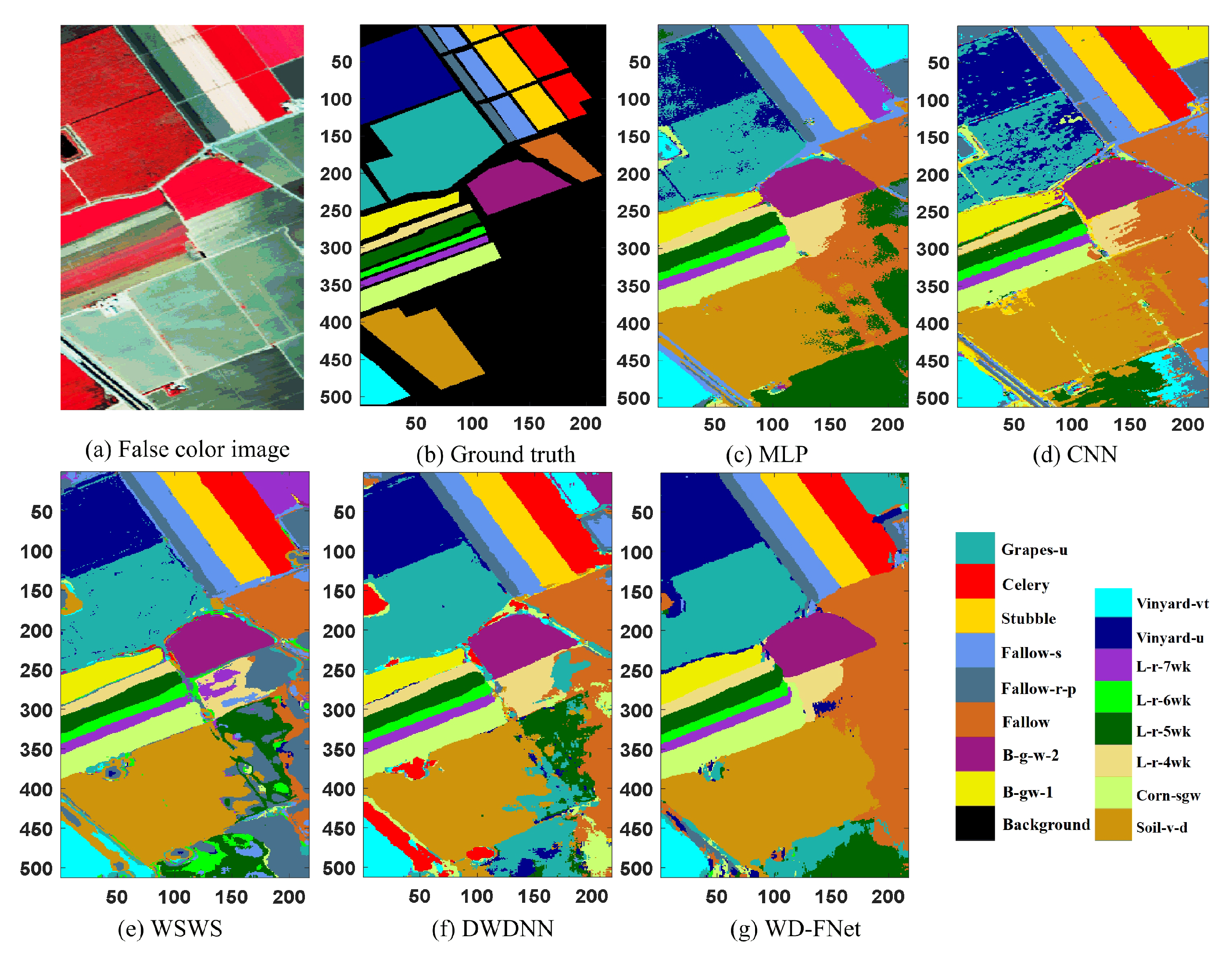
| Class NO. | MLP | CNN | 2-D CNN | 3-D CNN | SMSB | WSWS | DWDNN | WD-FNet |
|---|---|---|---|---|---|---|---|---|
| 1 | 97.13 | 96.18 | 98.51 | 98.40 | 99.11 | 99.10 | 99.87 | 99.85 |
| 2 | 98.43 | 96.69 | 99.54 | 96.91 | 98.97 | 100.00 | 100.00 | 99.96 |
| 3 | 85.15 | 80.86 | 84.62 | 97.05 | 98.89 | 93.01 | 96.98 | 98.89 |
| 4 | 95.05 | 87.21 | 98.04 | 98.84 | 98.74 | 98.37 | 99.29 | 99.18 |
| 5 | 99.88 | 99.63 | 100.00 | 100.00 | 100.00 | 99.88 | 99.75 | 99.26 |
| 6 | 96.35 | 88.30 | 97.10 | 99.32 | 99.87 | 99.97 | 100.00 | 100.00 |
| 7 | 90.85 | 82.58 | 95.05 | 98.92 | 99.79 | 99.00 | 98.62 | 100.00 |
| 8 | 93.21 | 94.12 | 96.39 | 98.33 | 98.99 | 98.33 | 99.59 | 99.50 |
| 9 | 99.30 | 99.30 | 99.69 | 99.90 | 98.04 | 98.95 | 99.65 | 99.30 |
| OA | 96.47 | 93.66 | 97.84 | 96.52 | 99.11 | 99.19 | 99.69 | 99.77 |
| AA | 95.04 | 91.65 | 96.56 | 97.47 | 99.16 | 98.51 | 99.31 | 99.55 |
| Kappa | 95.36 | 91.72 | 97.19 | 95.50 | 98.79 | 98.93 | 99.59 | 99.69 |
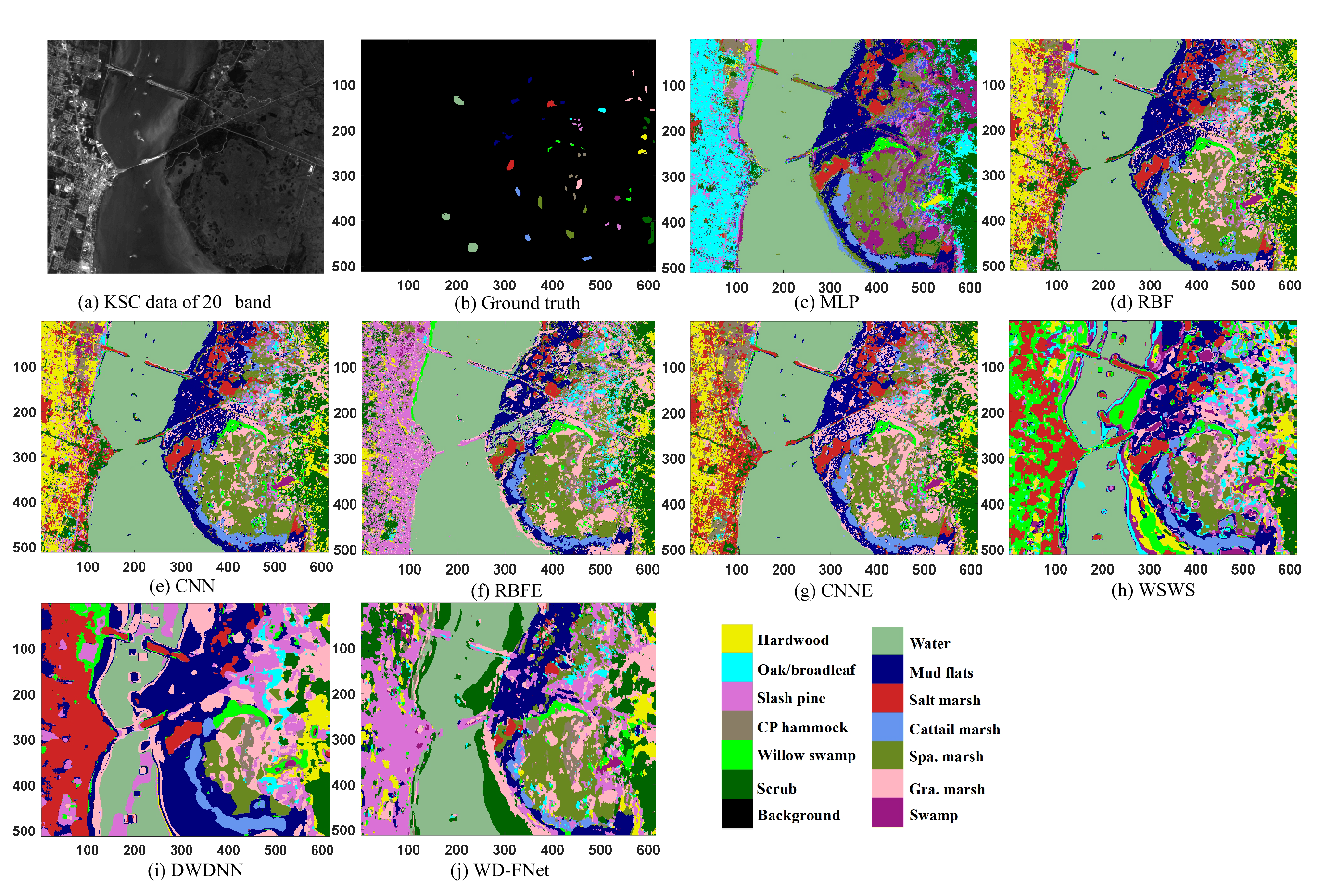
| Class NO. | MLP | RBF | CNN | RBFE | CNNE | WSWS | DWDNN | WD-FNet |
|---|---|---|---|---|---|---|---|---|
| 1 | 99.78 | 98.47 | 97.37 | 96.94 | 97.81 | 100.00 | 100.00 | 100.00 |
| 2 | 99.31 | 88.28 | 94.48 | 92.41 | 94.48 | 100.00 | 100.00 | 100.00 |
| 3 | 92.86 | 96.75 | 95.45 | 96.10 | 98.70 | 99.35 | 100.00 | 100.00 |
| 4 | 79.61 | 64.74 | 76.97 | 71.71 | 70.39 | 100.00 | 98.68 | 99.34 |
| 5 | 87.63 | 90.72 | 72.16 | 92.78 | 69.07 | 96.91 | 100.00 | 100.00 |
| 6 | 99.27 | 88.32 | 83.21 | 83.21 | 86.13 | 100.00 | 100.00 | 100.00 |
| 7 | 100.00 | 96.83 | 100.00 | 95.24 | 90.48 | 100.00 | 100.00 | 100.00 |
| 8 | 100.00 | 98.07 | 96.53 | 94.98 | 99.61 | 100.00 | 100.00 | 100.00 |
| 9 | 100.00 | 100.00 | 100.00 | 100.00 | 100.00 | 100.00 | 100.00 | 100.00 |
| 10 | 99.59 | 99.59 | 100.00 | 97.93 | 100.00 | 100.00 | 100.00 | 100.00 |
| 11 | 98.41 | 90.84 | 100.00 | 95.62 | 100.00 | 100.00 | 100.00 | 100.00 |
| 12 | 99.34 | 98.01 | 96.01 | 98.67 | 98.34 | 100.00 | 100.00 | 100.00 |
| 13 | 100.00 | 100.00 | 100.00 | 100.00 | 100.00 | 100.00 | 100.00 | 100.00 |
| OA | 97.95 | 95.36 | 95.75 | 95.52 | 95.97 | 99.87 | 99.94 | 99.97 |
| AA | 96.60 | 93.10 | 93.25 | 93.51 | 92.69 | 99.71 | 99.90 | 99.95 |
| Kappa | 97.72 | 94.85 | 95.28 | 95.03 | 95.52 | 99.86 | 99.93 | 99.96 |
| Class NO. | MLP | CNN | 2-D CNN | 3-D CNN | SMSB | WSWS | DWDNN | WD-FNet |
|---|---|---|---|---|---|---|---|---|
| 1 | 100.00 | 98.51 | 100.00 | 98.41 | 99.78 | 100.00 | 100.00 | 100.00 |
| 2 | 100.00 | 99.82 | 99.96 | 100.00 | 99.97 | 99.87 | 99.91 | 100.00 |
| 3 | 99.41 | 99.66 | 99.63 | 99.23 | 99.94 | 98.82 | 99.24 | 100.00 |
| 4 | 99.52 | 98.68 | 99.28 | 99.90 | 99.28 | 97.73 | 98.80 | 100.00 |
| 5 | 97.70 | 99.38 | 99.20 | 99.43 | 99.54 | 99.38 | 99.88 | 99.88 |
| 6 | 100.00 | 99.96 | 100.00 | 99.55 | 99.97 | 99.96 | 100.00 | 100.00 |
| 7 | 0.00 | 99.95 | 100.00 | 99.72 | 99.88 | 99.91 | 99.95 | 100.00 |
| 8 | 90.64 | 74.24 | 93.62 | 89.75 | 98.87 | 99.72 | 99.81 | 99.91 |
| 9 | 100.00 | 100.00 | 100.00 | 99.81 | 99.91 | 99.76 | 99.70 | 99.92 |
| 10 | 99.08 | 93.44 | 98.82 | 98.36 | 98.85 | 99.64 | 99.95 | 100.00 |
| 11 | 99.53 | 96.72 | 99.73 | 98.12 | 99.79 | 100.00 | 99.84 | 100.00 |
| 12 | 100.00 | 99.74 | 100.00 | 98.96 | 99.94 | 99.91 | 99.74 | 100.00 |
| 13 | 99.64 | 98.91 | 100.00 | 98.93 | 99.03 | 99.82 | 99.82 | 100.00 |
| 14 | 99.84 | 100.00 | 99.86 | 98.60 | 98.86 | 100.00 | 99.69 | 100.00 |
| 15 | 85.53 | 88.65 | 91.52 | 79.31 | 97.63 | 99.52 | 99.56 | 100.00 |
| 16 | 99.91 | 98.53 | 99.92 | 94.51 | 99.92 | 100.00 | 99.72 | 99.45 |
| OA | 89.27 | 92.42 | 97.39 | 93.95 | 99.26 | 99.67 | 99.76 | 99.95 |
| AA | 91.92 | 96.64 | 98.85 | 97.02 | 99.45 | 99.63 | 99.73 | 99.95 |
| Kappa | 88.20 | 91.69 | 97.07 | 93.31 | 99.17 | 99.63 | 99.73 | 99.94 |
| Neighborhood Sizes | Pavia Univ. /(%) | KSC/(%) | Salinas/(%) | ||||||
|---|---|---|---|---|---|---|---|---|---|
| OA | AA | Kappa | OA | AA | Kappa | OA | AA | Kappa | |
| 96.68 | 93.96 | 95.63 | 94.63 | 92.18 | 94.04 | 96.46 | 98.33 | 96.08 | |
| 98.05 | 96.16 | 97.38 | 96.87 | 95.16 | 96.52 | 97.56 | 98.81 | 97.30 | |
| 98.70 | 97.40 | 98.05 | 98.18 | 96.98 | 97.97 | 98.43 | 99.33 | 98.26 | |
| 99.22 | 98.52 | 98.97 | 99.04 | 98.06 | 98.93 | 98.98 | 99.46 | 98.87 | |
| 99.35 | 98.71 | 99.13 | 99.07 | 98.10 | 98.97 | 99.49 | 99.76 | 99.43 | |
| 99.59 | 99.20 | 99.46 | 99.30 | 98.87 | 99.22 | 99.73 | 99.79 | 99.70 | |
| 99.77 | 99.55 | 99.69 | 99.49 | 99.40 | 99.43 | 99.89 | 99.95 | 99.88 | |
| 99.51 | 99.10 | 99.35 | 99.97 | 99.95 | 99.96 | 99.88 | 99.93 | 99.87 | |
| 99.44 | 98.64 | 99.26 | 99.81 | 99.66 | 99.79 | 99.95 | 99.95 | 99.94 | |
| 99.41 | 98.57 | 99.22 | 99.39 | 99.27 | 99.32 | 99.95 | 99.98 | 99.95 | |
Publisher’s Note: MDPI stays neutral with regard to jurisdictional claims in published maps and institutional affiliations. |
© 2022 by the authors. Licensee MDPI, Basel, Switzerland. This article is an open access article distributed under the terms and conditions of the Creative Commons Attribution (CC BY) license (https://creativecommons.org/licenses/by/4.0/).
Share and Cite
Xi, J.; Ersoy, O.K.; Cong, M.; Zhao, C.; Qu, W.; Wu, T. Wide and Deep Fourier Neural Network for Hyperspectral Remote Sensing Image Classification. Remote Sens. 2022, 14, 2931. https://doi.org/10.3390/rs14122931
Xi J, Ersoy OK, Cong M, Zhao C, Qu W, Wu T. Wide and Deep Fourier Neural Network for Hyperspectral Remote Sensing Image Classification. Remote Sensing. 2022; 14(12):2931. https://doi.org/10.3390/rs14122931
Chicago/Turabian StyleXi, Jiangbo, Okan K. Ersoy, Ming Cong, Chaoying Zhao, Wei Qu, and Tianjun Wu. 2022. "Wide and Deep Fourier Neural Network for Hyperspectral Remote Sensing Image Classification" Remote Sensing 14, no. 12: 2931. https://doi.org/10.3390/rs14122931