Ocean–Atmosphere Variability in the Northwest Atlantic Ocean during Active Marine Heatwave Years

Abstract

The Northwest (NW) Atlantic has experienced extreme ecological impacts from Marine Heatwaves (MHWs) within the past decade. This paper focuses on four MHW active years (2012, 2016, 2017, and 2020) and the relationship between Sea Surface Temperature anomalies (SSTA), Sea Surface Salinity anomalies (SSSA), North Atlantic Oscillation (NAO), Geopotential Height anomalies (ZA), and anomalous Jet Stream positions (JSPA). Multichannel singular spectrum analysis (MSSA) reveals the strongest temporal covariances between SSSA and SSTA, and JSPA and SSTA for all years, particularly for 2020 (SSSA–SSTA: 50%, JSPA–SSTA: 51%) indicating that this active MHW year was more atmospherically driven, followed by 2012, which had the second highest temporal covariances (SSSA–SSTA: 47%, JSPA–SSTA: 50%) between these parameters. Spatial correlations for SSSA and SSTA between NAO during MHW active years disrupt the long–term (2010–2020) positive relationship in the NW Atlantic. SSSA and JSPA, and SSSA and SSTA were strongly correlated across the NW Atlantic; 2012 SSSA–JSPA correlations were strong and positive between 56–62°W, and 2016, 2017, and 2020 SSSA–JSPA correlations were mostly strong and negative, with strong positive correlations present near the coastline (70–66°W) or off the NW Atlantic shelf (52–48°W). SSSA–SSTA showed the opposite correlations of similar spatial distributions of SSSA–JSPA for all MHW active years. This indicates strong relationships between JSPA, SSSA, and SSTA during MHWs. Understanding the temporal and spatial interplay between these parameters will aid in better monitoring and prediction of MHWs.

1. Introduction

Marine Heatwaves (MHWs) are extreme warming events that have been increasing in duration, frequency, and intensity, posing adverse effects to local marine ecosystems [1,2]. They are defined by an event of Sea Surface Temperature anomalies (SSTA) above the 90th percentile of climatological seasonal SST variations for at least 5 continuous days [3]. MHWs are globally occurring events that have a variety of drivers [4,5,6] with notable events in the west coast of Australia (2010/2011) [7], Tasman Sea (2015/2016) [8], the Northeast Pacific (2015, 2016) [9], the Northwest Pacific (2021) [10], the Red Sea (2010, 2017, 2018, 2019) [11], and the Mediterranean Sea (2020) [12,13]. The Northwest (NW) Atlantic experiences frequent MHWs, and these events have been caused by oscillations of the Jet Stream (JS) and maintained by its pertinent northward shift [4,14]. MHWs are difficult to predict due to their variety of spatio–temporal scales and the nonlinear physical properties associated with MHW formation [15]. Throughout the past decade, there have been four anomalously MHW active years (2012, 2016, 2017, and 2020) in the NW Atlantic. The 2012 MHW formation was induced by an anomalously northward JS through the autumn and winter of 2011–2012, with strong JS variability into the spring and summer, building the MHW in the Gulf of Maine (GOM) and allowing the duration of this event to extend throughout the year with an increased impact on the local ecosystem, as seen in the declined recruitment of GOM cod and yellowtail flounder, and the economic failings of the lobster fishery [2,14]. The 2016 MHW was induced by the same forcings as 2012 in late winter through spring 2016, but ocean advection maintained high SSTAs through the summer months until anomalous JS positions forced yet another MHW in autumn of 2016 [16]. The 2017 MHW was induced by a Warm Core Ring intruding its water mass on the shelf along the Middle Atlantic Bight (MAB) in early 2017 that additional air–sea fluxes pushed the MHW in the NW Atlantic [17]. While there have not yet been any peer–reviewed journal articles on MHWs in the NW Atlantic for 2020, global temperatures matched the 2016 record [18], and upper ocean temperatures hit a new record high with the NW Atlantic having one of the highest Ocean Heat Content anomalies in the upper 2000 m of the water column [19]. This indicates that 2020 as an important year to monitor the formation of MHWs and a new aspect of this study. While 2012 is considered to be the most atmospherically forced MHW of these four years [20], understanding how atmospheric parameters, such as the JS, interact with the ocean’s surface will be key to monitoring their formation and duration. JS variability patterns are described using the variability of the North Atlantic Oscillation (NAO), where a positive phase often indicates a poleward shift [21]. Petrie (2007) [22] states that a positive wintertime NAO leads to warmer waters in the NW Atlantic, a process that aided in the 2012 and 2016 MHWs.

Another facet of surface MHWs not well studied are the changes in salinity. The NW Atlantic is influenced by its western boundary current, the Gulf Stream, which brings additional warm waters with higher salinity onto the continental shelf and can reinforce atmospherically–driven MHWs [16,17,23]. Salinity has been used in previous studies in the NW Atlantic to understand the formation of MHWs through ocean advection or changes in heat flux [17,20,24,25]. Since salinity has less variability than other oceanic parameters, Sea Surface Salinity anomalies (SSSAs) can be used for monitoring the formation of MHW events in this study as advective processes can be seen using SSS [26]. Salinity is also affected by atmospheric processes, specifically evaporation and precipitation due to convection modulated by changes in heat flux. These processes impact salinity differently, which is why new insight is needed on the ability of SSS to track the formation of MHWs to broaden the knowledge of monitoring MHWs as they intensify and respond to multiple processes. Analyzing SSS variability with atmospheric parameters is a new aspect of this study for MHW active years. ESA’s Soil Moisture Ocean Salinity (SMOS) SSS covered the desired temporal and spatial scales for these MHW active years in the NW Atlantic, providing the ideal salinity coverage to compare with the atmospheric parameters used in this study.

The main objective of this work is to better understand the dynamical relationship between atmospheric and oceanic parameters, JS latitude position, geopotential height (Z), NAO, SST, and SSS to better monitor the development of MHWs in the NW Atlantic. Comparing parameters present in the formation of the four MHW active years will also provide understanding of their role in the duration of each event. The NW Atlantic for this study will be focused on the Center Shelf, Center Slope, North Shelf, and North Slope (40–48°N, 48–70°W) as outlined in Perez et al. (2021) [16]. This region has been severely impacted by the MHWs and is among the fastest warming regions in the ocean [23]. Understanding how NAO and atmospheric parameters encourage the formation of MHWs is important for the monitoring of these events and for more accurately deploying warnings and initiating relief measures to affected marine ecosystems. An overview of the atmospheric parameters, spatial SSTAs, spatial SSS, and the NAO index used in this work, and the description of our methodology of our analysis follows in Section 2. Results are presented in Section 3 and discussed in Section 4. We conclude this work in Section 5.

2. Materials and Methods

To identify and quantify the location and timing of MHWs, the daily Optimum Interpolation Sea Surface Temperature (OISST) was used for our SST analysis. SST analyses used in this study were provided by NOAA’s National Center for Environmental Information at a global resolution of 0.25°. SSTAs are calculated with daily OISST minus a 30–year climatological mean at the same 0.25° spatial resolution. Hobday et al. (2016) [3] recommends that SST data used in MHW studies have 30–year climatological baselines. OISST has been reliably used to identify and study MHWs [1,3,4,6,13,16,24,27,28].

Debiased SMOS SSS Level 3 version 7 maps generated by LOCEAN/ACRI–ST Ocean Salinity Center of Expertise for CATDS provided the salinity data from January 2010 to November 2021 to calculate the SSSAs for this study. The V7 maps are provided every 4 days, and the debiased SSS are temporally averaged using a slipping Gaussian kernel with a full width at half maximum of 9 days for the 9–day product. Maps are at a spatial resolution of 25 km with an applied mean over neighbor pixels at less than 30 km for the purpose of producing debiased SSS maps. To account for the differences in temporal and spatial resolution between the debiased SSS and OISST, the SMOS SSS maps were re–gridded to OISST resolution.

All atmospheric parameters used in this work (zonal and meridional winds at 300 hPa, geopotential height at 300 hPa, and monthly averaged surface thermal radiation) are courtesy of the European Centre of Medium–Range Weather Forecasts (ECMWF). We use their newest product (ERA5), ECMWF’s fifth generation reanalysis, which improves upon the previous ERA–Interim dataset with better temporal and spatial resolution, more available parameters, and a variety of new instruments and reprocessed datasets. Like the OISST, we use 0.25° daily files and the 300 hPa pressure level to observe the upper atmosphere including the JS. We are confident in this dataset’s capability for the study of MHWs, as shown in Perez et al. (2021) [16] and Schlegel et al. (2021) [24].

The National Weather Service’s Climate Prediction Center NAO Index was used in this work to determine the state of the NAO. This daily index is computed by applying Rotated Principal Component Analysis to 500 mb heights north of 20°N with respect to the 1950–2000 climatological mean, and anomalies are with respect to this mean.

General Bathymetric Chart of the Oceans provided the global terrain model, GEBCO_2021 Grid, used to interpret spatial correlation maps and dynamics within the NW Atlantic [29]. GEBCO_2021 provides elevation data, in meters, on a 15 arc–second interval grid. A Type Identifier (TID) grid accompanies the GEBCO Grid, where corresponding grid cells indicate the source data for that cell with a variety of direct and indirect measurements.

An MHW is a prolonged discrete anomalously warm water event. Hobday et al. (2016) [3] were the first to define an MHW as an event with temperatures that exceed the 90th percentile of an established climatology (recommending a climatology based on at least 30 years) for five or more days. This definition has been adopted by the literature [2,4,16,17,28,30] on MHWs. Using literature that cited Hobday et al. (2016) [3] to define multiple or long–lasting MHW events in the NW Atlantic, we identified four MHW active years, 2012, 2016, and 2017. The 2012 MHW is considered the most extreme year, with SSTAs in the GOM with over 100 days above the 90th percentile; the 2016 MHWs lasted over 4 months over 2 events with conditions consistently above the 90th percentile from January to mid–April and September to late November [2,16,24]. In 2017, a similar pattern of split MHWs occurred with February through April having strong positive SSTAs [17]. MHWs from 2020 are not well studied in the NW Atlantic, but as they have record ocean temperatures and ocean heat content for the NW Atlantic in a region with frequent MHWs, it is a year important to include in this study [4,5,6,18,19]. The region selected for the NW Atlantic (40–48°N, 48–70°W) focusing on the Center Shelf, Center Slope, North Shelf, and North Slope are as outlined in Perez et al. (2021) [16].

To determine the location of the Northern Hemisphere Jet Stream (JS) to the GOM, we use the same methodology as Belmecheri et al. (2017) [31]. The JS in the northern hemisphere is often fragmented over land but becomes a single stream over the North Atlantic, therefore making a single–stream index more accurate [31,32,33]. The Jet Stream Index (JSI) identifies the latitude of the strongest 300 hPa wind speed at each available longitude [34]. To remove the seasonality of the JS, the JSI was calculated daily for each longitude from 1981–2020 and averaged to calculate the daily climatological mean JS position. The Jet Stream Position Anomaly (JSPA) is with respect to this position. The seasonality of daily geopotential height at 300 hPa, monthly surface thermal radiation (STR), and SST was removed when the respected climatological mean from 1981–2020 was subtracted from the data, providing the geopotential height anomaly (ZA), STR anomaly (STRA), and SSTA. SSS anomalies (SSSAs) were calculated from the available SMOS data, 2010–2021.

Multichannel singular spectrum analysis (MSSA), which is an ideal method for analyzing temporal and spatial correlations between different time series related to climate variability or ocean–atmosphere dynamics [35,36], was applied to the time series of each parameter averaged in the NW Atlantic focused box (40–48°N, 48–70°W). The bounds of this box were determined to include the Center and North Shelf and Slope around and outside biodiverse areas, such as the GOM and the Gulf of St. Lawrence (GSL) [16]. More detailed steps of MSSA are included in Grusszczynka et al. (2019) [36], Groth and Ghil (2011) [37], and Zotov and Scheplova (2016) [38]. Two time series are combined in a trajectory matrix, where the corresponding eigenvectors and eigenvalues are produced by applying Singular Value Decomposition. With the known original structure of the matrix, the Principal Components (PCs) are reconstructed, where each PC mode decreases in amplitude, representing the time series variability [36]. With seasonality removed from each time series by using the calculated anomalies, the variance of the PCs will be reduced, but the first PC having a high variance indicates a strong correlation in the variability of each time series.

3. Results

Spatial comparison between daily SSTA, JS position, and the mean JS position calculated daily from 1981–2020, throughout the year for MHW active years 2012 (Figure 1), 2016 (Figure 2), 2017 (Figure 3), and 2020 (Figure 4) show the propagation of MHWs in each year. Seasonally averaging SSTAs and the position of the JS, during the formation and decline of MHWs, removes the noticeable features of these events as these parameters have a high temporal variance. To account for this, six dates for each year were chosen to show days prior to onset, early onset, close to peak, and declines in the MHW active years while also being seasonally comparable to other years. The dates were chosen in January, March, May, July, September, and October.

From the beginning of 2012 to March 2012, strong positive SSTA anomalies are spatially contained to the Center Slope and Center Shelf, specifically in the (40–48°N, 48–70°W) box which we focus on throughout this study (Figure 1a, average = 1.15 °C; Figure 1b, average = 1.13 °C). Figure 1c shows the peak of the MHW intensity within the GOM in late May (average = 1.95 °C), with the JS meandering above the climatological mean position above the GOM and GSL. Throughout the rest of the year (Figure 1d, average = 2.10 °C; Figure 1e, average = 2.01 °C; Figure 1f, average = 2.47 °C), the positive SSTAs extend throughout the entire NW Atlantic, as the MHW fully formed, coinciding with the climatological northward movement of the JS. While the JS position from summer through the end of 2012 is not north of the climatological mean, the anomalous position occurred during the formation of this MHW in the first half of the year [14], and the extension of the event away from the coastline.

The 2016 MHWs were much less intense than the 2012 events. SSTAs were stronger in the earlier parts of the year (Figure 2a, average = 0.65 °C; Figure 2b, average = 0.32 °C) and later months (Figure 2e, average = 0.75 °C; Figure 2f, average = 1.62 °C). Positive SSTAs were contained closer to the coastline and southward where the Gulf Stream likely plays a role, while negative SSTAs were north and to the east most noticeably seen in early spring (Figure 2b) and mid–summer (Figure 2d, average = 0.20 °C). Figure 2c is the only exception where strong negative SSTAs follow the coast in the shelf region (average = 0.15 °C). The JS does not meander as in 2012 (Figure 1) or have a noticeable change from the climatological mean position, except in summer (Figure 2d) where the JS splits above the mean position.

The 2017 MHWs were the coolest MHW active year in this study, with widespread average SSTAs not reaching above 1.5 °C (Figure 3). The boxed region had strong negative SSTAs either along the slope (Figure 3a, average = 1.04 °C; Figure 3b, average = 0.31 °C; Figure 3d, average = 0.65 °C; Figure 3f, average = 1.06 °C) or throughout the full region (Figure 3c, average = −0.13 °C; Figure 3e, average = −0.3167 °C). Pershing et al. (2018) [2] describes 2017 as a cool year prior to the Maine lobster season, which can be seen in spring and early summer (Figure 3b,c). The JS position in 2017 followed the climatological mean with any deviations generally being south as seen in Figure 3a,c,e. Gawarkiewicz et al. (2019) [17] credits the MHW formation as an advective MHW where the formation is less influenced by atmospheric processes.

The 2020 MHWs began in the summer and extended through the end of the year, similar to 2016 and 2017. Unlike those years, there was no presence of strong MHWs occurring in the beginning of the year (Figure 4). Strong negative SSTAs in the spring were pervasive in the NW Atlantic (Figure 4b, average = 0.14 °C; Figure 4c, average = −0.92 °C). Figure 4d (average = 1.08 °C) and Figure 4f (average = 1.95 °C) are the only shown dates with the GOM and the GSL having positive SSTAs, showing that these MHWs were more focused along the slope. As in Figure 3, the JS in 2020 stayed close to the mean JS position except for Figure 4d, where the JS meandered far north of the mean position with a shift north of around 10°N with the JS positioned at 58°N.

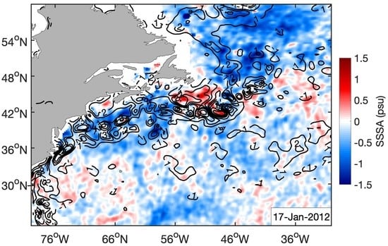
Spatial comparison between SSSA from SMOS, JS position, and the climatological JS position throughout the year for MHW active years 2012 (Figure 5), 2016 (Figure 6), 2017 (Figure 7), and 2020 (Figure 8) show the propagation of MHWs in each year with salinity. Figure 5, Figure 6, Figure 7 and Figure 8 display the same dates as Figure 1, Figure 2, Figure 3 and Figure 4 to gain an understanding of how SSSA and SSTA propagate differently during the same MHW, and how the position of the JS impacts these parameters.

Figure 5 shows persistent and strong negative SSSA anomalies throughout the NW Atlantic in 2012. This is likely from the shift in ocean circulation from changes in NAO and associated wind stress curl patterns which caused a freshening event to occur from 2012–2016 in the NW Atlantic [39], causing much of the average SSSAs to be negative. A positive SSSA maximum, varying between 1.07 and 1.93 psu, was persistent throughout 2012 within the NW Atlantic with a longitude between 56–50°W (Figure 5). In March, as the MHW began to form in the GOM, positive SSSAs were present along the coastline and south of the NW Atlantic box (Figure 5b, average = −0.1172 psu, max = 1.93 psu). May 2020 had the lowest SSSA maximum (1.07 psu) and average (−0.21 psu) (Figure 5c). During the summer, the NW Atlantic was the highest in salinity for 2020 (Figure 5d, average = 0.07 psu, max = 1.68 psu). Figure 5e (average = −0.12 psu, max = 1.42 psu) and 5f (average = −0.17 psu, max = 1.30 psu) showed higher salinity waters were maintained closer to the coastline and in the GOM and GSL.

In contrast to 2012, 2016 SSSAs were more positive throughout the year (Figure 6). Within the confines of the NW Atlantic box used in this study, positive SSSAs were more prevalent in the southeast edge of the box, away from the coastline and freshwater inflow. Figure 6a shows January to have a widespread positive SSSA with an average of 0.17 psu and a maximum of 1.99 psu. Figure 6b (average = −0.02 psu) shows the addition of freshwater moving along the coast from further north to the NW Atlantic, where the lower SSSAs remain along the North and Center Shelf, slowly dissipating through the duration of MHWs (Figure 6c, average = 0.16; Figure 6d, average = −0.02 psu; Figure 6e, average = 0.12 psu; Figure 6f, average = 0.14 psu). Preceding the increase in SSTAs in later months (Figure 2e,f), there was a strengthening of positive and negative SSSAs, with maximum SSSAs equaling 1.94, 1.91, and 2.05 psu, and minimum SSSAs equaling −1.27, −1.61, and −1.41 psu (Figure 6d–f).

The 2017 MHW SSSAs were similar to the 2016 MHW SSSAs. January had widespread positive SSSAs averaged to 0.24 psu (Figure 7a), with March receiving lower salinity water in the NW Atlantic averaging to −0.03 psu with minimum SSSAs equaling −1.56 psu (Figure 7b). The 2017 MHWs also experienced the strengthening of positive and negative SSSAs during the formation and lifespan of the MHW as in 2016. SSSAs were their strongest in summer through early autumn with the peaking of the MHW (Figure 7d, min = −2.26 psu, max = 1.99 psu; Figure 7e, min = −1.39 psu, max = 1.84 psu). SSSAs became less extreme in October (Figure 7f, min = −1.47 psu, max = 1.43 psu).

It was found that 2020 had more persistent and stronger SSSAs in the NW Atlantic than all other MHW years (Figure 8). Positive SSSAs were also persistent outside of the GSL and to the northeast of the boxed region (Figure 8). From the beginning of the year to late spring, a strong negative SSSA moved westward into the GOM and increased in size, with the center of this water body staying between −1.40 to −1.80 psu (Figure 8a–c). Figure 8b shows early spring having widespread positive SSSAs that averaged to 0.08 psu. Summer to the end of the year experienced similar patterns of strengthening SSSAs as the MHW developed and peaked in 2020 as the other MHW active years. Negative SSSAs were stronger in the NW Atlantic box in Figure 8d (min = −1.90 psu), Figure 8e (min = −1.78 psu), and Figure 8f (min = −1.24 psu). Positive SSSAs peaked in early autumn (Figure 8e) with maximum values of 1.96 psu, while surrounding months had maximum positive SSSAs below 1.71 psu (Figure 8d,f).

Figure 9 shows the spatial correlation coefficients between daily SSTA and NAO (Figure 9a,c,e,g,i), and SSSA and NAO (Figure 9b,d,f,h,j) for 2012 (Figure 9a,b), 2016 (Figure 9c,d), 2017(Figure 9e,f), 2020 (Figure 9g,h), and the time series of 2010–2020 (Figure 9i,j). NAO is known to influence SST in the North Atlantic and can increase the possibility of MHWs in other regions of the North Atlantic [28]. These yearly correlations between oceanic parameters and daily NAO compare the effects of NAO variability on each MHW active year. There was no widespread correlation with strong divides within the NW Atlantic boxed region for each MHW active year which reduced the average correlation value to near zero. This contrasts with the time series correlations (Figure 9i,j) which have mostly weak positive correlations in the NW Atlantic, and individual events have been smoothed out based on the length of the time series. In the boxed NW Atlantic region, SSTA and NAO positive correlation were present along the 1000 m shelf break in 2012 (Figure 9a, max = 0.6012) and 2016 (Figure 9c, max = 0.4161), while correlations in 2020 (Figure 9g, max = 0.3914) were contained near the GOM. The positive correlations in 2017 for SSTA and NAO were focused in the GOM and on the eastern end of the shelf contained in the box (Figure 9e, max = 0.4207). For SSSA and NAO in the boxed region, there were very scattered positive correlations, but south of the GSL, along the 1000m shelf break, there were consistently positive correlations (Figure 9b,d,f,h). In 2016 (Figure 9d) and 2017 (Figure 9f), there were more positive correlations along the coast and on the shelf region. Figure 9h also shows positive correlations for SSSA and NAO slope–ward of the 1000 m shelf break for the 2020 MHW year.

The time series (Figure 10) shows the temporal variance within the boxed region of the NW Atlantic of NAO, SSSA, SSTA, and the JS position anomaly (JSPA), calculated from the latitude of the daily wind magnitude maximum at 300 hPa between 23–60°N minus the climatological mean latitude, then averaged across 70–48°W. The JSPA is the most variable parameter and maintains a negatively anomalous position throughout each year with the minimum positions occurring during the periods of elevated SSTAs, which are indicated with light gray boxes (Figure 10). Figure 10a shows the 2012 time series where SSSA was very low for most of the year with peaks into positive anomalies occurring with and slightly prior to SSTA peaks in April and July to November. NAO also followed this pattern with positive peaks occurring with SSSA peaks (Figure 10a). In early 2012, while JSPA does not become positive, NAO peaks were preceded by peaks in JSPA, but this pattern stopped occurring after May, as the JS remained south of the climatological mean in the summer and autumn as seen in Figure 1d–f (Figure 10a). Figure 10b shows the 2016 time series. SSSA was more variable and had mostly positive anomalies for 2016. Mid–January to mid–March there was a small MHW where SSTA, SSSA, and NAO had a high plateau before dropping; in early January, JSPA was positive before this event occurred (Figure 10b). Other peaks of high SSTA and SSSA occurred in July to August and November to December, and NAO had a peak prior to these events (Figure 10b). These peaks were connected by constant SSTAs above 1 °C; this was where JSPA reached its maximum decline for 2016 (Figure 10b). Figure 10c shows the 2017 time series. The beginning of the year had high SSSAs which SSTAs were decreasing, becoming negative, and NAO slowly decreasing with oscillations through spring (Figure 10c). During this time, JSPA was oscillating just below zero (Figure 10c). Later in the year, July to August and November to December, peaks of NAO were followed by higher SSTAs and SSSA peaks (Figure 10c). Figure 10d shows the 2020 time series. JSPA from January through April experienced a positive peak monthly before rapidly moving south of the climatological mean for the rest of the year (Figure 10d). NAO appeared to follow the reverse of JSPA, with negative peaks while JSPA was positive (Figure 10d). Once JSPA steeply dropped in mid–May, SSTAs increased through the end of the year, while reaching a brief peak in August (Figure 10d). SSSA began close to zero and slowly increased from July to November with elevated SSTAs (Figure 10d). To focus on how SSTA and atmospheric parameters vary temporally, Figure 11 shows the time series of JSPA, SSTA, geopotential height anomalies (ZA) at 300 hPa, and Surface Thermal Radiation anomalies (STRA). STRA loosely followed the variability of JSPA except in September to October in 2017 (Figure 11c) and May to July in 2020 (Figure 11d). STRA increasing or positive indicates the JS was not removing heat from the ocean, such as in November 2012 (Figure 11a), March, June, and November 2016 (Figure 11b), May and October 2017 (Figure 11c), and July 2020 (Figure 11d). ZA oscillated around zero without a noticeable increase or decrease, but did experience larger positive peaks during elevated SSTAs, indicated by the light gray boxes (Figure 11).

Time lag composites show the spatial cross–correlations from 48–70°W within the NW Atlantic. Figure 12 shows the time lag composites between atmospheric parameters and SSTA. Cross–correlations between JSPA and SSTA (Figure 12a–d) were extremely negative, except east of 50°W in 2016 (Figure 12b) and 2017 (Figure 12c), where the North shelf reached its longitudinal extent. The most negative correlations were near zero lag days further out on the NW Atlantic slope, except for 2016 which had a lag of 25 days (Figure 12b), and 2017 which had a lead of 25 days (Figure 12c). Cross–correlations between JSPA and ZA (Figure 12e–h) were mostly negative with no lag or lead, and small positive correlations of JSPA–ZA led close to 50 days near the coast for 2012 (Figure 12e), 2016 (Figure 12f), 2017 (Figure 12g), but lagging 50 days in 2020 (Figure 12h). The strongest correlation between JSPA–ZA for 2016 was east of every other year, with its position around 64°W (Figure 12f). Cross–correlations between SSTA and ZA (Figure 12i–l) were mostly positive with no lag or lead except for 2016 with a lead of 25 days (Figure 12j); 2012 (Figure 12m) and 2016 (Figure 12n) had almost all positive correlations between NAO–JSPA, while 2020 (Figure 12p) was mostly negative. Figure 12o shows 2017 NAO–JSPA correlations with a slight positive lag near the coast, and negative correlations further down the shelf. The maximum correlations between NAO–JSPA had a lag of 10 days for 2012 and 2017 (Figure 12m,o), a lead of 10 days for 2016 (Figure 12n), and a lead of 50 days in 2020 (Figure 12p). Correlations for NAO–SSTA for 2012 (Figure 12q) were the opposite of NAO–JSPA, or all negative with a negative correlation lag of 25 days; 2016 (Figure 12r), 2017 (Figure 12s), and 2020 (Figure 12t) had mostly positive correlations between NAO and SSTA, with the strongest positive correlations having NAO lead for 2016 by 0 days, for 2017 by 10 days, and for 2020 by 25 days.

Figure 13 shows time composites between SSSA and the other parameters. From JSPA and SSTA having such a strong negative correlation, the strong correlations SSSA had with these parameters were near inverses of each other; 2012 SSSA–JSPA (Figure 13a) were very positive between 56–62°W with SSSA–SSTA (Figure 13e) having strong negative correlations in the region; 2016 SSSA–JSPA (Figure 13b) were mostly negative, while SSSA–SSTA (Figure 13f) were mostly positive correlations, and 2017 SSSA–JSPA (Figure 13c) were very positive between 66–70°W, 58–62°W, and at 52°W, with SSSA–SSTA (Figure 13g) having noticeable negative correlations near 70°W and east of 52°W. The 2020 SSSA–JSPA (Figure 13d) had strong positives closer to 70°W or along the coast and in the GOM, and strong negatives around 52°W or near the end of the North shelf, while SSSA–SSTA (Figure 13h) had strong negatives closer to 70°W and strong positives around 52°W. Correlations for SSSA–NAO were mostly positive with 2016 (Figure 13j), 2017 (Figure 13k), and 2020 (Figure 13l) having strong lags of 80 days (2016), 25 days (2017), and 10 days (2020). The 2012 correlations of SSSA–NAO (Figure 13i) followed the same distribution as Figure 13a, with weaker values and with a positively correlated lead of almost 100 days. The 2012 correlations of SSSA–ZA (Figure 13m) were not strong but had a slight positive correlation lead of 25 days near 50°W, and 2016 (Figure 13n) and 2017 (Figure 13o) had very weak positive lead correlations of 25 and 50 days. The 2020 correlations of SSSA–ZA (Figure 12p) loosely followed the distribution of Figure 13l with a positive correlation of 0 days.

Using the variance of PCs calculated in MSSA, the temporal relationship between the parameters, JSPA, SSSA, SSTA, and NAO, can be compared across years (Figure 14). The first PC should have the most variance, as it was reconstructed to model the most oscillations between the parameters. The higher the variance of this first PC, the stronger the temporal covariance pattern will be [36]. Figure 14 shows pairs of parameters JSPA–SSSA (Figure 14a–d), JSPA–SSTA (Figure 14e–h), SSSA–NAO (Figure 14i–l), SSSA–SSTA (Figure 14m–p), and SSTA–NAO (Figure 14q–t) for the first 5 PCs’ mode. SSSA–SSTA (Figure 14m–p) and JSPA–SSTA (Figure 14e–h) were the parameter pairs that had the highest temporal covariances, with 2020 (Figure 14h,p) as the year with the strongest covariances. Variance of the first PC for SSSA–SSTA was 47% for 2012 (Figure 14m), 34% for 2016 (Figure 14n), 41% for 2017 (Figure 14o), and 50% for 2020 (Figure 14p). Variance of the first PC for JSPA–SSTA was 50% for 2012 (Figure 14e), 35% for 2016 (Figure 14f), 40% for 2017 (Figure 14g), and 51% for 2020 (Figure 14h). SSTA–NAO (Figure 14q–t) followed with 2012 (Figure 14q) being the year with the strongest covariances. Variance of the first PC for SSTA–NAO was 41% for 2012 (Figure 14q), 30% for 2016 (Figure 14r), 32% for 2017 (Figure 14s), and 36% for 2020 (Figure 14t); 2017 (Figure 14c) was the year with highest temporal covariances of JSPA–SSSA (Figure 14a–d). Variance of the first PC for JSPA–SSSA was 32% for 2012 (Figure 14a), 20% for 2016 (Figure 14b), 39% for 2017 (Figure 14c), and 34% for 2020 (Figure 14d). The parameter pair with the lowest covariance was SSSA–NAO (Figure 14i–l). Variance of the first PC for SSSA–NAO was 38% for 2012 (Figure 14i), 18% for 2016 (Figure 14j), 22% for 2017 (Figure 14k), and 24% for 2020 (Figure 14l). For every parameter pair, 2016 had the least temporal covariance indicating that this MHW active year had other drivers that were likely oceanic–related, creating these MHWs. For SSSA and SSTA paired with NAO, 2012 had the highest covariance compared to the other years, indicating that NAO variability played a role in the intense MHW formation that occurred.

4. Discussion

The NW Atlantic has experienced four MHW active years within the past decade. Individual studies have identified 2012, 2016, and 2017 to be characterized by longer duration MHW events with severe quantifiable impacts on the ecosystem and fisheries. Global temperature and ocean heat content records identified 2020 as one of the warmest years in the NW Atlantic, experiencing conditions experienced in the other MHW active years. To compare the air–sea interactions of these four years, we used oceanic and atmospheric parameters (SSTA, SSSA, JSPA, ZA) and the NAO index. Using spatial maps of SSTA and SSSA, we were able to observe the formation of long duration MHWs in the NW Atlantic for the identified MHW active years with reference to the position of JS and its climatological position (Figure 1, Figure 2, Figure 3, Figure 4, Figure 5, Figure 6, Figure 7 and Figure 8). Time series also presented observations of MHW parameters with NAO (Figure 10) and atmospheric parameters with SSTA (Figure 11) throughout the active MHW years. MHW events in 2012 began in the GOM from April to May (averaged maximum = 1.75 °C) and formed a large event spread into the NW Atlantic from July to November (averaged maximum = 2.50 °C) (Figure 1 and Figure 10a). This year also experienced a prolonged northward position in the first half of the year which was not present during the other MHW active years [14]. Salinity for the 2012 MHW active year was negative for most of the NW Atlantic due to circulation shifts from NAO [39], but experienced SSSAs up to 1.68 psu (Figure 5d). The events in 2016 occurred from January to March (averaged maximum = 1.0 °C), July to August (averaged maximum = 1.90 °C), and November to December (averaged maximum = 2.0 °C) (Figure 2 and Figure 10b). SSSA had an average maximum of 0.25 psu for each MHW event in 2016 (Figure 10b). The events in 2017 occurred from July to August (averaged maximum = 1.0 °C) and November to December (averaged maximum = 1.0 °C) (Figure 3 and Figure 10c). The formation of MHW in 2017 in the Middle Atlantic Bight was attributed to a Warm Core Ring [17], which heavily influenced SSSAs in this region in the beginning half of the year but did not exceed 0.25 psu during the identified MHW months (Figure 10c). The events in 2020 occurred mid–June to October (averaged maximum = 1.95 °C) (Figure 4 and Figure 10d). SSSAs in 2020 stayed negative near the coastline while positive SSSAs increased in the east side of the NW Atlantic with an average maximum of 0.20 psu, and peak maximums reaching 1.96 psu (Figure 8e and Figure 10d).

To understand the dynamical relationship between these parameters during MHW years, we used spatial correlations, lag–lead correlations, and MSSA PCs’ variance for combined time series covariance. Figure 9 shows how during MHWs, NAO variability had an influence over SSTA and SSSA. In a long time series (2010–2020) (Figure 9i,j) these correlations had weak correlation coefficients but experienced a slight positive relationship in the NW Atlantic. During the MW active years, there was an increase in correlations and a disruption of their distribution. While major increases did not occur within the focused region, NAO increased positively with SSTA in the North Atlantic and west along the coast for SSSA. Figure 12 and Figure 13 show lead–lag days across the NW Atlantic for each pairing of parameters. Figure 14 shows PCs from MSSA and each combined time series covariances. As JS position is a previously known driver of MHWs in the NW Atlantic, strong relationships between JSPA and SSTA were expected to be seen (Figure 12a–d) [14]. The correlations between JSPA and SSTAs being strong negatives in Figure 12 were likely from the preconditioning that the JS position caused for the MHW, which occurred outside the lag–lead time relevant to the year, and the climatological position of the JS being very variable and seasonal, where the daily position anomaly became negative frequently [14,15]. Salinity and ocean temperatures experienced a similar relationship when MHWs form as shown in SSSA and SSTA (Figure 13a–h). Due to JSPA and SSTA’s strong negative relationship, the relationship between SSSA–JSPA and SSSA–SSTA is reversed (Figure 13a–h). Covariances of these 3 parameters were the 3 highest overall values, JSPA–SSTA, SSSA–SSTA, and JSPA–SSSA (Figure 14).

The 2012 MHW active year had a unique relationship with NAO, likely related to the shift occurring from 2012–2016 [39], as Figure 12m,q show all positive or negative correlations between JSPA and SSTA, respectively. This is further shown in the PCs’ covariance, where 2012 had the highest value compared to the other MHW years for SSSA–NAO and SSTA–NAO (Figure 14i,q). This shows the 2012 MHW was influenced by NAO variability along with JS variability as found in Chen et al. (2014) [14].

In 2020, the highest covariance of both JSPA–SSTA and SSSA–SSTA (51%, 50%) was observed, followed by 2012 (50%, 47%). The 2012 event was considered to be a MHW that was predominantly forced by atmospheric processes [14], indicating that the 2020 MHW is likely predominantly driven atmospherically. While 2020 was not as strongly influenced by NAO as 2012 was, the spatial correlations (Figure 9g,h) show a similar distribution where positive correlations increased along the shelf break.

In 2016 and 2017, more advectively formed MHWs [16,17] were observed where atmospheric forcing possibly aided in continuing their duration. While outside of the focus area, there were wider–spread positive correlations for both SSTA–NAO and SSSA–NAO in 2016 and 2017 (Figure 9c–f). Within the NW Atlantic, there were positive correlations along the shelf break, and between the shelf break and the coast (Figure 9c–f). This relationship was likely due to NAO influencing Warm Core Rings and MHW events occurring as these eddies crossed the shelf break. Figure 12b,c differed from Figure 12a,d by having strong positive correlations east of 50°W. This shift in correlation was likely from 2016 and 2017 being more advective, and the MHWs’ influence on SSTA occurring closer to the coast. The highest value of covariance between JSPA and SSSA was in 2017 (39%), indicating the advective MHW with its changes in salinity was influenced and intensified in the NW Atlantic by the JS. Finally, 2016 had the lowest covariance values for each paired parameter indicating that this MHW had predominantly oceanic forcings.

5. Conclusions

As MHWs continue to increase in frequency and intensity, understanding patterns of their formation is key to future prediction and monitoring of these events. Using atmospheric and oceanic parameters, the spatial and lead–lag correlations, and temporal covariance, we observed the variability occurring in the MWH active years 2012, 2016, 2017, and 2020 in the NW Atlantic. Spatial maps displayed the changing and propagation of the MHW active years in SSTA and SSSA, as the JS shifted position throughout the year. Each year experienced unique formations, but as positive SSTAs strengthened and became widespread, SSSAs became more extreme within the NW Atlantic. SSTA and NAO, and SSSA and NAO spatial correlations were not widespread with strong correlations located in small regions along the NW Atlantic shelf or slope. These small regions shown in the spatial correlations are essential locations where NAO affects MHW temperatures and salinity.

Due to JS position being a major driver in the NW Atlantic, and SSTA and SSSA related to characteristics of MHWs, lead–lag correlations were very strong between JSPA–SSTA and SSSA–SSTA. JSPA–SSTA and SSSA–SSTA also had the strongest temporal covariance as seen in the variance of PCs from MSSA. The highest covariance for JSPA–SSTA and SSSA–SSTA was observed in 2020 indicating that this MHW active year had the most forcings being atmospheric–related, much like 2012 which was known as a very atmospherically driven MHW [14]; 2012 had the second highest covariances for JSPA–SSTA and SSSA–SSTA, and the highest covariances for SSTA–NAO and SSSA–NAO, indicating 2012 was heavily influenced by the NAO index in addition to the JS. Finally, 2016 had the lowest covariance for each correlation pair, indicating that this MHW active year was not primarily atmospherically driven and instead was maintained by oceanic processes [16].

These parameters having strong correlations is not a new discovery; as temperature has been used to determine MHW events, JS are known drivers of MHWs in the NW Atlantic, and salinity is affected by other drivers of these MHWs [4,14,17,24]. The relationship of these parameters can be used to develop better monitoring of MHWs, as it is critical to understand the indicators and development of MHW activity. Future work quantifying the relationship of SSS and SST variability with atmospheric parameter variability, such as JS position, in the NW Atlantic is necessary to understand the formation of MHWs. More research on air–sea responses to other MHW drivers, such as ocean currents, is also needed in creating models designed to monitor and track MHWs. As accurate models can be expanded and applied to MHWs occurring globally, more research is important for being able to deploy relief measures for key ecosystems and fisheries.