Article

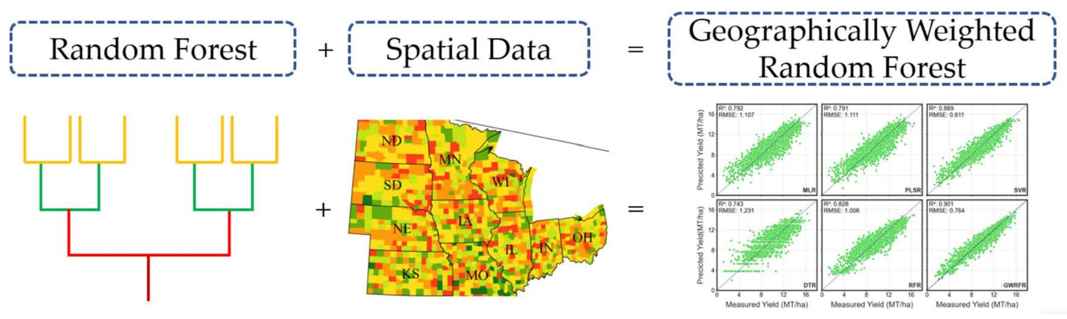
A Geographically Weighted Random Forest Approach to Predict Corn Yield in the US Corn Belt

by
Shahid Nawaz Khan
1,2,
Dapeng Li
1,* and
Maitiniyazi Maimaitijiang
1
1
Geospatial Sciences Center of Excellence, Department of Geography and Geospatial Sciences, South Dakota State University, Brookings, SD 57007, USA
2
Institute of Geographical Information Systems, National University of Sciences and Technology, Islamabad 44000, Pakistan
*
Author to whom correspondence should be addressed.
Remote Sens. 2022, 14(12), 2843; https://doi.org/10.3390/rs14122843
Submission received: 25 April 2022 / Revised: 3 June 2022 / Accepted: 9 June 2022 / Published: 14 June 2022

Abstract

:
Crop yield prediction before the harvest is crucial for food security, grain trade, and policy making. Previously, several machine learning methods have been applied to predict crop yield using different types of variables. In this study, we propose using the Geographically Weighted Random Forest Regression (GWRFR) approach to improve crop yield prediction at the county level in the US Corn Belt. We trained the GWRFR and five other popular machine learning algorithms (Multiple Linear Regression (MLR), Partial Least Square Regression (PLSR), Support Vector Regression (SVR), Decision Tree Regression (DTR), and Random Forest Regression (RFR)) with the following different sets of features: (1) full length features; (2) vegetation indices; (3) gross primary production (GPP); (4) climate data; and (5) soil data. We compared the results of the GWRFR with those of the other five models. The results show that the GWRFR with full length features (R2 = 0.90 and RMSE = 0.764 MT/ha) outperforms other machine learning algorithms. For individual categories of features such as GPP, vegetation indices, climate, and soil features, the GWRFR also outperforms other models. The Moran’s I value of the residuals generated by GWRFR is smaller than that of other models, which shows that GWRFR can better address the spatial non-stationarity issue. The proposed method in this article can also be potentially used to improve yield prediction for other types of crops in other regions.

Graphical Abstract

1. Introduction

Corn, as an important crop in the world, is mostly used for human food, ethanol production, and livestock feed [1]. The United States (US) is the largest corn producer and accounts for more than 36% of global corn production [2]. The majority of the corn produced by the US is from the Corn Belt, which consists of 12 Midwestern states where corn is usually grown in rotation with soybean [3]. The changing climate poses a threat to crop yield and the agricultural systems [4]. Additionally, the rapid growth of the global population also poses a challenge for global food security [5]. An accurate and timely yield estimation plays a significant role in agricultural economics and global food security because it can provide more information to different stakeholders such as farm managers, crop specialists, and governments and facilitate their decision making (e.g., importing/exporting grains, planting, irrigation, fertilizing, and harvesting) [6,7,8].
Crop yield prediction has attracted significant research attention [6,9,10,11,12,13,14,15,16,17,18,19,20,21,22,23,24,25,26,27,28,29] and can date back to 1964 [30]. There are two primary categories of crop yield models: physical models and statistical models [31]. Physical models use physiological conditions of crops and predict yield by incorporating the underlying processes such crop health, soil nutrients, and water availability [24]. Physical models usually provide better estimates of crop yield if the underlying crop conditions provided are accurate; however, these models are not widely used due to their complexity [32]. Physical models require fine-grained data, which limits the use of these models in large-scale applications, since it is difficult to compile the required detailed data for large study areas [31]. On the other hand, statistical models are widely used due to their simplicity and good performance [12,33,34]. Crop yield is affected by several factors such as genotype [17], weather [33], water management practices [35], soil moisture [14], and soil nutrients [36]. We can use these factors as the input to predict crop yield. In the early stages, soil-based parameters were mainly used to predict crop yield at the field level since other datasets were not available. With the development of data acquisition technologies, remote sensing and climate data have been widely used for crop yield prediction [28]. Recently, a significant amount of research has been conducted on crop yield prediction [11,15,19,20,25,31,34,37,38]. Different studies have used different datasets such climatic data [33], remote sensing data [21], and other biophysical data [23] to predict crop yield. Climatic variables such as temperature, precipitation, evapotranspiration, and vapor pressure deficit are related to crop growth as they can affect crop yield prediction [39].
Remote sensing data can provide information on both biotic and abiotic factors, such as temperature, precipitation, soil moisture, vegetation health, and water stress. One advantage of remote sensing data is their good availability. Early research [22] has demonstrated the effectiveness of remote sensing data in crop yield predictions. Since then, many studies [9,31,40] have been conducted on using satellite-derived information for crop monitoring and yield prediction. Remote sensing data can capture several crop characteristics such as crop health [41], diseases [42], and primary productivity [43]. The use of vegetation indices (VIs) derived from remote sensing data are more popular in crop yield prediction [44]. Compared with raw reflectance values, VIs are more sensitive to vegetation conditions and can better capture the changes in vegetation conditions such as crop growth, health, or stress [23]. VIs such as the normalized difference vegetation index (NDVI), enhanced vegetation index (EVI), soil-adjusted vegetation index (SAVI), green chlorophyll index (GCI), and normalized difference water index (NDWI) are generally used to characterize vegetation conditions and have recently been used to study crop yield [11,13,31,37]. NDVI and EVI have been calculated and used as independent variables in combination with several other variables such as climate and soil data to predict crop yield in different areas [11,31]. Another factor recently used for estimating crop yield is primary productivity [9], which can be defined as the amount of carbon taken by plants to create new biomass [45].
There are a variety of machine learning models that can be used to predict crop yield [16]. These input parameters of machine learning models include climate data (temperature, precipitation, evapotranspiration, and vapor pressure), soil conditions (soil organic carbon, soil moisture, and soil temperature), and management factors (planting pattern, sowing, and harvesting dates) [25]. Feng, Wang, Zhang and Du [11] developed a spatio-temporal neural network model that uses remote sensing, soil, and climate data to predict winter wheat yield. They also compared their results with those of other benchmark models such as support vector regression, and the results show that spatio-temporal models can improve winter wheat yield prediction by 2.61% in terms of mean absolute percentage error (MAPE). Ma, Zhang, Kang and Özdoğan [31] used Bayesian neural networks (BNN) to predict corn yield in the US Corn Belt and achieved a coefficient of determination (R2) of 0.77. The results of BNN were compared with those from other models, and their results show that BNN can reduce the overall error by 6 to 23%. Shahhosseini, Hu and Archontoulis [10] used machine learning ensembles to predict corn yield in three US states: Illinois, Iowa, and Indiana. A wide range of predictors were used to carry out this study, and their method can improve corn yield prediction by approximately 5%. Another study based on the coupling of physical models with machine learning models reported that the inclusion of machine learning algorithms can improve the accuracy of the models [38]. Sun, Di, Sun, Shen and Lai [40] used convolution neural networks (CNN) to predict county-level soybean yield (R2 = 0.77). Their CNN model achieved a very high accuracy (R2 = 0.77). Previous studies have used several different predictors at different spatio-temporal scales to predict corn yield [11,13,27,31,33,46]. These studies also employed different machine learning models that have improved performance when compared with other models in terms of R2, mean squared error (MSE), and mean absolute error (MAE) [25,46]. The improved results can be attributed to different factors such as the complexity of models, the number of independent variables, and the scale of study [28,32]. However, as mentioned earlier, it can be difficult to collect data for a large number of features in a large study area. Moreover, using a large number of predictors in machine learning models can possibly increase uncertainty as machine learning models are prone to overfitting issues [38,39]. In this context, selecting a set of key features is important in constructing crop yield prediction models [47]. Relevant research needs to be conducted to derive the best set of predictors for the machine learning models for crop yield prediction. Additionally, crop yield prediction has a spatial nature, and spatial factors play a significant role in crop yield modeling [48]. However, the spatial variations in crop yield have rarely been considered in previous studies. Addressing spatial problems with non-spatial methods can introduce uncertainty in the results. The models trained without considering geographic locations of samples sometimes cannot capture the local effects [6,23,28,31,37]. Traditionally, geographically weighted regression (GWR) [49] is used to model spatial problems; however, due to its linear nature, the model cannot perform very well if the underlying relationships are non-linear [50].
This study aims to address the two above-mentioned issues. We propose to employ the geographically weighted random forest (GWRFR) model to predict crop yield based on different feature sets. GWRFR has two advantages over other models: (1) it has a non-linear nature due to the underlying random forest algorithm, and (2) the spatial nature of the GWRFR can explicitly model spatial problems [51]. To the best of our knowledge, little research has been conducted on the use of GWRFR in corn yield prediction. Moreover, a systematic comparison of the predicted yield derived from GWRFR with those derived from other non-spatial algorithms has not been reported in previous research. This study also employs a wide range of predictors to derive the best set of features to predict crop yield, with an emphasis on reducing the number of features. Specifically, we use the following five sets of features to study the impacts of feature selection on model performance: (1) full length features; (2) vegetation indices; (3) gross primary production (GPP); (4) climate data; and (5) soil data. Lastly, the usage of GPP as a predictor for crop yield with machine learning has rarely been studied. We use GWRFR to predict county-level corn yield with different sets of features and compare the results with the following five popular machine learning algorithms: multiple linear regression (MLR), partial least square regression (PLSR), support vector regression (SVR), decision tree regression (DTR), and random forests regression (RFR) to address the following research questions:
(1)
Can GWRFR derive more accurate results in corn yield prediction in the US Corn Belt than other machine learning models?
(2)
How does feature selection affect the performance of machine learning models in county-level corn yield prediction?
The remainder of this article is organized as follows. Section 2 includes the details about the study area, data, and methods used in this research. Section 3 presents the results, and Section 4 provides a further discussion on the results. The conclusions of this study are included in Section 5.

2. Materials and Methods
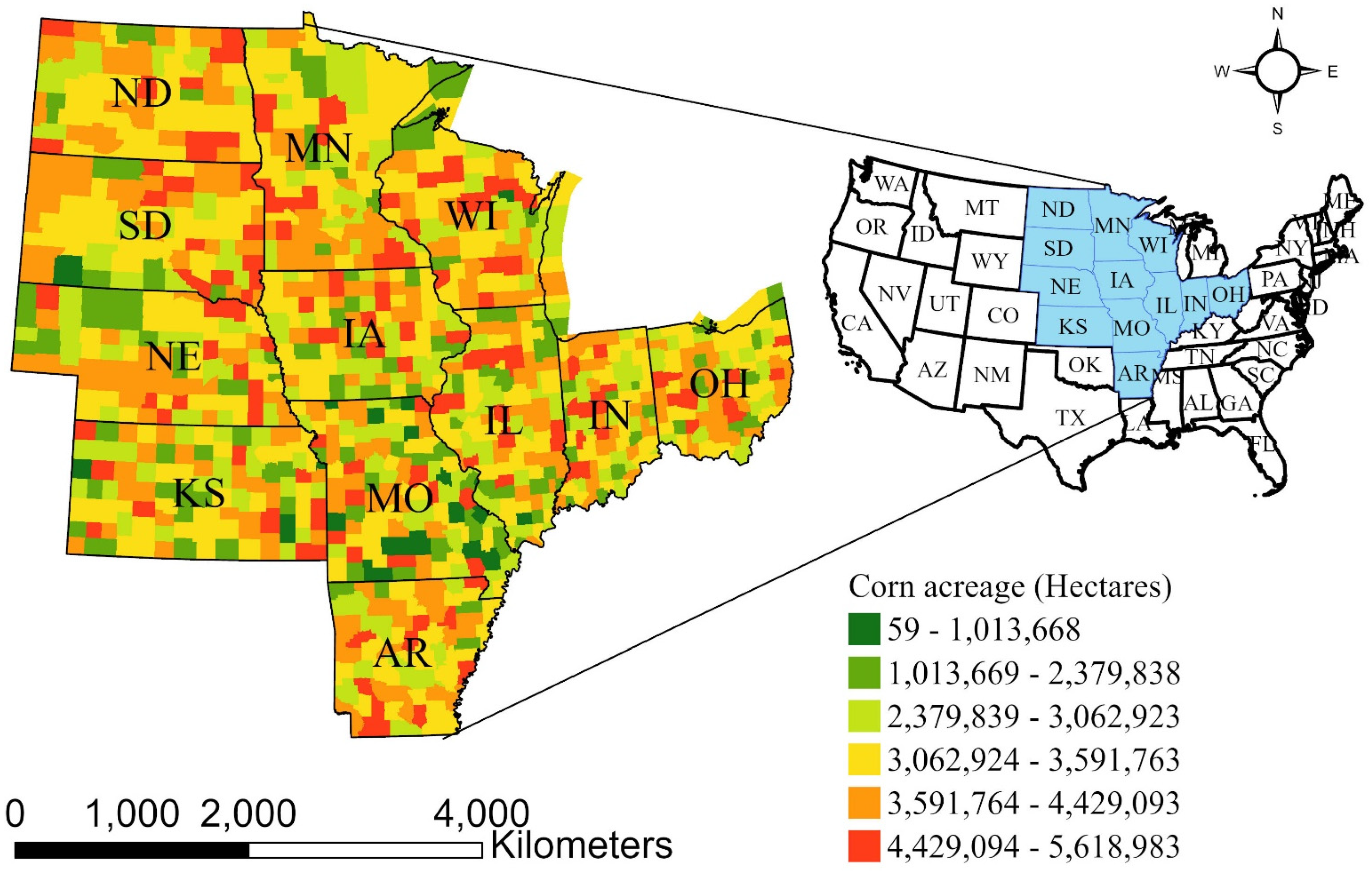
2.1. Study Area

This study was conducted in the US Corn Belt, which includes the following 12 Midwestern states: North Dakota (ND), South Dakota (SD), Nebraska (NE), Kansas (KS), Minnesota (MN), Iowa (IA), Missouri (MO), Arkansas (AR), Wisconsin (WI), Illinois (IL), Indiana (IN), and Ohio (OH) [2,52]. The US Corn Belt accounts for approximately 75% of corn production in the US [53] and 36% of global corn production [52]. The US accounts for approximately 15% of global corn export [1]. The corn acreage in the study area in 2020 is shown in Figure 1.

2.2. Datasets

The datasets used in this study are listed in Table 1. The details of each dataset are presented in subsequent sections.

2.2.1. Corn Yield Data

The corn yield data were collected from the National Agricultural Statistics Service Information (NASS), United States Department of Agriculture (USDA) [53]. The yield data were aggregated at the county level and are available to the public on their website (https://quickstats.nass.usda.gov, accessed on 18 November 2021). The county-level yield data have been used by many studies as the government provides most of the datasets at the county level [25,31,34,40]. County-level data from 2006 to 2020 were collected and mapped for each year using the geographic boundaries of the counties obtained from the US Census Topologically Integrated Geographic Encoding and Referencing (TIGER) project.

2.2.2. Cropland Data Layer

Cropland data layer (CDL) is a dataset published by USDA annually to provide information about croplands in the conterminous US (CONUS) [58]. CDL was initially available for several states, and it has covered the whole CONUS since 2008. CDL is available as a single GeoTIFF raster at a solution of 30 m and can be downloaded or used directly in the Google Earth engine (GEE) [59]. In this study, CDL was used to eliminate the pixels that are not corn to reduce interference of other crops. This is because the data for all variables are aggregated at the county level, and each county can contain pixels that are not corn. CDL was used as a mask for our study area so that only the data falling within corn fields are used.

2.2.3. Vegetation Indices

A wide range of remote sensing data are available to monitor global vegetation conditions [60]. The use of VIs is more popular because they can better reflect vegetation health conditions [44]. In this study, we use NDVI and EVI as the input for machine learning models. Equations (1) and (2) depict the mathematical formulae to calculate these two indices, respectively. NDVI characterizes the normalized difference between red and near-infrared (NIR) bands. It is very useful since vegetation strongly reflects NIR light and absorbs red light. The NDVI value for each pixel is between −1 and 1. Larger positive values represent increasing green vegetation, while negative values usually indicate nonvegetated surfaces [61,62]. EVI is another modified form of NDVI which can better model areas with large vegetation biomass and minimize the effects of soil and other atmospheric factors. C1 and C2 in Equation (2) represent the coefficients of the aerosol resistance term (C1 and C2 are 6 and 7.5, respectively, for the MODIS EVI product). In this study, we use a MODIS product [54] (NDVI and EVI), which has a spatial resolution of 250 m and a temporal resolution of 16 days [54]. We extracted NDVI and EVI from MOD13Q1.006 and used them because the MODIS data were consistent for our research period.
N D V I = N I R R e d / N I R + R e d
E V I = 2.5 × N I R R e d ( N I R + C 1 × R e d C 2 × B l u e + 1 )

2.2.4. Soil Data

Soil and its associated properties are vital to crop growth and can affect crop yield [26]. To conduct this study, we focus on 11 soil properties including cation exchange capacity (CEC), soil pH, soil available water content (AWC), soil available water storage (AWS), soil bulk density, soil organic carbon (SOC), clay content, sand content, saturated hydraulic conductivity, wilting point, and field capacity. The soil properties selected from the Soil Survey Geographic (SSURGO) database are based on their effects on crop yield and relevant literature [63,64,65]. These soil properties were derived using the 10 m gridded template compiled from the Gridded Soil Survey Geographic (gSSURGO) database.

2.2.5. Climate Data

The climatic variables used in this study were obtained from the Parameter elevation Relationships on Independent Slope Model (PRISM) [66]. The PRISM climate group collected data from many stations across the CONUS and used sophisticated methods to derive climate datasets. The PRISM data are provided at two spatial resolutions: 4 km and 800 m [57]. The 4 km PRISM data are available to the public. The climatic variables used in this study include precipitation, maximum temperature, minimum temperature, mean temperature, minimum vapor pressure deficit, maximum vapor pressure deficit, and mean dew point temperature. The climatic variables used in this study are based on previous studies [20,24,27,28,33]. The PRISM datasets have different temporal resolutions: daily, monthly, and yearly [67]. In this study, we utilized the daily PRISM data and aggregated them to derive 16-day composites since time-series NDVI and EVI data have a temporal resolution of 16 days [54].

2.3. Data Preprocessing

The datasets mentioned in Section 2.2.1, Section 2.2.2, Section 2.2.3, Section 2.2.4 and Section 2.2.5 have different spatial resolutions. All of these datasets were aggregated at the county level since the yield data provided by USDA are at the county level [40]. The datasets were filtered by including only those cells that are classified as corn in CDL, and the rest of the cells were excluded. The time-series predictors for remote sensing and climate data were aggregated to derive 16-day composites using GEE, which resulted in 12 time-series datasets for each predictor in the growing season (April to September). Eleven soil-related predictors mentioned in Section 2.2.4 were processed using ArcGIS Pro 2.8.0 [68] because soil data are not available in GEE. The data collected from GEE were further processed to remove missing and invalid values. The counties with no yield data were excluded from the analysis. The final dataset includes the data for 976 counties with a total of 12,372 records.

2.4. Methodology

In this research, we compare the results of the proposed GWRFR model with those of five widely used machine learning methods. All predictors are standardized. To predict corn yield in the US Corn Belt, the data were split into training and testing datasets. A 10-fold cross validation procedure is applied to tune the hyperparameters of models. For crop yield prediction, 5-fold and 10-fold cross validation techniques are generally used; however, for county-level corn yield prediction, 10-fold cross validation technique has been found effective [38]. For each model, the best fit model is applied to each test year to predict corn yield in that specific year. The R2 and RMSE for each test year are generated and reported along with the predicted results. The details on the machine learning models are presented below.

2.4.1. Multiple Linear Regression (MLR)

The foundation of machine learning regression is linear regression [69]. Ordinary least squares regression (OLS) is generally used for the estimation of coefficients of the relationship between several independent variables and the dependent variable. The relationship between a set of independent variables and dependent variable is assumed to be linear. If the regression process involves one independent variable, it is termed simple linear regression; if multiple independent variables are involved, it is termed multiple linear regression (MLR). The effect of each independent variable on the dependent variable is denoted in form of the coefficients in Equation (3):
y = β 0 + β 1 x 1 + β 2 x 2 + + β n x n + ε ,
where y represents the dependent variable, β n represents the coefficient of the independent variable x n , and ε is the error term associated with the model.
Linear regression is a widely used machine learning model due to its simplicity. However, there are some potential problems associated with it. First, linear models assume a linear relationship between the dependent variable and independent variables. This assumption might not be valid in every case. If the relationship between dependent variable and independent variable(s) is non-linear, linear regression models will have poor performance. Second, it is assumed that the error terms in linear models are always uncorrelated. If any correlation exists in the error terms, it can reduce the performance of linear models. It is assumed that linear models have a constant variance in the error terms (homoscedasticity), which is always not true [70]. Another major concern about using linear models is the presence of outliers and high leveraged points in the dataset which clearly affect the performance of linear models. Finally, it is assumed that the independent variables in the linear models are not correlated with each other (i.e., absence of multicollinearity in the datasets). The presence of multicollinearity in independent variables violates this assumption and reduces the performance of linear models.

2.4.2. Partial Least Square Regression (PLSR)

PLSR is a machine learning technique that can convert a large number of correlated predictors to a small number of uncorrelated predictors and then perform analysis on the reduced number of uncorrelated predictors [71]. As discussed above, we assume that the independent variables in linear regression models are not correlated with each other, and any presence of correlation can make linear regression models unsuitable for handling data with high dimensions and correlated independent variables. If there are more potential predictors and a possibility of multicollinearity in predictors, it is highly likely that MLR will have overfitting issues. In such cases, the model will have poor performance with new data [72]. PLSR characterizes the factors which can account for more variations in the dependent variable. PLSR is more focused on predicting the dependent variable (corn yield in this case) as compared to understanding the underlying relationship between independent variables (predictors) [73].

2.4.3. Support Vector Regression (SVR)

SVR is another machine learning model which is mainly used for regression problems [74]. SVR is a variation of the famous classification algorithm—support vector machines (SVM). The main difference between SVR and SVM is that SVR is used for regression while SVM is used for classification. In classification, SVM constructs a line or hyperplane which can divide the data into different classes. SVR gives us flexibility in terms of error tolerance and maximizing margins [75]. In SVR, the input is initially mapped using a linear or non-linear kernel function depending on relationship between predictors and response variables, after which a linear model is constructed to minimize the errors of the model.

2.4.4. Random Forest Regression (RFR)

RFR is based on the decision tree algorithm [76]. The main idea behind RFR is an ensemble of trees with each tree representing a randomly selected subset of variables and associated samples from the dataset. Generally, compared to decision trees, the performance of RFR is better since it creates multiple trees [77]. The results obtained from each tree are based on a majority vote of all associated trees. It is an ensemble of several regression trees, which is why it is sometimes called ensemble learning. The out-of-bag (OOB) performance estimation makes it well-suited for cross-validation and assessing performance. Another advantage of RF over other models is it performs better when data dimensions are high.

2.4.5. Geographically Weighted Random Forest Regression (GWRFR)

GWRFR is based on the traditional random forest algorithm and can handle spatial non-stationarity [51]. GWRFR is an ensemble learning method recently developed to improve non-spatial models. The main idea behind GWRFR is similar to GWR. GWRFR trains several local models instead of training a global model. However, it includes the power of the random forest regression model, which increases its predictive performance due to its non-parametric nature [50]. Linear models are influenced by outliers, and non-spatial models cannot model spatial heterogeneity [78]. GWRFR can overcome both weaknesses. Recently, GWRFR has been used in different applications such as socioeconomic risk factors analysis [79], type 2 diabetes prevalence analysis [80], and COVID-19 research [81]. GWRFR can be utilized to improve crop yield prediction since crop yield prediction is a spatial problem.

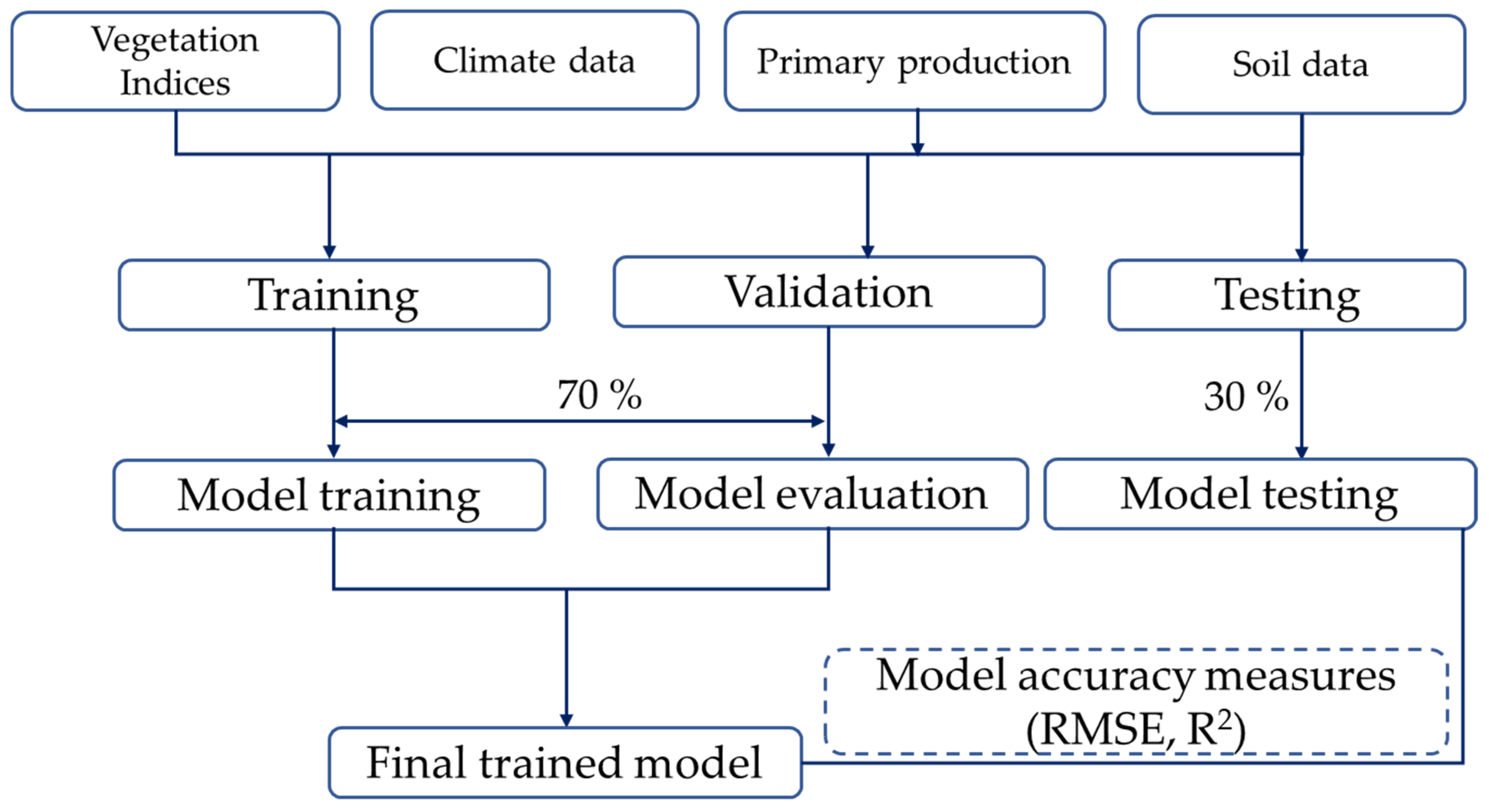
2.4.6. Experimental Design

After data preparation, we divided the data into training and testing datasets. The training dataset is used to train the model, while the testing dataset is used in model validation. Independent variables in this study are standardized using the standard scalar. The standard scalar rescales the distribution of the data so that the mean value becomes 0 and the standard deviation becomes 1. Feature scaling is an important step in machine learning as it reduces the undue influence of individual variables on the model [82]. Different independent variables have different scales, and sometimes large values influence models more than other values. Therefore, it is necessary to scale the independent variables before model construction to normalize their influence on models. For selecting the best hyperparameters for different machine learning models, a grid search with 10-fold cross validation was used to select the best parameters [38]. Mean squared error (MSE) was used as the criterion to select the best model. The models with the lowest MSE will be used for final predictions and evaluations. The experimental design is illustrated in Figure 2. The models trained in this study include MLR, PLSR, SVR, DTR, RFR, and GWRFR. We will compare the results of GWRFR with those of the other five machine learning algorithms.
We use (R2) and root mean squared error (RMSE) to assess model performance. The equations of R2 and RMSE are as follows:
R 2 = i = 1 n ( y i y ^ ) 2 ( y i y ¯ ) 2
R M S E = i = 1 n ( y i y ^ ) 2 n
One way to measure to what extent a model can capture spatial heterogeneity is to derive the spatial autocorrelation of the residuals [83]. Global Moran’s I statistics can be used to study spatial patterns [84]. Moran’s I value usually ranges from −1 to 1. A positive value represents positive autocorrelation, a negative value denotes negative autocorrelation, and a value close to zero indicates spatial randomness [84]. The presence of spatial autocorrelation in residuals suggests that the model is not able to consider the spatial effects [85]. Highly clustered values over space can bias predictions and result in large prediction errors [86]. We calculated spatial autocorrelation for the residuals of different models. The Moran’s I values of errors produced by non-spatial models such as MLR, PLSR, SVR, DTR, and RFR are compared with that of GWRFR to assess if GWRFR can better capture the spatial variability of corn yield in the US Corn Belt. For this study, if the Moran’s I values are closer to zero, the errors of the model are not clustered, which means the model can incorporate the spatial relationships [11].
Data preprocessing was performed using Python and the Jupyter Notebook [87] in Anaconda Version 3. Anaconda is a software distribution system that provides a package management system for Python and R. NumPy and GeoPandas libraries in Python were utilized for data preprocessing. The samples with incomplete information were eliminated using Pandas. To implement GWRFR, the SpatialML package in R was used, as this package was developed for spatially weighted machine learning algorithms [51]. Python and Scikit-learn [88] were used to implement the other five machine learning models. Scikit-learn provides a wide range of functionalities such as data standardization, model selection, data visualization, and model implementation. Finally, to derive the R2 of machine learning models, the r2score function in Scikit-learn was used in this research. To calculate the RMSE of the models, a new Python function was defined and used. We used the Matplotlib [89] and Seaborn [90] packages in Python to visualize the results of machine learning models. Finally, the Global Moran’s I tool in ArcGIS Pro 2.8.0 was used to examine spatial autocorrelation in residuals.

3. Results

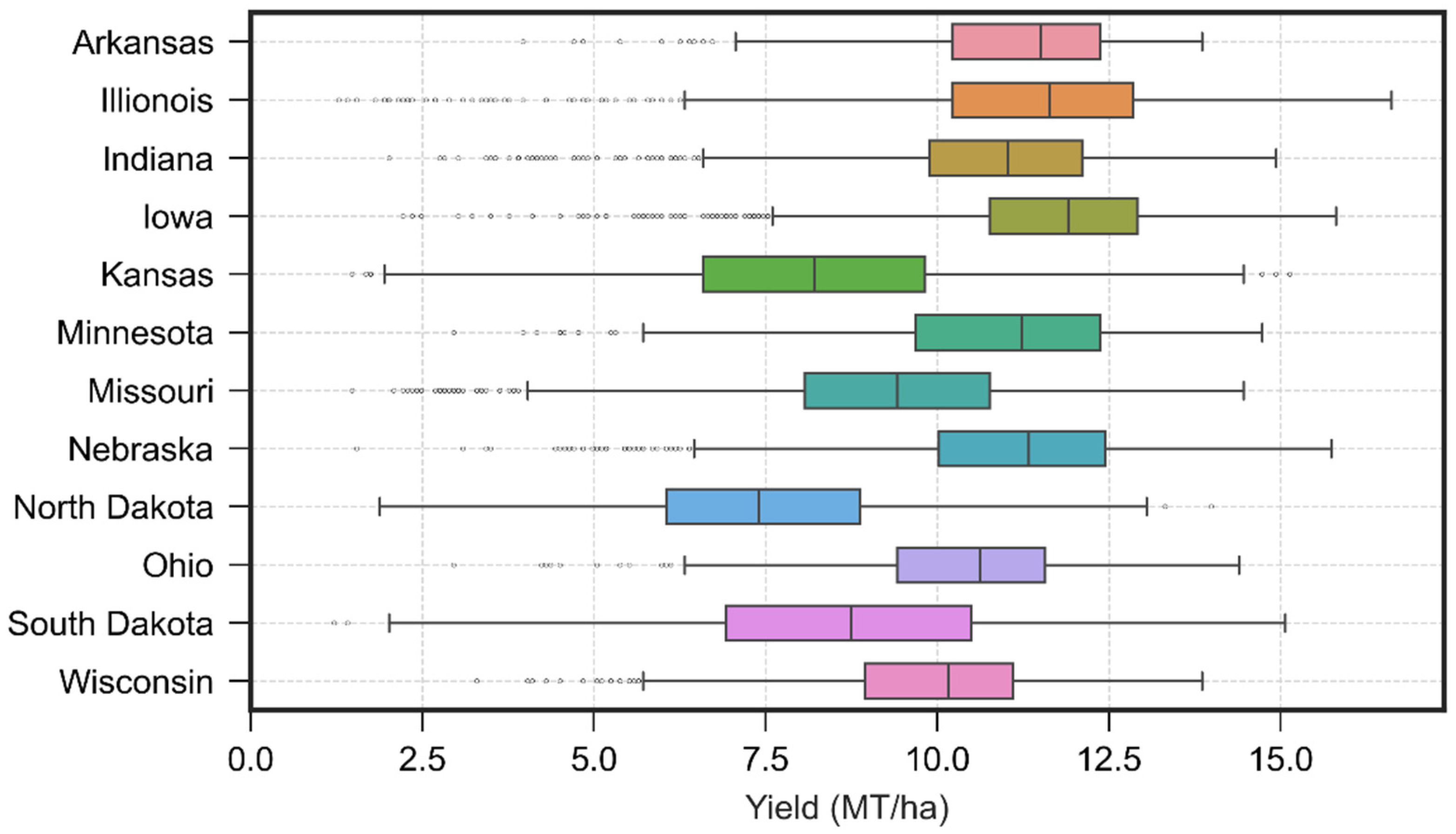
3.1. Descriptive Statistics

The corn yield data for all counties in the study area (2006–2020) range from 3.698 to 14.048 MT/ha with a mean value of 9.63 MT/ha and a standard deviation of 1.971 MT/ha (Table 2). The statistical distribution of the yield data is slightly negatively skewed. Table 2 also includes the descriptive statistics of the seven variables that are highly correlated with crop yield: GPP, NDVI, EVI, precipitation, mean dew point temperature (TD), maximum VPD, and minimum VPD. The GPP values range from 0.033 to 0.091 kg C/m2 with a mean of 0.072. The NDVI values during the research period range from 0.23 to 0.54 with a mean of 0.39. Figure 3 depicts the statistical distribution of corn yield in each state.

3.2. Model Performance with Different Sets of Input Features

In this study, the following five sets of features were used to test the performance of GWRFR and other machine learning models: (1) full-length features; (2) NDVI and EVI; (3) GPP; (4) climate data; and (5) soil data. We trained the six different models separately with each set of input features and used the R2 and RMSE to evaluate model performance. Figure 4 shows the spatial distribution of the predicted yield of (a) MLR, (b) PLSR, (c) SVR, (d) DTR, (e) DTR, and (f) RFR using (1) full-length features, (2) VIs, (3) GPP, (4) climate data, and (5) soil data. The overall spatial patterns of the predicted yield vary across different models and across different feature sets. Considerable spatial variation in the predicted yield can be observed across different models trained with soil data (a5–f5). For example, the predicted yields derived from the MLR and PLSR models trained with soil data (a5 and b5) differ considerably from the results of the other four models (c5–f5). Specifically, a5 and b5 have smaller yield values in the center of the study area and larger values in the northwest of the study area compared with c5–f5.

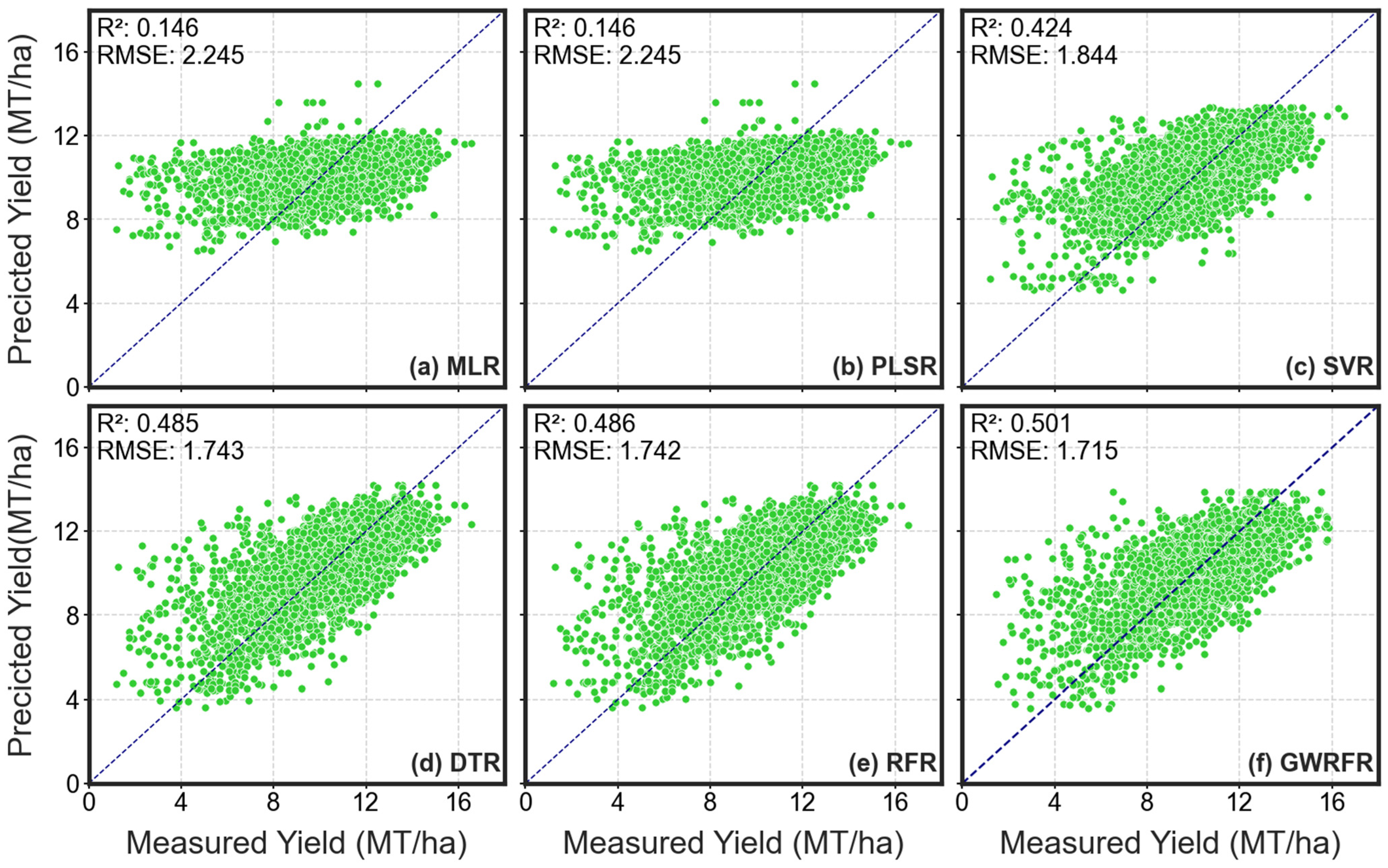
3.2.1. Full-Length Features

We trained all the six machine learning models with full-length features that include NDVI and EVI, GPP, climate variables (temperature, precipitation, VPD, and mean dew point temperature), and soil data. We present the R2 and RMSE of all six models in Figure 5. The derived R2 ranges from 0.791 to 0.901. The R2 and RMSE of GWRFR are 0.901 and 0.764 MT/ha, respectively. The results also illustrate that GWRFR outperforms other five models by 0.04–0.11 in terms of R2. DTR has the lowest performance (R2 = 0.743 and RMSE = 1.231 MT/ha). GWRFR improves the yield prediction by 0.073 in terms of R2 and 0.241 MT/ha in terms of the RMSE when compared with its non-spatial version, RFR (R2 = 0.828 and RMSE = 1.006 MT/ha). The scatterplots of the observed and predicted yield values are also presented in Figure 5. Overall, the yield predictions by machine learning models are more similar to the observed yield as most points follow the dotted blue line; however, there are some under- and over-estimations in different models. Such cases are rarely observed in GWRFR. DTR has the lowest performance when compared with other machine learning models because the points in its scatterplot are more dispersed.

3.2.2. Vegetation Indices

We predicted corn yield using time-series NDVI and EVI data and reported the R2 and RMSE of the models in Figure 6. The derived R2 ranges from 0.636 to 0.849. The R2 and RMSE of GWRFR are 0.849 and 0.944 MT/ha, respectively. The results also illustrate that GWRFR outperforms other models such as MLR, PLSR, SVR, DTR, and RFR by 0.10–0.21 in terms of R2. DTR has the lowest performance (R2 = 0.636 and RMSE = 1.466 MT/ha). GWRFR improves the yield prediction by 0.109 in terms of R2 and 0.294 MT/ha in terms of the RMSE when compared with its non-spatial version, RFR (R2 = 0.74 and RMSE = 1.238 MT/ha). The scatterplots of the observed and predicted yield values are presented in Figure 6. The performances of all machine learning algorithms including GWRFR decrease in this case when compared with that of the models using full-length features. More cases of underestimations and overestimations can be observed in the scatterplots; however, GWRFR can still perform better than other models.

3.2.3. Gross Primary Production

We further trained the six machine learning models using GPP data only. The time-series GPP data were used an independent variable to predict corn yield. We report the R2 and RMSE of the models in Figure 7. The derived R2 ranges from 0.553 to 0.839. The R2 and RMSE of GWRFR are 0.839 and 0.974 MT/ha, respectively. The results also illustrate that GWRFR outperforms other five models such as MLR, PLSR, SVR, DTR, and RFR by 0.144–0.286 in terms of R2. MLR and PLSR have a low performance (R2 = 0.553 and RMSE = 1.625 MT/ha). GWRFR improves yield prediction by 0.144 in terms of R2 and 0.367 MT/ha in terms of the RMSE when compared with its non-spatial version, RFR (R2 = 0.685 and RMSE = 1.341 MT/ha). The predictive performance of all machine learning algorithms including GWRFR is lower when compared with that of the models trained with full length features and VIs; however, the performance of GWRFR decreases only by 0.01 in terms of R2 and 0.03 MT/ha in terms of RMSE. The scatterplots of the observed and predicted yield values are also presented in Figure 7. As compared to previous feature sets, more under- and over-estimations can be observed in the scatterplots; however, GWRFR can still perform better than other models.

3.2.4. Climate Data

We further trained all six machine learning models using only climate-related variables. We report the R2 and RMSE of the models in Figure 8. The derived R2 ranges from 0.572 to 0.842. The R2 and RMSE of GWRFR are 0.842 and 0.967 MT/ha, respectively. The results also illustrate that GWRFR outperforms other models such as MLR, PLSR, SVR, DTR, and RFR by 0.03–0.27 in terms of R2. Again, MLR and PLSR have poor performance in terms of R2 (0.572 and 0.566, respectively) and RMSE (1.589 and 1.599 MT/ha, respectively). GWRFR improves the yield prediction by 0.03 in terms of R2 and 0.093 MT/ha in terms of the RMSE when compared with its non-spatial version, RFR (R2 = 0.809 and RMSE = 1.061 MT/ha). The scatterplots of the observed and predicted yield values are also presented in Figure 8. As compared to previous feature sets, more cases of underestimations and overestimations can be observed now in the scatterplots; however, GWRFR can still perform consistently better than other models.

3.2.5. Soil Data

Finally, we trained all six machine learning models to predict corn yield using soil data. Figure 9 shows the R2 and RMSE of the models. The derived R2 ranges from 0.146 to 0.501. The R2 and RMSE of GWRFR are 0.501 and 1.715 MT/ha, respectively. GWRFR again outperforms other models such as MLR, PLSR, SVR, DTR, and RFR by 0.015–0.355 in terms of R2. Again, MLR and PLSR have poor performance in terms of R2 (0.146) and RMSE (2.245 MT/ha). GWRFR improves the yield prediction by 0.015 in terms of R2 and by 0.0269 MT/ha in terms of RMSE when compared with its non-spatial version RFR (R2 = 0.486 and RMSE = 1.742 MT/ha). The scatterplots of the observed and predicted yield values are also presented in Figure 9. As compared to previous feature sets, more under- and over-estimations can be observed in the scatterplots, and model accuracy decreases significantly. GWRFR can still perform consistently better than other models.

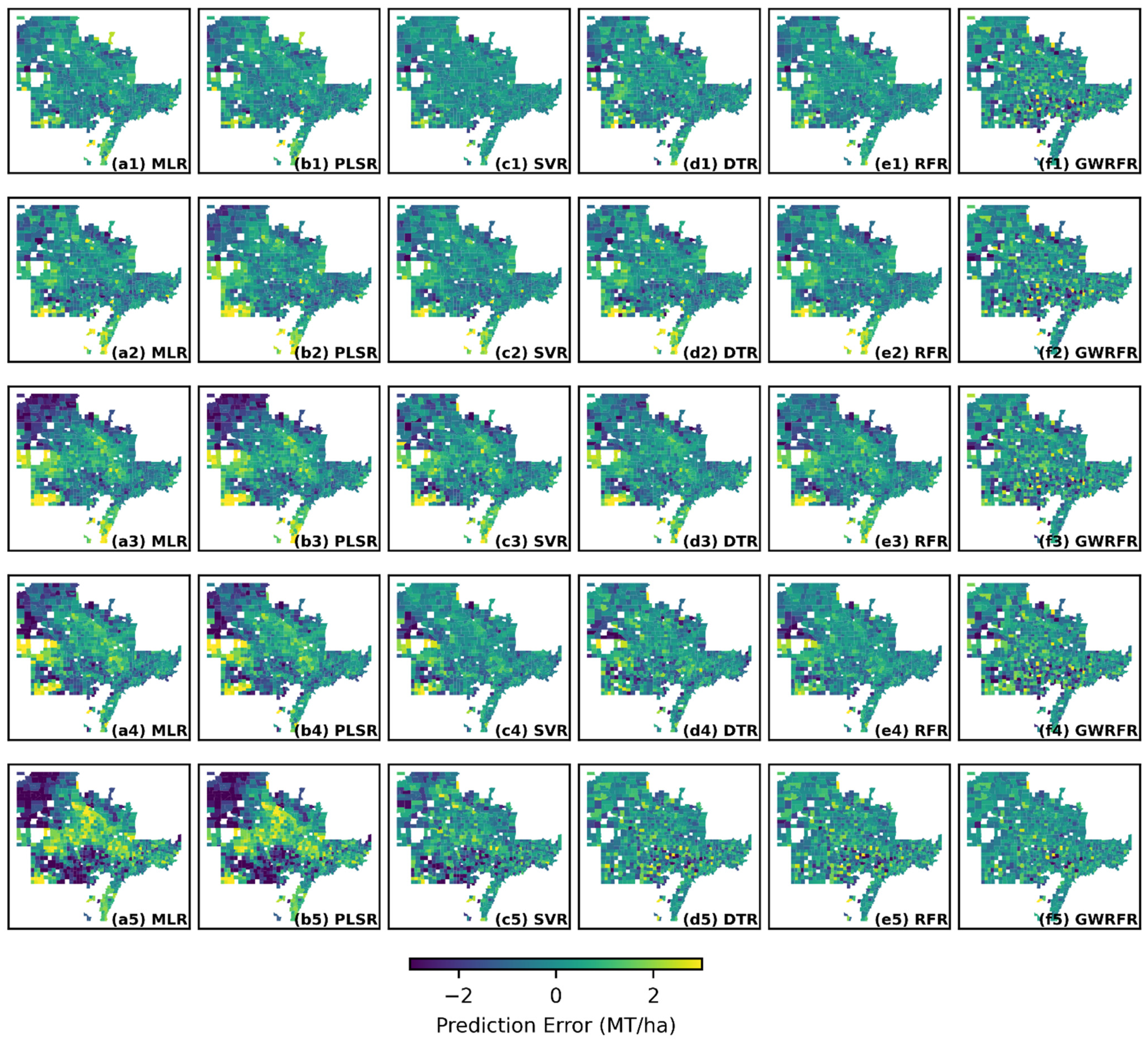
3.3. Spatial Autocorrelation in Residuals

We used Global Moran’s I to detect spatial autocorrelation in the prediction errors of all models to test if the models capture spatial heterogeneity [91,92]. Table 3 depicts the results of the Moran’s I analysis. In terms of spatial autocorrelation, the residuals of PLSR and SVR model are more clustered when compared with other non-spatial machine learning methods. However, GWRFR outperforms other models with the lowest Moran’s I value [11,93]. This means the errors are less clustered. Figure 10 illustrates the spatial distribution of prediction errors for all six models. The prediction errors of GWRFR are more randomly distributed as compared to non-spatial models. Smaller predictions errors are observed in the models trained with full-length features compared with those trained with other sets of features.

4. Discussion

This study addresses several important issues in building models for corn yield prediction. Our results demonstrate that model selection plays an important role in achieving more accurate yield predictions. We found that GWRFR performs better than other non-spatial machine learning algorithms. Nearby samples are more important than those distant ones in yield prediction at a specific location [51,81,85]. Our results are consistent with other studies that compared the performance of spatially weighted methods with that of non-spatial methods in crop yield prediction [11,29]. The Moran’s I values of residuals show that GWRFR can better capture spatial heterogeneity than traditional non-spatial models. Although GWRFR has a better performance than other models in county-level corn yield prediction in this study, more research needs to be conducted to evaluate its effectiveness in predicting the yield for other crops in other areas at different spatial scales. The performance of SVR trained with full length features and NDVI/EVI was second best; however, its performance gradually decreases when trained with GPP, climate data, and soil data. This shows that SVR can compete with GWRFR when full-length features or linearly correlated features (NDVI/EVI) are available.
Our results also show that feature selection is also very important in corn yield prediction. We observed the highest R2 and the lowest RMSE in the models trained with full length features. Our findings are consistent with previous studies [28,94] as the accuracy of machine learning models is heavily dependent on the training data. NDVI and EVI have been widely used in crop yield prediction [44]. VIs such as NDVI and EVI can reduce the noise in raw reflectance values [95] and provide vegetation-specific information for predicting corn yield. Moreover, VIs can be utilized in several other ways to improve the accuracy of machine learning models. For example, NDVI and EVI can be used to derive phenological information and the underlying environmental factors in different growth stages to further improve model performance [96,97]. Extreme climatic conditions can negatively impact crop yield and limit the predictive power of models if relevant data are not present. Furthermore, increased precipitation can have different impacts on crop yield depending on the spatio-temporal distribution of precipitation [98]. These additional factors affecting crop yield can only be addressed by including detailed climate data in the model training process. The overall performance of soil data is not very well compared with other categories of features such as VIs, GPP, and climate data. Furthermore, we found that time-series variables such as NDVI, GPP, and climate data can help improve model performance. This is because time-series features can better capture crop conditions in different stages of growth. Lastly, our study also has some limitations. County-level yield prediction involves the aggregation of yield and associated factors over a large area. Data aggregation can result in the loss of field-level or pixel-level information. Thus, further research needs to be conducted to examine if our findings can be used for field-level crop yield predictions. Moreover, several management factors such as plant density and planting dates also affect crop yield but were not included in this study. More research needs to be conducted to further examine the impacts of these factors on crop yield prediction.
Another aspect in crop yield prediction is data availability. Since VIs and GPP datasets are globally available and consistent in terms of spatial and temporal resolution, they can be used to construct scalable crop yield models. This can be useful for predicting yield in areas where data for other predictors such as soil and climate variables are not readily available [99]. Other datasets such as land surface temperature (LST) and solar-induced chlorophyll fluorescence (SIF) can also be used for crop yield prediction. Recent research has shown that replacing air temperature with MODIS LST can improve corn yield prediction [15]. Furthermore, the VI and GPP data used in this study have low spatial resolutions. Moderate-resolution multi-sensor data such as Sentinel-2 and Landsat-8 can also be used for yield prediction at the county level.

5. Conclusions

We investigated the performance of GWRFR in predicting corn yield at the county level in the US Corn Belt using different sets of features in this study. Our results show that GWRFR can outperform all other five non-spatial models in corn yield prediction irrespective of the features used. However, the predictive power of machine learning models varies significantly with the use of different sets of features. In addition to GWRFR, SVR and RFR have a better performance than other linear models. The models trained using full length features can yield better results than the same models trained using a subset of the features. GWRFR can model the spatial heterogeneity and produces the lowest Moran’s I value, which means GWRFR has the capability to address spatial heterogeneity and can be potentially used to address spatial problems in other applications. Although GWRFR outperforms other models in this study, more research needs to be conducted to test its effectiveness in predicting yield for other types of crops or in other areas.

Author Contributions

Conceptualization, S.N.K. and D.L.; methodology, S.N.K., D.L. and M.M.; software, S.N.K.; validation, D.L. and M.M.; formal analysis, S.N.K.; investigation, S.N.K.; resources, D.L.; data curation, S.N.K.; writing—original draft preparation, S.N.K.; writing—review and editing, D.L. and M.M.; visualization, S.N.K.; supervision, D.L.; project administration, D.L. All authors have read and agreed to the published version of the manuscript.

Funding

This research was jointly supported by the Department of Geography and Geospatial Sciences, South Dakota State University and the Higher Education Commission (HEC), Pakistan. The APC was funded by the Department of Geography and Geospatial Sciences, South Dakota State University.

Data Availability Statement

The data used in this study were mainly obtained from publicly available sources. The details about the datasets are available in Section 2.2.

Acknowledgments

The authors would like to acknowledge the information technology division of South Dakota State University, who provided the computing resources to process data and run models. Specifically, we would like to thank Rachael Auch for her technical support.

Conflicts of Interest

All authors declare no conflict of interest.

References

  1. Ranum, P.; Peña-Rosas, J.P.; Garcia-Casal, M.N. Global maize production, utilization, and consumption. Ann. N. Y. Acad. Sci. 2014, 1312, 105–112. [Google Scholar] [CrossRef] [PubMed]
  2. Green, T.R.; Kipka, H.; David, O.; McMaster, G.S. Where is the USA Corn Belt, and how is it changing? Sci. Total Environ. 2018, 618, 1613–1618. [Google Scholar] [CrossRef] [PubMed] [Green Version]
  3. Panagopoulos, Y.; Gassman, P.W.; Jha, M.K.; Kling, C.L.; Campbell, T.; Srinivasan, R.; White, M.; Arnold, J.G. A refined regional modeling approach for the Corn Belt–Experiences and recommendations for large-scale integrated modeling. J. Hydrol. 2015, 524, 348–366. [Google Scholar] [CrossRef] [Green Version]
  4. Pathak, T.B.; Maskey, M.L.; Dahlberg, J.A.; Kearns, F.; Bali, K.M.; Zaccaria, D. Climate change trends and impacts on California agriculture: A detailed review. Agronomy 2018, 8, 25. [Google Scholar] [CrossRef] [Green Version]
  5. Ehrlich, P.R.; Ehrlich, A.H.; Daily, G.C. Food security, population and environment. Popul. Dev. Rev. 1993, 19, 1–32. [Google Scholar] [CrossRef]
  6. Shahhosseini, M.; Martinez-Feria, R.A.; Hu, G.; Archontoulis, S.V. Maize yield and nitrate loss prediction with machine learning algorithms. Environ. Res. Lett. 2019, 14, 124026. [Google Scholar] [CrossRef] [Green Version]
  7. Ali, A.; Rondelli, V.; Martelli, R.; Falsone, G.; Lupia, F.; Barbanti, L. Management Zones Delineation through Clustering Techniques Based on Soils Traits, NDVI Data, and Multiple Year Crop Yields. Agriculture 2022, 12, 231. [Google Scholar] [CrossRef]
  8. Ahmad, W.; Iqbal, J.; Nasir, M.J.; Ahmad, B.; Khan, M.T.; Khan, S.N.; Adnan, S. Impact of land use/land cover changes on water quality and human health in district Peshawar Pakistan. Sci. Rep. 2021, 11, 16526. [Google Scholar] [CrossRef]
  9. Yuan, W.; Chen, Y.; Xia, J.; Dong, W.; Magliulo, V.; Moors, E.; Olesen, J.E.; Zhang, H. Estimating crop yield using a satellite-based light use efficiency model. Ecol. Indic. 2016, 60, 702–709. [Google Scholar] [CrossRef] [Green Version]
  10. Shahhosseini, M.; Hu, G.; Archontoulis, S. Forecasting corn yield with machine learning ensembles. Front. Plant Sci. 2020, 11, 1120. [Google Scholar] [CrossRef]
  11. Feng, L.; Wang, Y.; Zhang, Z.; Du, Q. Geographically and temporally weighted neural network for winter wheat yield prediction. Remote Sens. Environ. 2021, 262, 112514. [Google Scholar] [CrossRef]
  12. Iizumi, T.; Shin, Y.; Kim, W.; Kim, M.; Choi, J. Global crop yield forecasting using seasonal climate information from a multi-model ensemble. Clim. Serv. 2018, 11, 13–23. [Google Scholar] [CrossRef]
  13. Hunt, M.L.; Blackburn, G.A.; Carrasco, L.; Redhead, J.W.; Rowland, C.S. High resolution wheat yield mapping using Sentinel-2. Remote Sens. Environ. 2019, 233, 111410. [Google Scholar] [CrossRef]
  14. Rossato, L.; Alvalá, R.C.; Marengo, J.A.; Zeri, M.; Cunha, A.P.; Pires, L.; Barbosa, H.A. Impact of soil moisture on crop yields over Brazilian semiarid. Front. Environ. Sci. 2017, 5, 73. [Google Scholar] [CrossRef] [Green Version]
  15. Pede, T.; Mountrakis, G.; Shaw, S.B. Improving corn yield prediction across the US Corn Belt by replacing air temperature with daily MODIS land surface temperature. Agric. For. Meteorol. 2019, 276, 107615. [Google Scholar] [CrossRef]
  16. Cai, Y.; Guan, K.; Lobell, D.; Potgieter, A.B.; Wang, S.; Peng, J.; Xu, T.; Asseng, S.; Zhang, Y.; You, L. Integrating satellite and climate data to predict wheat yield in Australia using machine learning approaches. Agric. For. Meteorol. 2019, 274, 144–159. [Google Scholar] [CrossRef]
  17. Sabatino, L.; D’Anna, F.; Iapichino, G.; Moncada, A.; D’Anna, E.; De Pasquale, C. Interactive effects of genotype and molybdenum supply on yield and overall fruit quality of tomato. Front. Plant Sci. 2019, 9, 1922. [Google Scholar] [CrossRef] [Green Version]
  18. Imran, M.; Zurita-Milla, R.; Stein, A. Modeling Crop Yield in West-African Rainfed Agriculture Using Global and Local Spatial Regression. Agron. J. 2013, 105, 1177–1188. [Google Scholar] [CrossRef]
  19. Sellam, V.; Poovammal, E. Prediction of crop yield using regression analysis. Indian J. Sci. Technol. 2016, 9, 1–5. [Google Scholar] [CrossRef]
  20. Han, J.; Zhang, Z.; Cao, J.; Luo, Y.; Zhang, L.; Li, Z.; Zhang, J. Prediction of winter wheat yield based on multi-source data and machine learning in China. Remote Sens. 2020, 12, 236. [Google Scholar] [CrossRef] [Green Version]
  21. Petersen, L.K. Real-time prediction of crop yields from MODIS relative vegetation health: A continent-wide analysis of Africa. Remote Sens. 2018, 10, 1726. [Google Scholar] [CrossRef] [Green Version]
  22. Idso, S.B.; Jackson, R.D.; Reginato, R.J. Remote sensing for agricultural water management and crop yield prediction. Agric. Water Manag. 1977, 1, 299–310. [Google Scholar] [CrossRef]
  23. Schwalbert, R.A.; Amado, T.; Corassa, G.; Pott, L.P.; Prasad, P.V.; Ciampitti, I.A. Satellite-based soybean yield forecast: Integrating machine learning and weather data for improving crop yield prediction in southern Brazil. Agric. For. Meteorol. 2020, 284, 107886. [Google Scholar] [CrossRef]
  24. Brown, J.N.; Hochman, Z.; Holzworth, D.; Horan, H. Seasonal climate forecasts provide more definitive and accurate crop yield predictions. Agric. For. Meteorol. 2018, 260, 247–254. [Google Scholar] [CrossRef]
  25. Khaki, S.; Pham, H.; Wang, L. Simultaneous corn and soybean yield prediction from remote sensing data using deep transfer learning. Sci. Rep. 2021, 11, 11132. [Google Scholar] [CrossRef] [PubMed]
  26. Bruce, R.; Snyder, W.; Whiter, A., Jr.; Thomas, A.; Langdale, G. Soil variables and interactions affecting prediction of crop yield pattern. Soil Sci. Soc. Am. J. 1990, 54, 494–501. [Google Scholar] [CrossRef]
  27. Kern, A.; Barcza, Z.; Marjanović, H.; Árendás, T.; Fodor, N.; Bónis, P.; Bognár, P.; Lichtenberger, J. Statistical modelling of crop yield in Central Europe using climate data and remote sensing vegetation indices. Agric. For. Meteorol. 2018, 260, 300–320. [Google Scholar] [CrossRef]
  28. Li, Y.; Guan, K.; Yu, A.; Peng, B.; Zhao, L.; Li, B.; Peng, J. Toward building a transparent statistical model for improving crop yield prediction: Modeling rainfed corn in the US. Field Crops Res. 2019, 234, 55–65. [Google Scholar] [CrossRef]
  29. Imran, M.; Stein, A.; Zurita-Milla, R. Using geographically weighted regression kriging for crop yield mapping in West Africa. Int. J. Geogr. Inf. Sci. 2015, 29, 234–257. [Google Scholar] [CrossRef]
  30. Buckmaster, H.L. The Development of a Crop Yield Prediction Equation for Some Soils in the Blackland and Grand Prairies of Texas. Ph.D. Thesis, Texas A&M University, College Station, TX, USA, 1964. [Google Scholar]
  31. Ma, Y.; Zhang, Z.; Kang, Y.; Özdoğan, M. Corn yield prediction and uncertainty analysis based on remotely sensed variables using a Bayesian neural network approach. Remote Sens. Environ. 2021, 259, 112408. [Google Scholar] [CrossRef]
  32. Peng, B.; Guan, K.; Tang, J.; Ainsworth, E.A.; Asseng, S.; Bernacchi, C.J.; Cooper, M.; Delucia, E.H.; Elliott, J.W.; Ewert, F. Towards a multiscale crop modelling framework for climate change adaptation assessment. Nat. Plants 2020, 6, 338–348. [Google Scholar] [CrossRef] [PubMed]
  33. Leng, G.; Huang, M. Crop yield response to climate change varies with crop spatial distribution pattern. Sci. Rep. 2017, 7, 1463. [Google Scholar] [CrossRef] [PubMed]
  34. Roberts, M.J.; Braun, N.O.; Sinclair, T.R.; Lobell, D.B.; Schlenker, W. Comparing and combining process-based crop models and statistical models with some implications for climate change. Environ. Res. Lett. 2017, 12, 095010. [Google Scholar] [CrossRef]
  35. Parihar, C.M.; Jat, S.; Singh, A.; Ghosh, A.; Rathore, N.; Kumar, B.; Pradhan, S.; Majumdar, K.; Satyanarayana, T.; Jat, M. Effects of precision conservation agriculture in a maize-wheat-mungbean rotation on crop yield, water-use and radiation conversion under a semiarid agro-ecosystem. Agric. Water Manag. 2017, 192, 306–319. [Google Scholar] [CrossRef]
  36. Awad, M.M. Toward precision in crop yield estimation using remote sensing and optimization techniques. Agriculture 2019, 9, 54. [Google Scholar] [CrossRef] [Green Version]
  37. Wang, Y.; Zhang, Z.; Feng, L.; Du, Q.; Runge, T. Combining multi-source data and machine learning approaches to predict winter wheat yield in the conterminous united states. Remote Sens. 2020, 12, 1232. [Google Scholar] [CrossRef] [Green Version]
  38. Shahhosseini, M.; Hu, G.; Huber, I.; Archontoulis, S.V. Coupling machine learning and crop modeling improves crop yield prediction in the US Corn Belt. Sci. Rep. 2021, 11, 1606. [Google Scholar] [CrossRef]
  39. Mahlein, A.-K.; Oerke, E.-C.; Steiner, U.; Dehne, H.-W. Recent advances in sensing plant diseases for precision crop protection. Eur. J. Plant Pathol. 2012, 133, 197–209. [Google Scholar] [CrossRef]
  40. Sun, J.; Di, L.; Sun, Z.; Shen, Y.; Lai, Z. County-level soybean yield prediction using deep CNN-LSTM model. Sensors 2019, 19, 4363. [Google Scholar] [CrossRef] [Green Version]
  41. Ghosh, P.; Mandal, D.; Bhattacharya, A.; Nanda, M.K.; Bera, S. Assessing crop monitoring potential of Sentinel-2 in a spatio-temporal scale. Int. Arch. Photogramm. Remote Sens. Spat. Inf. Sci. 2018, 425, 227–231. [Google Scholar] [CrossRef] [Green Version]
  42. Zheng, Q.; Huang, W.; Cui, X.; Shi, Y.; Liu, L. New spectral index for detecting wheat yellow rust using Sentinel-2 multispectral imagery. Sensors 2018, 18, 868. [Google Scholar] [CrossRef] [PubMed] [Green Version]
  43. Wolanin, A.; Camps-Valls, G.; Gómez-Chova, L.; Mateo-García, G.; van der Tol, C.; Zhang, Y.; Guanter, L. Estimating crop primary productivity with Sentinel-2 and Landsat 8 using machine learning methods trained with radiative transfer simulations. Remote Sens. Environ. 2019, 225, 441–457. [Google Scholar] [CrossRef]
  44. Bannari, A.; Morin, D.; Bonn, F.; Huete, A. A review of vegetation indices. Remote Sens. Rev. 1995, 13, 95–120. [Google Scholar] [CrossRef]
  45. Liang, S. Comprehensive Remote Sensing; Elsevier: Amsterdam, The Netherlands, 2017. [Google Scholar]
  46. Mishra, S.; Mishra, D.; Santra, G.H. Applications of machine learning techniques in agricultural crop production: A review paper. Indian J. Sci. Technol. 2016, 9, 1–14. [Google Scholar] [CrossRef]
  47. Gilbertson, J.K.; Van Niekerk, A. Value of dimensionality reduction for crop differentiation with multi-temporal imagery and machine learning. Comput. Electron. Agric. 2017, 142, 50–58. [Google Scholar] [CrossRef]
  48. Ali, A.; Martelli, R.; Lupia, F.; Barbanti, L. Assessing multiple years’ spatial variability of crop yields using satellite vegetation indices. Remote Sens. 2019, 11, 2384. [Google Scholar] [CrossRef] [Green Version]
  49. Brunsdon, C.; Fotheringham, S.; Charlton, M. Geographically weighted regression. J. R. Stat. Soc. Ser. D (Stat.) 1998, 47, 431–443. [Google Scholar] [CrossRef]
  50. Santos, F.; Graw, V.; Bonilla, S. A geographically weighted random forest approach for evaluate forest change drivers in the Northern Ecuadorian Amazon. PLoS ONE 2019, 14, e0226224. [Google Scholar] [CrossRef]
  51. Georganos, S.; Grippa, T.; Niang Gadiaga, A.; Linard, C.; Lennert, M.; Vanhuysse, S.; Mboga, N.; Wolff, E.; Kalogirou, S. Geographical random forests: A spatial extension of the random forest algorithm to address spatial heterogeneity in remote sensing and population modelling. Geocarto Int. 2021, 36, 121–136. [Google Scholar] [CrossRef] [Green Version]
  52. Ort, D.R.; Long, S.P. Limits on yields in the corn belt. Science 2014, 344, 484–485. [Google Scholar] [CrossRef]
  53. NASS. NASS Quick Stats. In USDA National Agricultural Statistics Service (NASS). Available online: http://quickstats.nass.usda.gov (accessed on 19 December 2021).
  54. Didan, K. MOD13Q1 MODIS/Terra Vegetation Indices 16-Day L3 Global 250 m SIN Grid V006. NASA EOSDIS Land Processes DAAC; NASA: Washington, DC, USA, 2015.
  55. Running, S.W.; Zhao, M. User’s Guide Daily GPP and Annual NPP (MOD17A2/A3) Products NASA Earth Observing System MODIS Land Algorithm; The Numerical Terradynamic Simulation Group: Missoula, MT, USA, 2015. [Google Scholar]
  56. NRCS. Web Soil Survey. 2009. Available online: http://www.websoilsurvey.ncsc.usda.gov/app (accessed on 29 October 2017).
  57. Daly, C.; Bryant, K. The PRISM Climate and Weather System—An Introduction; PRISM Climate Group: Corvallis, OR, USA, 2013. [Google Scholar]
  58. Craig, M. A History of the Cropland Data Layer at NASS; Unpublished manuscript; Research and Development Division, USDA, NASS: Fairfax, VA, USA, 2010. [Google Scholar]
  59. Gorelick, N.; Hancher, M.; Dixon, M.; Ilyushchenko, S.; Thau, D.; Moore, R. Google Earth Engine: Planetary-scale geospatial analysis for everyone. Remote Sens. Environ. 2017, 202, 18–27. [Google Scholar] [CrossRef]
  60. Curran, P. Multispectral remote sensing of vegetation amount. Prog. Phys. Geogr. 1980, 4, 315–341. [Google Scholar] [CrossRef]
  61. Jackson, R.D.; Huete, A.R. Interpreting vegetation indices. Prev. Vet. Med. 1991, 11, 185–200. [Google Scholar] [CrossRef]
  62. Jensen, J.R. Introductory Digital Image Processing: A Remote Sensing Perspective, 4th ed.; Pearson: London, UK, 2015. [Google Scholar]
  63. Shearer, S.; Burks, T.; Fulton, J.; Higgins, S.; Thomasson, J.; Mueller, T.; Samson, S. Yield prediction using a neural network classifier trained using soil landscape features and soil fertility data. In Proceedings of the Annual International Meeting, Milwaukee, WI, USA, 9–12 July 2000; pp. 5–9. [Google Scholar]
  64. Khairunniza-Bejo, S.; Mustaffha, S.; Ismail, W.I.W. Application of artificial neural network in predicting crop yield: A review. J. Food Sci. Eng. 2014, 4, 1. [Google Scholar]
  65. Dahikar, S.S.; Rode, S.V. Agricultural crop yield prediction using artificial neural network approach. Int. J. Innov. Res. Electr. Electron. Instrum. Control. Eng. 2014, 2, 683–686. [Google Scholar]
  66. Daly, C.; Taylor, G.; Gibson, W.; Parzybok, T.; Johnson, G.; Pasteris, P. High-quality spatial climate data sets for the United States and beyond. Trans. ASAE 2000, 43, 1957. [Google Scholar] [CrossRef] [Green Version]
  67. Daly, C. Descriptions of PRISM Spatial Climate Datasets for the Conterminous United States; PRISM Climate Group: Corvallis, OR, USA, 2013; p. 14. [Google Scholar]
  68. ESRI. ArcGIS Pro (Version 2.8); ESRI Inc.: Redlands, CA, USA, 2020. [Google Scholar]
  69. Santiago, C.B.; Guo, J.-Y.; Sigman, M.S. Predictive and mechanistic multivariate linear regression models for reaction development. Chem. Sci. 2018, 9, 2398–2412. [Google Scholar] [CrossRef] [Green Version]
  70. Mei, C.-L.; Chen, F.; Wang, W.-T.; Yang, P.-C.; Shen, S.-L. Efficient estimation of heteroscedastic mixed geographically weighted regression models. Ann. Reg. Sci. 2021, 66, 185–206. [Google Scholar] [CrossRef]
  71. Geladi, P.; Kowalski, B.R. Partial least-squares regression: A tutorial. Anal. Chim. Acta 1986, 185, 1–17. [Google Scholar] [CrossRef]
  72. Hawkins, D.M. The problem of overfitting. J. Chem. Inf. Comput. Sci. 2004, 44, 1–12. [Google Scholar] [CrossRef] [PubMed]
  73. Tobias, R.D. An introduction to partial least squares regression. In Proceedings of the Twentieth Annual SAS Users Group International Conference, Orlando, FL, USA, 2–5 April 1995. [Google Scholar]
  74. Smola, A.J.; Schölkopf, B. A tutorial on support vector regression. Stat. Comput. 2004, 14, 199–222. [Google Scholar] [CrossRef] [Green Version]
  75. Li, G.; Wen, C.; Huang, G.-B.; Chen, Y. Error tolerance based support vector machine for regression. Neurocomputing 2011, 74, 771–782. [Google Scholar] [CrossRef]
  76. Smith, P.F.; Ganesh, S.; Liu, P. A comparison of random forest regression and multiple linear regression for prediction in neuroscience. J. Neurosci. Methods 2013, 220, 85–91. [Google Scholar] [CrossRef]
  77. Fawagreh, K.; Gaber, M.M.; Elyan, E. Random forests: From early developments to recent advancements. Syst. Sci. Control. Eng. 2014, 2, 602–609. [Google Scholar] [CrossRef] [Green Version]
  78. Schmidt, A.F.; Finan, C. Linear regression and the normality assumption. J. Clin. Epidemiol. 2018, 98, 146–151. [Google Scholar] [CrossRef] [Green Version]
  79. Luo, Y.; Yan, J.; McClure, S. Distribution of the environmental and socioeconomic risk factors on COVID-19 death rate across continental USA: A spatial nonlinear analysis. Environ. Sci. Pollut. Res. 2021, 28, 6587–6599. [Google Scholar] [CrossRef]
  80. Quiñones, S.; Goyal, A.; Ahmed, Z.U. Geographically weighted machine learning model for untangling spatial heterogeneity of type 2 diabetes mellitus (T2D) prevalence in the USA. Sci. Rep. 2021, 11, 6955. [Google Scholar] [CrossRef]
  81. Maiti, A.; Zhang, Q.; Sannigrahi, S.; Pramanik, S.; Chakraborti, S.; Cerda, A.; Pilla, F. Exploring spatiotemporal effects of the driving factors on COVID-19 incidences in the contiguous United States. Sustain. Cities Soc. 2021, 68, 102784. [Google Scholar] [CrossRef]
  82. Wan, X. Influence of feature scaling on convergence of gradient iterative algorithm. J. Phys. Conf. Ser. 2019, 1213, 032021. [Google Scholar] [CrossRef] [Green Version]
  83. Griffith, D.A. What is spatial autocorrelation? Reflections on the past 25 years of spatial statistics. L’Espace Géogr. 1992, 21, 265–280. [Google Scholar] [CrossRef]
  84. Overmars, K.d.; De Koning, G.; Veldkamp, A. Spatial autocorrelation in multi-scale land use models. Ecol. Model. 2003, 164, 257–270. [Google Scholar] [CrossRef]
  85. Cho, G. Spatial Processes: Models and Applications by AD Cliff and JK Ord. 16 by 24 em, 266 pages, maps, diags., index and bibliography. london: Pion Limited, 1981. (ISBN 08-85086-081-4). £ 20.50. Cartography 1983, 13, 59–60. [Google Scholar] [CrossRef]
  86. Gething, P.W.; Atkinson, P.M.; Noor, A.M.; Gikandi, P.W.; Hay, S.I.; Nixon, M.S. A local space–time kriging approach applied to a national outpatient malaria data set. Comput. Geosci. 2007, 33, 1337–1350. [Google Scholar] [CrossRef] [Green Version]
  87. Mendez, K.M.; Pritchard, L.; Reinke, S.N.; Broadhurst, D.I. Toward collaborative open data science in metabolomics using Jupyter Notebooks and cloud computing. Metabolomics 2019, 15, 125. [Google Scholar] [CrossRef] [Green Version]
  88. Pedregosa, F.; Varoquaux, G.; Gramfort, A.; Michel, V.; Thirion, B.; Grisel, O.; Blondel, M.; Prettenhofer, P.; Weiss, R.; Dubourg, V. Scikit-learn: Machine learning in Python. J. Mach. Learn. Res. 2011, 12, 2825–2830. [Google Scholar]
  89. Barrett, P.; Hunter, J.; Miller, J.T.; Hsu, J.-C.; Greenfield, P. Matplotlib—A Portable Python Plotting Package. In Proceedings of the Astronomical Data Analysis Software and Systems XIV, San Lorenzo de El Escorial, Spain, 2–5 October 2005; p. 91. [Google Scholar]
  90. Waskom, M.L. Seaborn: Statistical data visualization. J. Open Source Softw. 2021, 6, 3021. [Google Scholar] [CrossRef]
  91. Peralta, N.R.; Assefa, Y.; Du, J.; Barden, C.J.; Ciampitti, I.A. Mid-season high-resolution satellite imagery for forecasting site-specific corn yield. Remote Sens. 2016, 8, 848. [Google Scholar] [CrossRef] [Green Version]
  92. Maimaitijiang, M.; Sagan, V.; Sidike, P.; Hartling, S.; Esposito, F.; Fritschi, F.B. Soybean yield prediction from UAV using multimodal data fusion and deep learning. Remote Sens. Environ. 2020, 237, 111599. [Google Scholar] [CrossRef]
  93. Kumar, S.; Lal, R.; Liu, D. A geographically weighted regression kriging approach for mapping soil organic carbon stock. Geoderma 2012, 189, 627–634. [Google Scholar] [CrossRef]
  94. Mathieu, J.A.; Aires, F. Statistical weather-impact models: An application of neural networks and mixed effects for corn production over the United States. J. Appl. Meteorol. Climatol. 2016, 55, 2509–2527. [Google Scholar] [CrossRef]
  95. Khan, K.; Iqbal, J.; Ali, A.; Khan, S. Assessment of sentinel-2-derived vegetation indices for the estimation of above-ground biomass/carbon stock, temporal deforestation and carbon emissions estimation in the moist temperate forests of pakistan. Appl. Ecol. Environ. Res 2020, 18, 783–815. [Google Scholar] [CrossRef]
  96. Daryanto, S.; Wang, L.; Jacinthe, P.-A. Global synthesis of drought effects on maize and wheat production. PLoS ONE 2016, 11, e0156362. [Google Scholar] [CrossRef] [PubMed]
  97. Daryanto, S.; Wang, L.; Jacinthe, P.-A. Global synthesis of drought effects on cereal, legume, tuber and root crops production: A review. Agric. Water Manag. 2017, 179, 18–33. [Google Scholar] [CrossRef] [Green Version]
  98. Li, Y.; Guan, K.; Schnitkey, G.D. Excessive rainfall leads to comparable magnitude of corn yield loss as drought in the US. In Proceedings of the AGU Fall Meeting 2018, Washington, DC, USA, 10–14 December 2018. [Google Scholar]
  99. Yildirim, T.; Moriasi, D.N.; Starks, P.J.; Chakraborty, D. Using Artificial Neural Network (ANN) for Short-Range Prediction of Cotton Yield in Data-Scarce Regions. Agronomy 2022, 12, 828. [Google Scholar] [CrossRef]
Figure 1. The map of the study area (Corn acreage by county in 2020).
Remotesensing 14 02843 g001
Figure 2. Experimental design.
Remotesensing 14 02843 g002
Figure 3. State-wise corn yield distributions in the US Corn Belt (2006–2020).
Remotesensing 14 02843 g003
Figure 4. The spatial distribution of predicted yield of (a) MLR, (b) PLSR, (c) SVR, (d) DTR, (e) RFR, and (f) GWRFR using (1) full-length features, (2) vegetation indices derived from RS data, (3) GPP, (4) climate data, and (5) soil data.
Remotesensing 14 02843 g004
Figure 5. The scatterplots of the actual yield and the predicted yield derived from (a) MLR, (b) PLSR, (c) SVR, (d) DTR, (e) RFR, and (f) GWRFR using full-length features.
Remotesensing 14 02843 g005
Figure 6. The scatterplots of the actual yield and the predicted yield derived from (a) MLR, (b) PLSR, (c) SVR, (d) DTR, (e) RFR, and (f) GWRFR using only vegetation indices derived from RS data.
Remotesensing 14 02843 g006
Figure 7. The scatterplots of the actual yield and the predicted yield derived from (a) MLR, (b) PLSR, (c) SVR, (d) DTR, (e) RFR, and (f) GWRFR using only GPP data.
Remotesensing 14 02843 g007
Figure 8. The scatterplots of actual yield and predicted yield derived from (a) MLR, (b) PLSR, (c) SVR, (d) DTR, (e) RFR, and (f) GWRFR using only climate data.
Remotesensing 14 02843 g008
Figure 9. The scatterplots of actual yield and predicted yield derived from (a) MLR, (b) PLSR, (c) SVR, (d) DTR, (e) RFR, and (f) GWRFR using only soil data.
Remotesensing 14 02843 g009
Figure 10. The spatial distribution of prediction errors of (a) MLR, (b) PLSR, (c) SVR, (d) DTR, (e) RFR, and (f) GWRFR using (1) full-length features, (2) vegetation indices derived from RS data, (3) GPP, (4) climate data, and (5) soil data.
Remotesensing 14 02843 g010
Table 1. The datasets used in the study.
DataVariablesUnitSourceSpatial Resolution
Satellite data [54]Normalized difference vegetation index (NDVI)-MODIS250 m
Enhanced vegetation index (EVI)-MODIS250 m
Primary production [55]Gross primary production (GPP)kg C/m2MODIS500 m
Soil [56]Available water content (AWC)cmgSSURGO 10 m
Available water storage (AWS)mmgSSURGO10 m
Cation exchange capacity (CEC)meq/100 ggSSURGO10 m
Bulk densityg/cm3gSSURGO10 m
Percent clayPercentgSSURGO10 m
Percent sandPercentgSSURGO10 m
Field capacitycm/cmgSSURGO10 m
Organic carbong C/m2gSSURGO10 m
pH-gSSURGO10 m
Saturated hydraulic conductivityμm/secgSSURGO10 m
Wilting pointcm/cmgSSURGO10 m
Climate [57]PrecipitationmmPRISM4 km
Minimum temperature°CPRISM4 km
Maximum temperature°CPRISM4 km
Mean temperature°CPRISM4 km
Minimum vapor pressure deficithPaPRISM4 km
Maximum vapor pressure deficithPaPRISM4 km
Mean dew point temperature°CPRISM4 km
MODIS: Moderate resolution imaging spectroradiometer. gSSURGO: Gridded soil survey geographic database. PRISM: Parameter-elevation regressions on independent slopes model.
Table 2. The descriptive statistics of the seven features related to corn yield.
Yield (MT/ha)GPP (kg C/m2)NDVIEVIPrecipitation (mm)Mean TD (°C)Max VPD (hPa)Min VPD (hPa)
Minimum3.6980.0330.230.331.546.3111.980.34
Maximum14.0480.0910.540.764.9118.9533.283..45
Mean9.63760.0720.390.533.3512.5318.731.28
SD1.9710.0100.050.060.602.403.390.39
NDVI: Normalized difference vegetation index. EVI: Enhanced vegetation index. Mean TD: Mean dew point temperature. VPD: Vapor pressure deficit. SD: Standard deviation.
Table 3. Moran’s I value of residuals for MLR, PLSR, SVR, DTR, RFR, and GWRFR.
ModelMoran’s IZ Scorep-Value
MLR0.27721.280.00
PLSR0.29521.340.00
SVR0.29522.600.00
DTR0.27721.380.00
RFR0.26920.610.00
GWRFR0.13910.680.00
Publisher’s Note: MDPI stays neutral with regard to jurisdictional claims in published maps and institutional affiliations.

