Convolutional Neural Networks for Automated Built Infrastructure Detection in the Arctic Using Sub-Meter Spatial Resolution Satellite Imagery

Abstract

Rapid global warming is catalyzing widespread permafrost degradation in the Arctic, leading to destructive land-surface subsidence that destabilizes and deforms the ground. Consequently, human-built infrastructure constructed upon permafrost is currently at major risk of structural failure. Risk assessment frameworks that attempt to study this issue assume that precise information on the location and extent of infrastructure is known. However, complete, high-quality, uniform geospatial datasets of built infrastructure that are readily available for such scientific studies are lacking. While imagery-enabled mapping can fill this knowledge gap, the small size of individual structures and vast geographical extent of the Arctic necessitate large volumes of very high spatial resolution remote sensing imagery. Transforming this ‘big’ imagery data into ‘science-ready’ information demands highly automated image analysis pipelines driven by advanced computer vision algorithms. Despite this, previous fine resolution studies have been limited to manual digitization of features on locally confined scales. Therefore, this exploratory study serves as the first investigation into fully automated analysis of sub-meter spatial resolution satellite imagery for automated detection of Arctic built infrastructure. We tasked the U-Net, a deep learning-based semantic segmentation model, with classifying different infrastructure types (residential, commercial, public, and industrial buildings, as well as roads) from commercial satellite imagery of Utqiagvik and Prudhoe Bay, Alaska. We also conducted a systematic experiment to understand how image augmentation can impact model performance when labeled training data is limited. When optimal augmentation methods were applied, the U-Net achieved an average F1 score of 0.83. Overall, our experimental findings show that the U-Net-based workflow is a promising method for automated Arctic built infrastructure detection that, combined with existing optimized workflows, such as MAPLE, could be expanded to map a multitude of infrastructure types spanning the pan-Arctic.

1. Introduction

Permafrost, defined as Earth materials that remain at or below 0 °C for at least two consecutive years, underlies approximately 24% of the exposed land surface of the Northern Hemisphere [1]. However, climate change has led to widespread warming of the permafrost landscapes across the Arctic [2], where land surface temperatures are reported to have increased by more than 0.5 °C per decade since 1981, exceeding average global warming by a factor of between 2 and 3 [3]. This rapid warming causes degradation of permafrost that, if ice-rich, results in destructive processes such as differential land-surface subsidence [4]. Consequently, built infrastructure (e.g., roads and railroads, fuel and water pipelines, residential and public buildings, industrial facilities, airports, etc.) across the Arctic are at risk of structural failure [5,6,7]. Climate change projections under the RCP8.5 scenario show that infrastructure built upon permafrost will be subject to decreases in foundation bearing capacity and land-surface subsidence by 2050, resulting in a large financial cost of infrastructure repair and adaptation [8,9].

Furthermore, the potential for widespread infrastructure failure is linked to a range of consequences, including risks to society and public health, economic development, and industrial activity. Approximately 3.3 million people populating the Arctic permafrost landscapes [10], representing smaller indigenous settlements to larger industrial cities, live in areas where permafrost will degrade and disappear by 2050. Therefore, the livelihood and sustainable development of communities are threatened by the vulnerability of infrastructure to permafrost degradation [7,11,12]. Additionally, the increasing economic relevance of the Arctic due to natural resource extraction [13] has driven the expansion of industrial infrastructure, such as oil and gas facilities, pipelines, and supply roads, across highly sensitive permafrost, increasing the risk of negative impacts extending beyond the Arctic region [14]. However, infrastructure expansion itself has been recognized to contribute to localized permafrost degradation along with global warming [15,16,17,18].

The vulnerability of Arctic infrastructure to the destructive effects of permafrost degradation has been acknowledged by the scientific community, which is calling for pan-Arctic infrastructure risk assessments [19]. Frameworks to perform such pan-Arctic assessments have recently been designed and implemented, utilizing geospatial data to account for the location, extent, and type of infrastructure features. Ramage et al. [10] utilized point features to represent the locations of settlements with available population data to assess the number of settlements and people located in high-hazard zones. Suter et al. [9] estimated the cost of infrastructure damage due to permafrost degradation, merging governmental and open-source datasets to represent linear infrastructure, including roads, railroads, and pipelines as line features and buildings, airports, and ports as point features. Hjort et al. [5] identified hazard zones and quantified the risk of damage to infrastructure, utilizing OpenStreetMap data to represent major roads as line features and buildings as point features.

The major challenge for these studies was access to a consistent, accurate, and detailed high spatial resolution geospatial dataset of Arctic built infrastructure. For example, while OpenStreetMap is globally available, large areas of the Arctic are missing from it, namely areas with recent industrial development, and data quality is inconsistent [5]. Other global landcover datasets exist, such as the Global Man-made Impervious Surface dataset [20] and the Human Built-up and Settlement Extent dataset [21]. However, these are based on 30 m Landsat imagery and therefore can only document the general extent and location of impervious surfaces and built-up areas with no subcategorization of features, limiting their value to risk assessment frameworks. As a result, publicly available sources (national and local data, open-source projects) must be merged to achieve pan-Arctic coverage as demonstrated in the aforementioned studies, leading to inconsistencies among heterogeneous datasets.

Satellite-based mapping can be used to improve the geospatial data record of pan-Arctic built infrastructure. While we cannot guarantee it is completely exhaustive, we conducted a literature survey on Arctic built infrastructure mapping efforts and found that the task is ill-addressed, with few studies existing and only one study addressing pan-Arctic mapping from recent satellite imagery. The survey results are summarized in

Table 1. Literature survey on satellite-based Arctic built infrastructure mapping efforts.

Reference	Study Area	Data	Spatial Resolution (in Order of Listed Data, “Field Survey” Omitted)	Method	Feature(s) of Interest
Kumpula et al., 2006 [25]	Bovanenkovo gas field, Yamal Peninsula (West Siberia)	Field survey, QuickBird-2 (panchromatic, multispectral), ASTER VNIR, Landsat (TM, MSS)	0.61 m, 2.5 m, 15 m, 30 m, 80 m	Manual digitization	Quarries, power lines, roads, winter roads, drill towers, barracks
Kumpula et al., 2010 [26]	Bovanenkovo gas field, Yamal Peninsula (West Siberia)	Field survey, QuickBird-2 (pan, multi), ASTER VNIR, SPOT (pan, multi), Landsat (ETM7, TM, MSS)	0.63 m, 2.4 m, 15 m, 10 m, 20 m, 30 m, 30 m, 80 m	Manual digitization	Roads, impervious cover, barracks, winter roads, settlements, quarries
Kumpula et al., 2011 [27]	Bovanenkovo gas field and Toravei oil field, Yamal Peninsula (West Siberia)	Field survey, QuickBird-2 (pan, multi), ASTER VNIR, SPOT (multi), Landsat (ETM7, TM, MSS)	0.63 m, 2.4 m, 15 m, 10 m, 20 m, 30 m, 30 m	Manual digitization	Buildings, roads, sand quarries, pipelines
Kumpula et al., 2012 [23]	Bovanenkovo gas field, Yamal Peninsula (West Siberia)	Field survey, QuickBird-2 (pan, multi), GeoEye, ASTER VNIR, SPOT (multi), Landsat (ETM7, TM, MSS)	0.63 m, 2.4 m, 1.65 m, 15 m, 20 m, 30 m, 30 m, 70 m	Manual digitization	Pipelines, powerlines, drilling towers, roads, impervious cover, barracks, settlements, quarries
Raynolds et al., 2014 [16]	Prudhoe Bay Oilfield, Alaska	Aerial photography (B&W, color, color infrared)	1 ft resolution for two images. Map scale was then used to describe the rest of the imagery. Scales are as follows: 1:3000, 1:6000, 1:12,000, 1:18,000, 1:24,000, 1:60,000, 1:68,000, 1:120,000	Manual digitization	Roads, gravel pads, excavations, pipelines, powerlines, fences, canals, gravel and construction debris
Gadal and Ouerghemmi, 2019 [28]	Yakutsk, Russia	SPOT-6 (pan, multi), Sentinel-2 (multi)	1.5 m, 6 m, 10 m	Semi-automated (object-based image analysis)	Houses, other structures
Ourng et al., 2019 [29]	Surgut, Russia	Sentinel-1 (SAR), Sentinel-2 (multi), Landsat (TM, MSS)	10 m, 10 m, 30 m, 60 m	Automated (machine learning)	Built-up area
Bartsch et al., 2020 [22]	Pan-Arctic, within 100 km of the Arctic coast	Sentinel-1 (SAR) and Sentinel-2 (multi)	10 m, 10 m	Automated (machine learning and deep learning)	Buildings, roads, other human-impacted areas
Ardelean et al., 2020 [24]	Bovanenkovo gas field, Yamal Peninsula (West Siberia)	QuickBird-2 (pan, multi), GeoEye-1 (pan, multi)	0.6 m, 2.4 m, 0.4 m, 1.8 m	Manual digitization	Buildings, roads

. Based on this survey, it was found that most studies mapped built infrastructure across small geographic extents through manual digitization, with a focus on studying anthropogenic change in the Bovanenkovo gas field in the Yamal Peninsula, Russia. Bartsch et al. [22] presents the sole product derived from automated mapping on the pan-Arctic scale, providing the first pan-Arctic satellite-based record of expanding infrastructure and anthropogenic impacts along all permafrost-affected coasts. However, this study is limited to the use of Sentinel-1 and Sentinel-2 satellite imagery, which only provides medium spatial resolution at 10 m, and to a region within 100 km of the Arctic coast. It has been noted that very high spatial resolution (VHSR) imagery (<5 m resolution) is crucial in providing the required level of detail for accurate detection and classification of individual structures in the Arctic [22,23,24]. Therefore, the use of medium-resolution imagery means that many features can be missed, and those that are detected cannot be subcategorized. Despite this, all of the published products had limited access to VHSR imagery due to high imagery costs and low availability. However, the entire Arctic has been imaged by Maxar commercial satellite sensors at a sub-meter resolution, providing free ‘big’ imagery data to U.S. National Science Foundation Polar Program-funded researchers via the Polar Geospatial Center at the University of Minnesota.

The conspicuous shortfalls of traditional remote sensing image analysis when confronted with large volumes of VHSR imagery [30] have catalyzed a migration towards computer vision-based algorithms, namely the convolutional neural network (CNN). High spatial resolution images present scene objects much larger than the associated pixel size, introducing complex properties such as geometry, context, pattern, and texture that compose objects at multiple levels. Furthermore, higher spatial resolution significantly increases intra-class spectral variability, given the increased number of pixels constructing image features [31]. As such, traditional image analysis methods, namely per-pixel-based approaches, are ill-equipped to handle VHSR imagery, whereas CNNs are better equipped. For example, urban area extraction from coarse spatial resolution imagery may be satisfied by an algorithm that solely exploits high reflectance in the near-infrared region (which is characteristic of urban areas). However, as individual urban structures become visible at finer resolutions, detecting these objects will require an algorithm that can exploit features beyond the spectral reflectance values, such as edges, corners, and curves of buildings and roads, geometric patterns visible on building rooftops, textural differences between human-built structures and natural landscape backgrounds, etc. Through several processing layers, CNNs can learn to optimize the convolutional filters required to extract these features at multiple levels of abstraction, which are then assembled into feature representations used to detect and classify scene objects.

Several studies have successfully implemented CNN algorithms, namely the Mask R-CNN and the U-Net, for automated detection of various kinds of built infrastructure from VHSR imagery at multiple scales. The Mask R-CNN performs object instance segmentation, in which each individual object associated with a given class is detected, delineated with a bounding box, and classified [32]. The U-Net performs semantic segmentation, in which each pixel in an image is classified based on the detected object it is associated with. However, while object instance segmentation would treat, for example, multiple buildings of the same type as distinct structures, semantic segmentation would treat them as a single entity and therefore does not count the number of individual structures. Therefore, training the Mask R-CNN is more computationally intensive than training the U-Net, but both have recently achieved favorable results in infrastructure detection from high spatial resolution remote sensing imagery. For example, Tiede et al. tasked a Mask R-CNN with detecting dwellings in Khartoum, Sudan, from 0.5 m Pléiades satellite imagery, achieving an F1 score of 0.78 [33]. Wang et al. used an improved Mask R-CNN to detect rural buildings with different roof types in Hunan Province, China, from high-resolution UAV imagery, reaching an F1 score of 0.788 [34]. Li et al. demonstrated U-Net-based semantic segmentation for building footprint extraction from WorldView-3 satellite imagery of Las Vegas, Paris, Shanghai, and Khartoum, achieving an F1 score of 0.704 [35]. Yang et al. tasked a modified U-Net with extracting roads from aerial imagery in the Massachusetts Roads dataset and DeepGlobe Road Extraction dataset, achieving F1 scores of 0.784 and 0.794, respectively [36]. However, deep learning-based infrastructure detection from VHSR imagery has so far not been tested in the Arctic.

In this paper, we present the first study on CNN-based automated detection of built infrastructure at two Arctic locations using VHSR imagery. Our overall objective was to understand the ability of the U-Net CNN to perform semantic segmentation of sub-meter-resolution satellite imagery for detection of built infrastructure in the Arctic. Target classes included residential and commercial buildings, public buildings, industrial buildings, and roads. Additionally, we conducted a systematic experiment to understand how image augmentation improves the performance of the U-Net CNN when training data is limited.

2. Materials and Methods

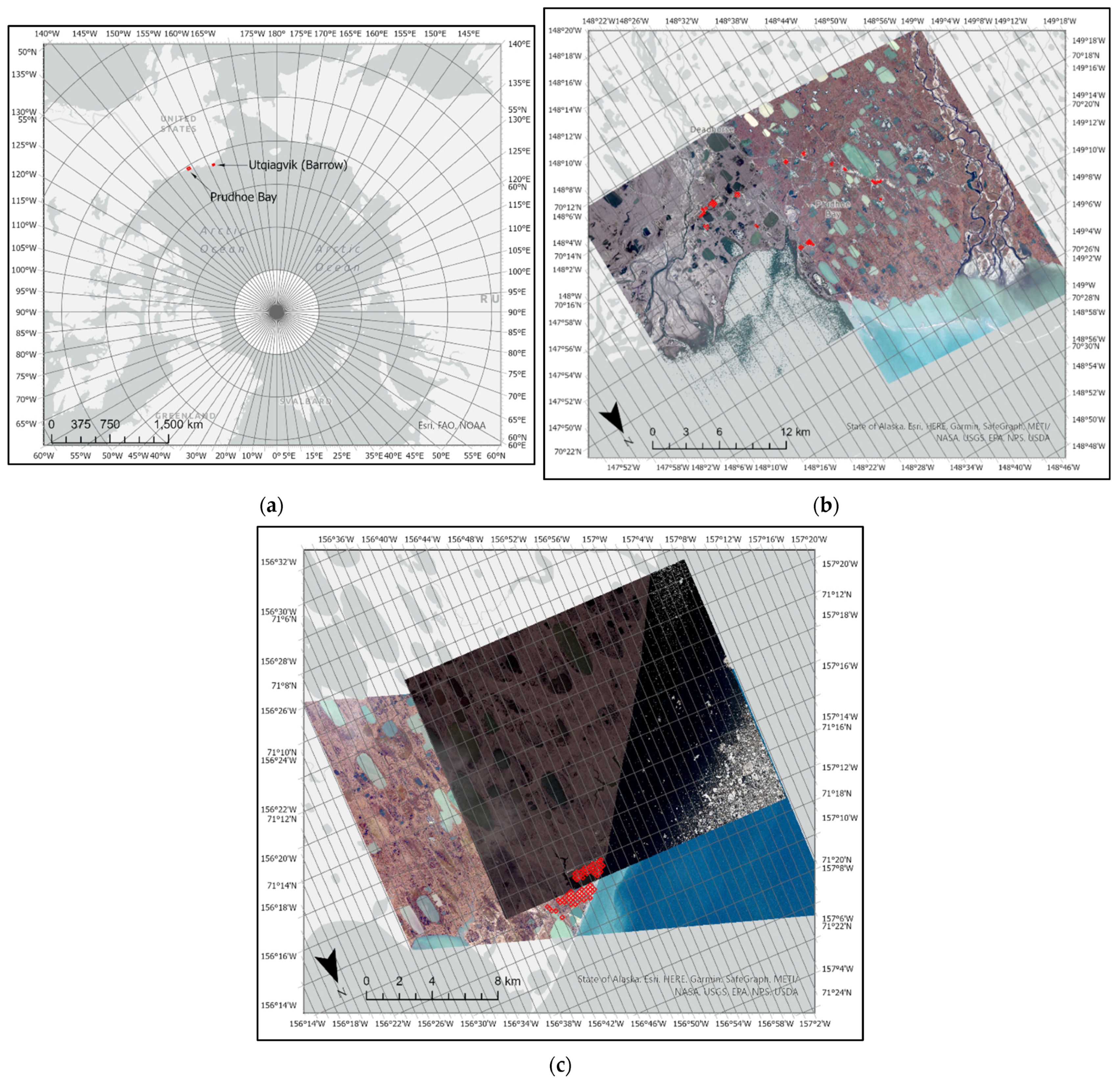
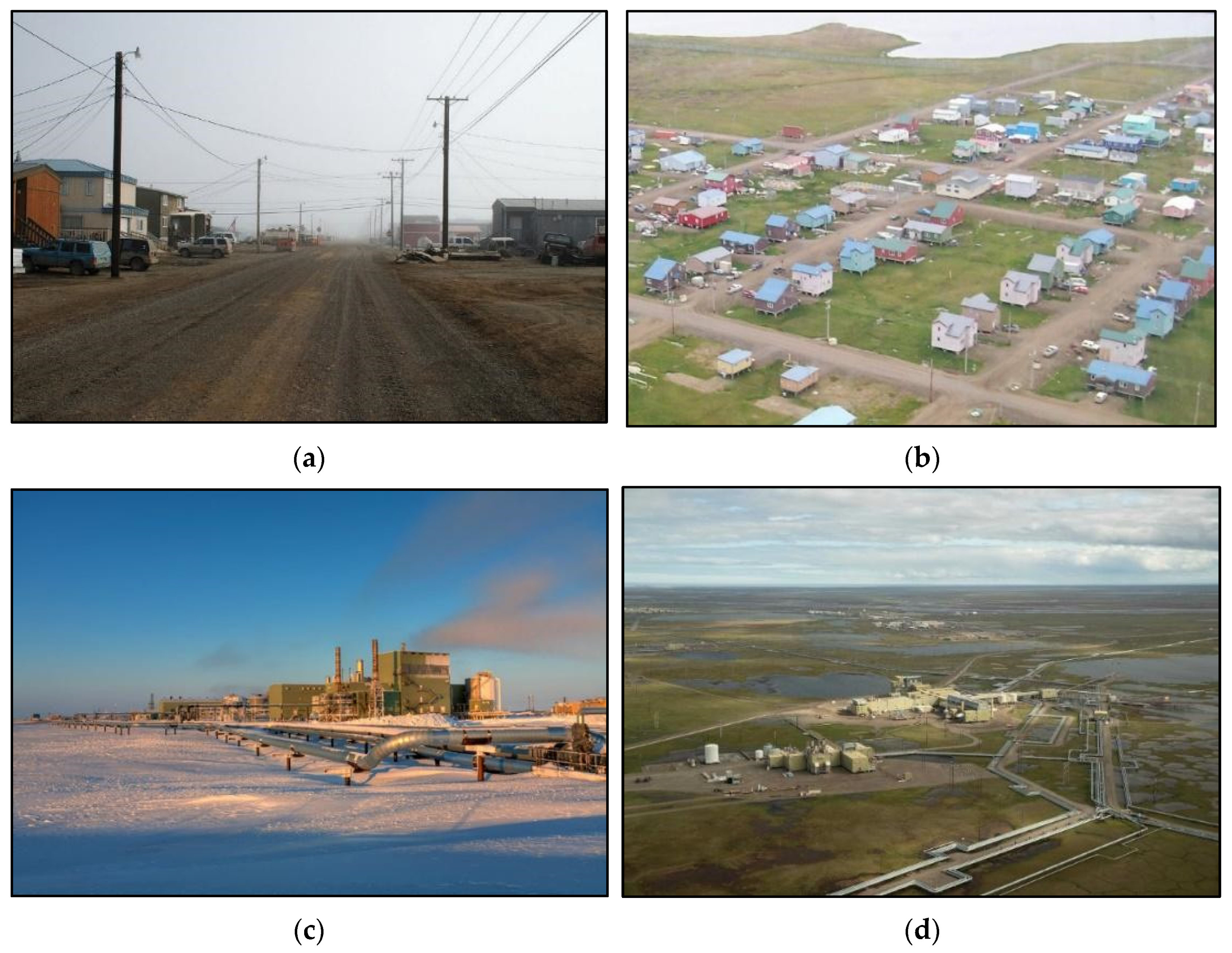
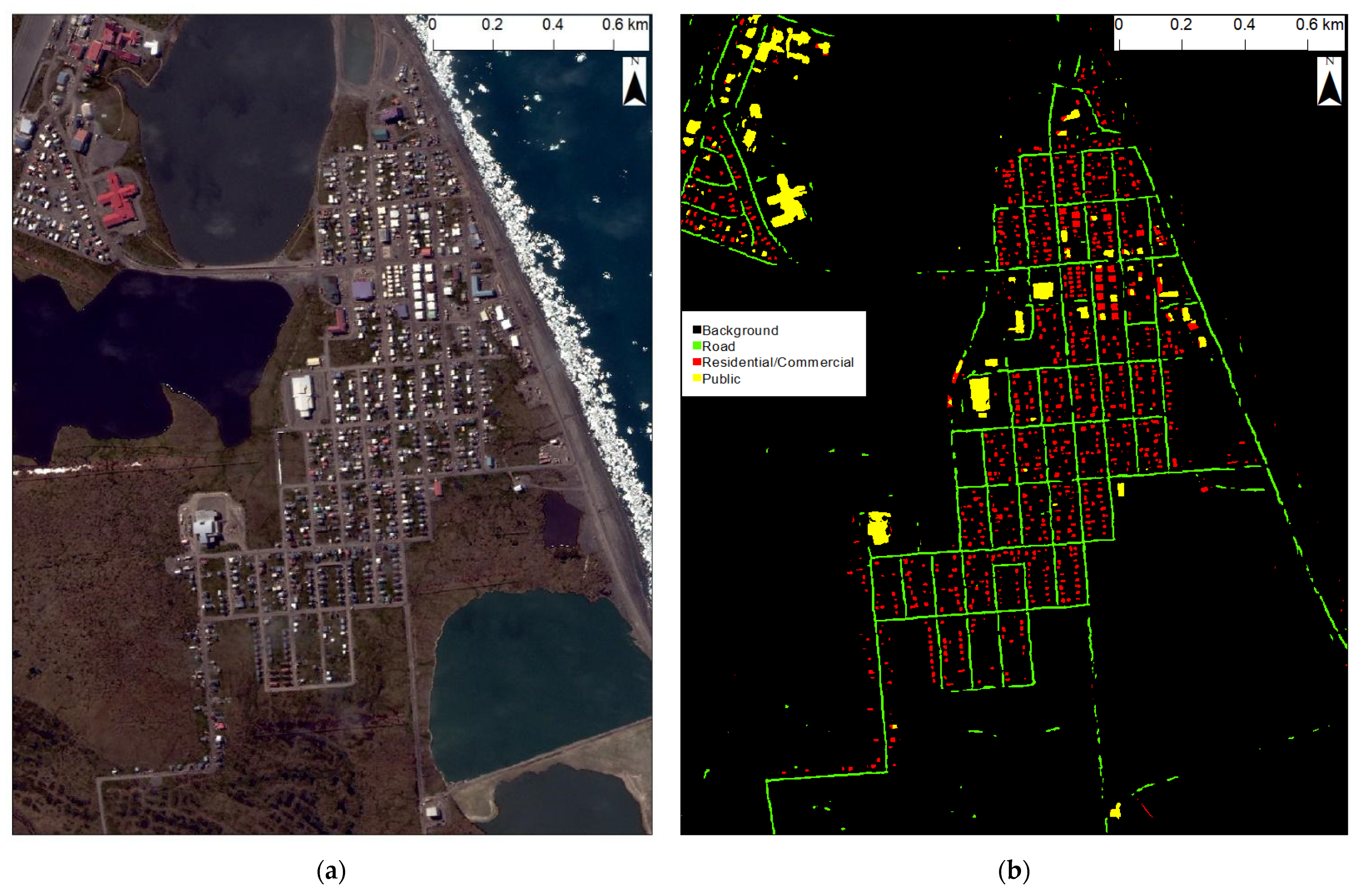
2.1. Study Area and Data

We selected two study sites on the North Slope of Alaska: (1) Utqiagvik and (2) Prudhoe Bay (Figure 1). Utqiagvik is the largest city of the North Slope Borough and the 12th-most populated city in Alaska; therefore, infrastructure is strongly developed there, with residential and commercial buildings, public buildings, pipelines, and roads (Figure 2a,b). Prudhoe Bay is one of the most prominent industrial areas in the Arctic [16]. The Prudhoe Bay oil field comprises an extensive network of infrastructure supporting the oil and gas extraction process, including multiple gathering centers, flow stations, pipelines, and roads connecting all facilities (Figure 2c,d). Therefore, Utqiagvik provided training samples for residential/commercial, public, and road infrastructure classes. Prudhoe Bay provided training samples for an industrial infrastructure class and added to the road class.

To train and test the U-Net CNN, we utilized six VHSR commercial satellite images in total from the WorldView-02 (WV-02) and QuickBird-02 (QB-02) sensors, two for the Utqiagvik site and four for the Prudhoe Bay site. We strictly utilized the blue, green, red, and near-infrared bands of the imagery. Specific details of the imagery used at each site, including acquisition date, sensor, and spatial resolution, are given in

Table 2. General characteristics of VHSR commercial satellite image scenes used to train and test the U-Net CNN.

Study Area	Sensor	Acquisition Date	Spatial Resolution (m)
Utqiagvik	WV-02	8 September 2014	0.72 × 0.87
	QB-02	1 August 2002	0.67 × 0.71
Prudhoe Bay	WV-02	7 September 2014	0.50 × 0.50
	WV-02	7 September 2014	0.50 × 0.50
	QB-02	21 August 2009	0.62 × 0.58
	QB-02	21 August 2009	0.62 × 0.60

. All of the images were provided by the Polar Geospatial Center at the University of Minnesota.

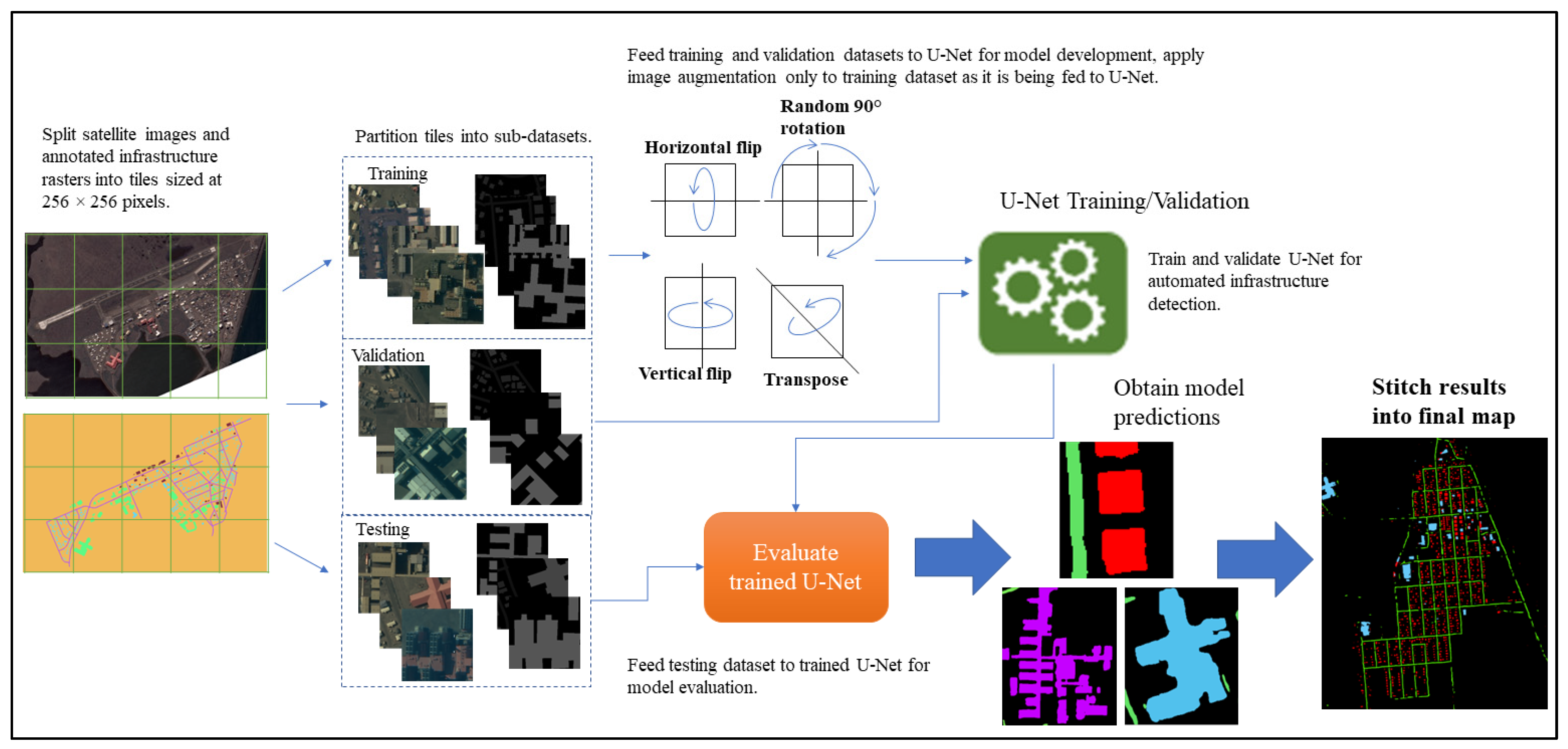
2.2. Generalized Workflow

Our workflow rests upon four stages: (1) input preparation, (2) model training and validation, (3) model evaluation, and (4) output postprocessing (Figure 3). Input preparation is based on two key operations. First, annotated infrastructure samples from each image were rasterized, and then satellite images and corresponding annotated raster layers for each site were split into smaller tiles sized at 256 pixels by 256 pixels. Second, these tile pairs (both images and masks) were randomly partitioned into sub-datasets for training, validation, and testing, utilizing an 80:10:10 split. Our training dataset consisted of 119 tile pairs, and both our validation and testing datasets consisted of 17 tile pairs (153 tile pairs in total). Once the input was prepared, we trained and validated the model, applying image augmentation techniques to the training dataset in order to synthetically inflate its size. Next, we evaluated the model’s performance on the testing dataset, which the model had not previously seen, and obtained accuracy metrics and model predictions. Finally, we performed postprocessing on the output by stitching the predicted tiles together into a final map.

2.3. Annotated Data Collection

In most remote sensing applications of a CNN, annotated data would need to be produced by drawing features of interest through an on-screen digitizing process. However, given that infrastructure of major settlements is consistently monitored by some governments, high-quality geospatial datasets are consistently maintained and can be utilized for CNN development if one can gain access to them. In the case of this study, we were able to obtain such a dataset. In addition, volunteered mapping efforts such as OpenStreetMap provide global coverage of buildings and roads in several areas of the Arctic. However, quality assessment must be performed to ensure locational accuracy before using OpenStreetMap in CNN training, given inconsistencies due to the nature of this kind of data.

Annotated data for the Utqiagvik study site comprised a geospatial vector dataset of building footprints (polygon features) and road centerlines (line features), which were digitized from 2019 aerial photography of the city by the North Slope Borough (NSB) GIS division. (This imagery belongs to the NSB and was not a part of our dataset, but the data layers extracted from the imagery were provided to us upon request). In the training data, we applied a buffer to road centerlines to convert them to polygons. The optimal buffer size was decided based on accurate overlapping between the polygon features representing the roads and the actual roads in the imagery. In the NSB dataset, features corresponding to a building footprint were classified as either a residential, commercial, public, or unoccupied building. We omitted unoccupied buildings and merged the residential and commercial classes together, as there were not enough commercial building features in the dataset to train the U-Net to detect this type of infrastructure. Manual editing of this data was conducted to ensure that polygon features corresponding to specific buildings and roads aligned with those structures in the satellite imagery, accounting for discrepancies between the aerial photography used for digitization and the satellite imagery used for the analysis. Furthermore, given the difference in acquisition dates of the aerial photography (2019) and the satellite imagery (2002, 2009, 2014), either certain digitized structures were not present in the satellite imagery, or structures present in the satellite imagery were not digitized. As a result, some features had to be removed from the dataset, and missing structures had to be digitized. Annotated data for the Prudhoe Bay study site comprised OpenStreetMap data that provided footprints of industrial structures and roads. Manual editing of this data was conducted to ensure that polygon features aligned with the industrial structures and roads in the satellite imagery.

The number of buildings and roads from each location that make up the dataset are described in

Table 3. Number of features (individual structures) belonging to each infrastructure type in the dataset.

	Residential/Commercial	Public	Industrial	Road
Utqiagvik	1243	88	n/a	223
Prudhoe Bay	n/a	n/a	102	30

. These samples are then rasterized, since CNNs require their input to be in the form of an image. After splitting the data into sub-datasets, we can measure the size of each target class as the number of pixels in the labeled masks belonging to each class, as seen in

Table 4. Class sizes in each sub-dataset measured as number of pixels in the labeled masks.

	Background	Residential/Commercial	Public	Industrial	Road
Training	6,528,038	352,686	155,131	525,418	237,511
Validation	883,507	71,180	33,795	54,917	70,713
Testing	809,311	52,387	30,600	177,327	44,487

.

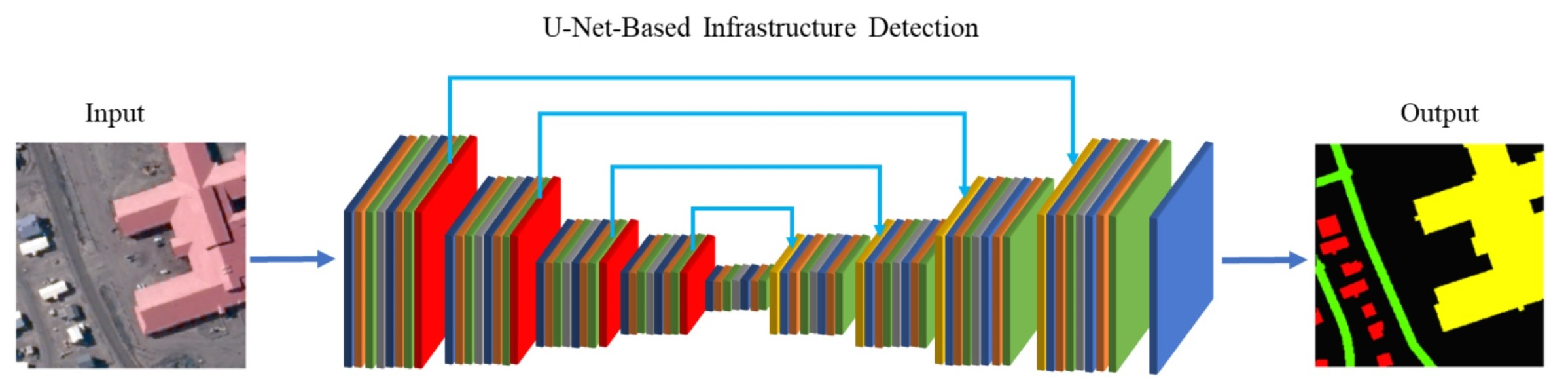
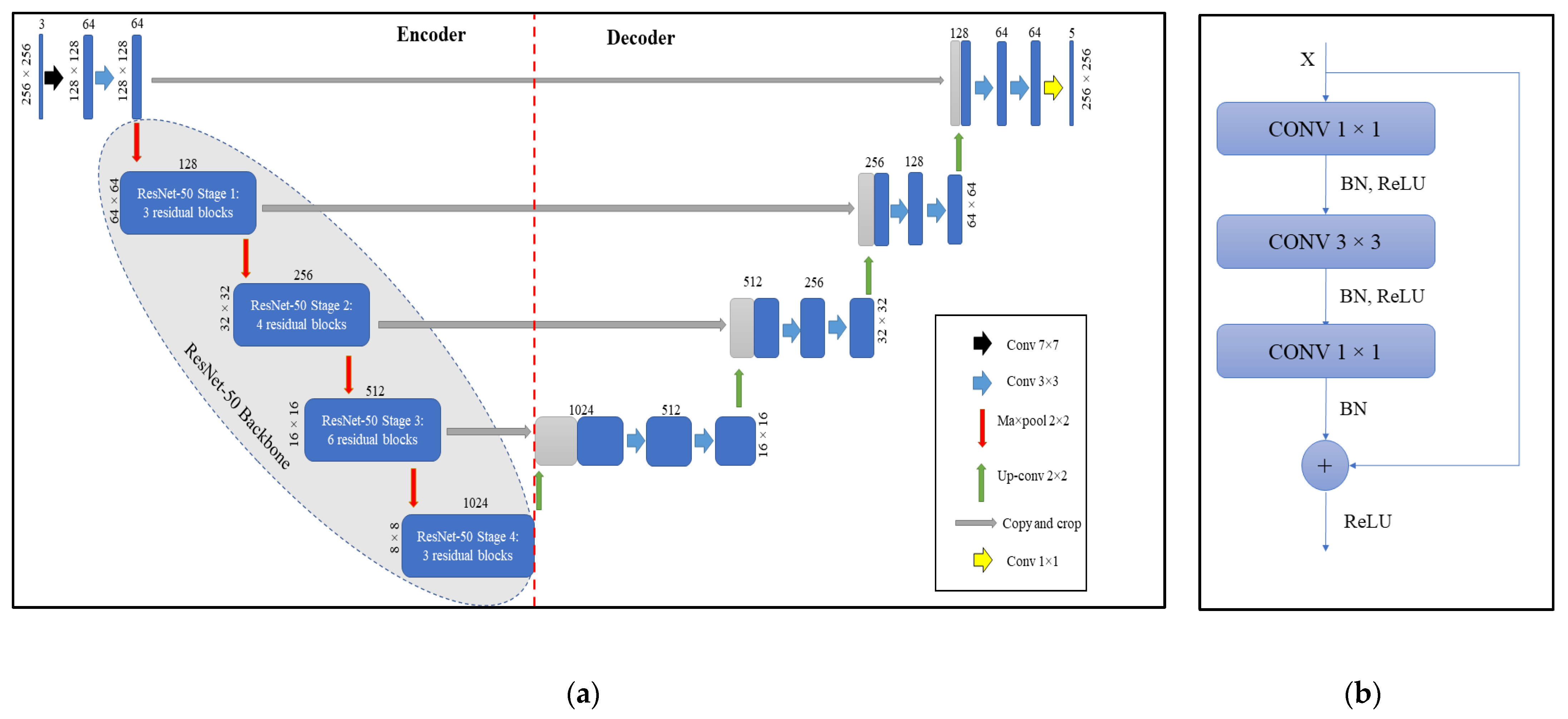
2.4. Deep Learning Algorithm

We chose to task a U-Net CNN with semantic segmentation of VHSR satellite imagery due to its success in various image analysis tasks and computational efficiency. The U-Net was first developed for biomedical image segmentation [37] and has since spread to a wide range of applications, such as remote sensing. The U-Net is a fully convolutional neural network defined by its U-shaped architecture, hence the name “U-Net,” that consists of an encoding and decoding path. The encoding path is also known as the analysis path or contracting path, and the decoding path is also known as the synthesis path or expansive path. The former shapes the typical CNN, consisting of repeated application of convolutions, each followed by a rectified linear unit (ReLU) and a max pooling operation. The function of the encoding path is to reduce the dimensionality of the input layers and increase the number of feature channels. In this route, a 3 × 3 convolution is followed by ReLU and 2 × 2 max pooling that downsamples and doubles the feature channels. On the other hand, the decoding path functions opposite to the encoding path. It reduces the number of channels and increases the spatial dimensions of the layers. The number of channels is halved in an upsampling process using 2 × 2 convolution at the start of the decoding route. Afterward, 3 × 3 convolution layers followed by ReLU are used. Skip connections are used to concatenate the corresponding feature layer from the encoding path to recover the information lost during downsampling in the encoding route. Finally, the dimension of the layers is restored using 1 × 1 convolution to generate a pixelwise classified predicted map.

However, in order to account for limited training data, we implemented transfer learning in order to leverage knowledge representations of low-level features (e.g., edges, lines, corners) learned by networks that have been pre-trained on large datasets for other computer vision tasks. We replaced the encoding path of the U-Net with a ResNet-50 backbone that was pre-trained on the ImageNet dataset. ResNet, or the residual neural network [38], is a CNN that utilizes identity skip connections to address the degradation problem that arises when accuracy gets saturated and degrades rapidly as network depth increases. It is constructed by stacking multiple bottleneck residual blocks, which consist of series of 1 × 1, 3 × 3, and 1 × 1 convolutions, as seen in Figure 4b. The backbone is frozen so as to avoid losing any of the information that its layers contain during training. Meanwhile, the U-Net decoder remains unfrozen and trainable in order to adjust to the parameters of the pre-trained layers. Figure 4a depicts the architecture of our U-Net model with a ResNet-50 backbone.

2.5. Model Training

The model was constructed and trained using PyTorch 1.10 and the Segmentation Models for PyTorch library (https://github.com/qubvel/segmentation_models.pytorch (accessed on 1 April 2021)), with a hardware configuration of an Intel Core i7-10750H 6-Core Processor and NVIDIA GeForce RTX 2060 with 6 GB of dedicated VRAM. Hyperparameters for model training are listed in

Table 5. Hyperparameters for model training.

Hyperparameter	Value/Type
Input size	256 × 256 pixels
Batch size	8
Epochs	60
Loss function	Dice Loss
Optimizer	Adam
Learning rate	0.001

.

To account for limited training data, we employed image augmentation to synthetically inflate the training data space through data warping, which generates additional samples through transformations applied in the dataspace [39]. We created copies of existing image tiles by applying four non-destructive geometric transformations that do not add to or detract from an image’s information: random 90° rotation, horizontal flip (reflection across horizontal axis), vertical flip (reflection across vertical axis), and transposition (reflection across either diagonal axis). Figure 5 provides a diagram visualizing these transformations. We conducted a systematic experiment to understand how these different transformations improve the performance of the U-Net and determine the optimal set of augmentations. The experiment consisted of six trials, in which we trained the model under different conditions: one trial for each of the selected transformations applied to the training dataset individually (four trials), one trial for all of the transformations applied together, and one trial for no image augmentation.

2.6. Accuracy Assessment

The accuracy of infrastructure detection performed by the model was assessed through standard semantic segmentation metrics: Recall, Precision, and F1 score. Recall represents the fraction of correctly labeled pixels of each class and is calculated as the ratio of positives identified by the model to the actual number of true positives:

$$Recall=\frac{True Positives}{True Positives+False Negatives}$$

(1)

Precision represents the fraction of detected pixels in each class that belong to the assigned class and is calculated as the ratio of true positives compared to all positives identified by the model:

$$Precision=\frac{True Positives}{True Positives+False Positives}$$

(2)

F1 score combines both recall and precision together to assess overall model performance:

$$F1=2\times \frac{Recall\times Precision}{Recall+Precision}$$

(3)

Recall, Precision, and F1 score were calculated for each target class. F1 score was averaged across all classes for an overall assessment of model performance. Furthermore, accuracy assessment was conducted for each trial of the augmentation experiment to determine the optimal augmentation method(s). Finally, we utilized the confusion matrix to visualize true and false positives and negatives for each class that the model was trained to detect.

3. Results

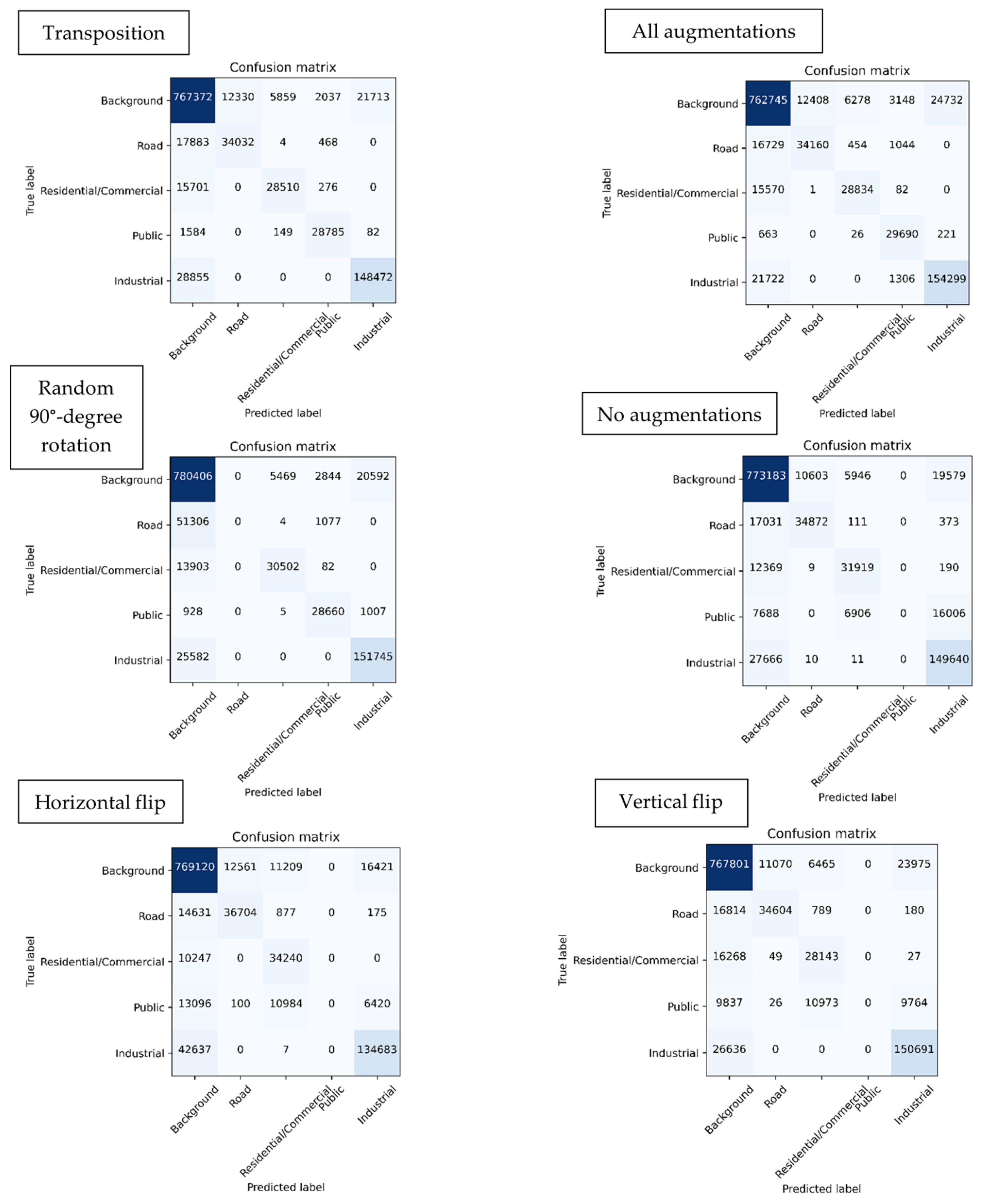
3.1. Quantitative Metrics

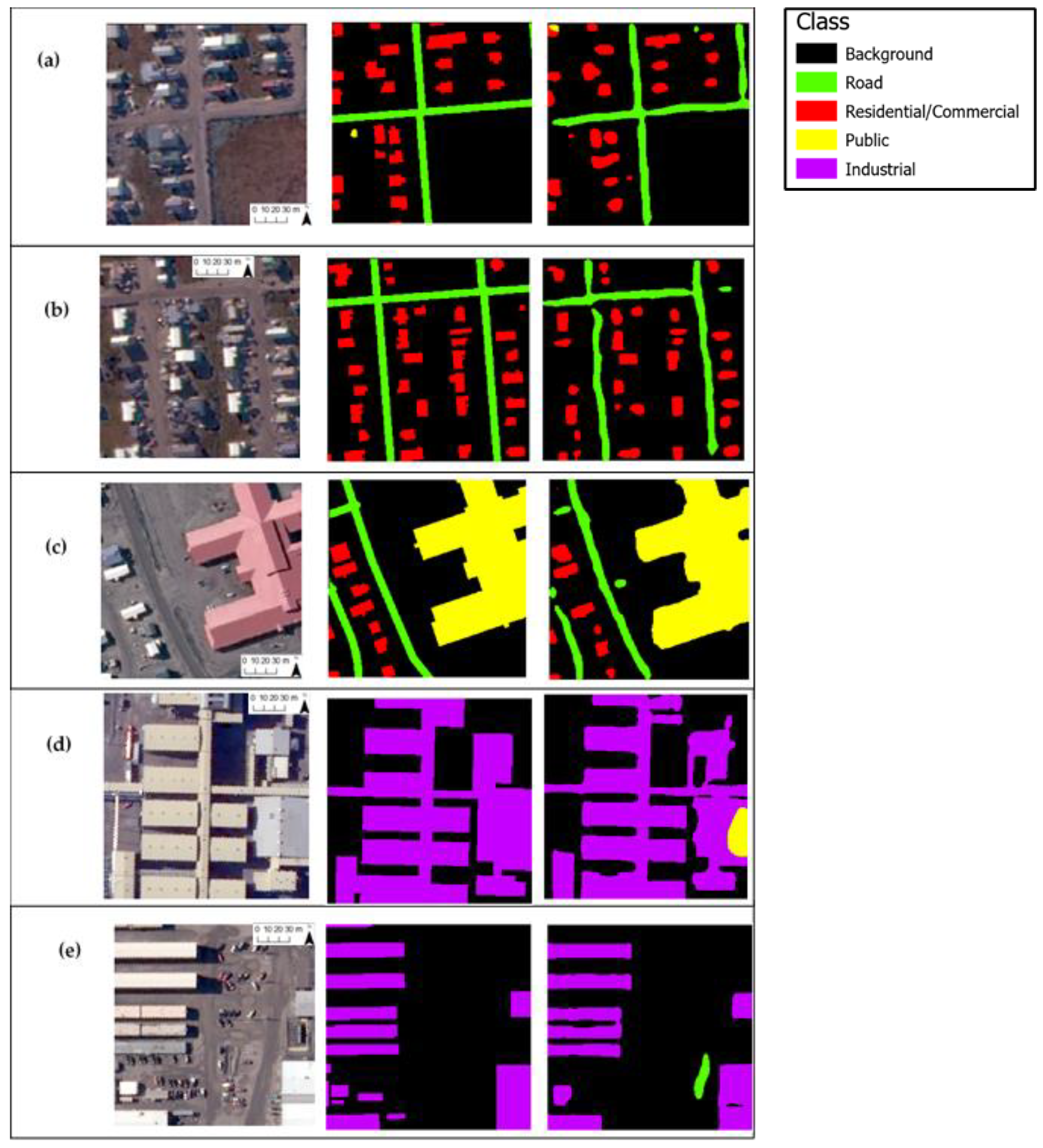
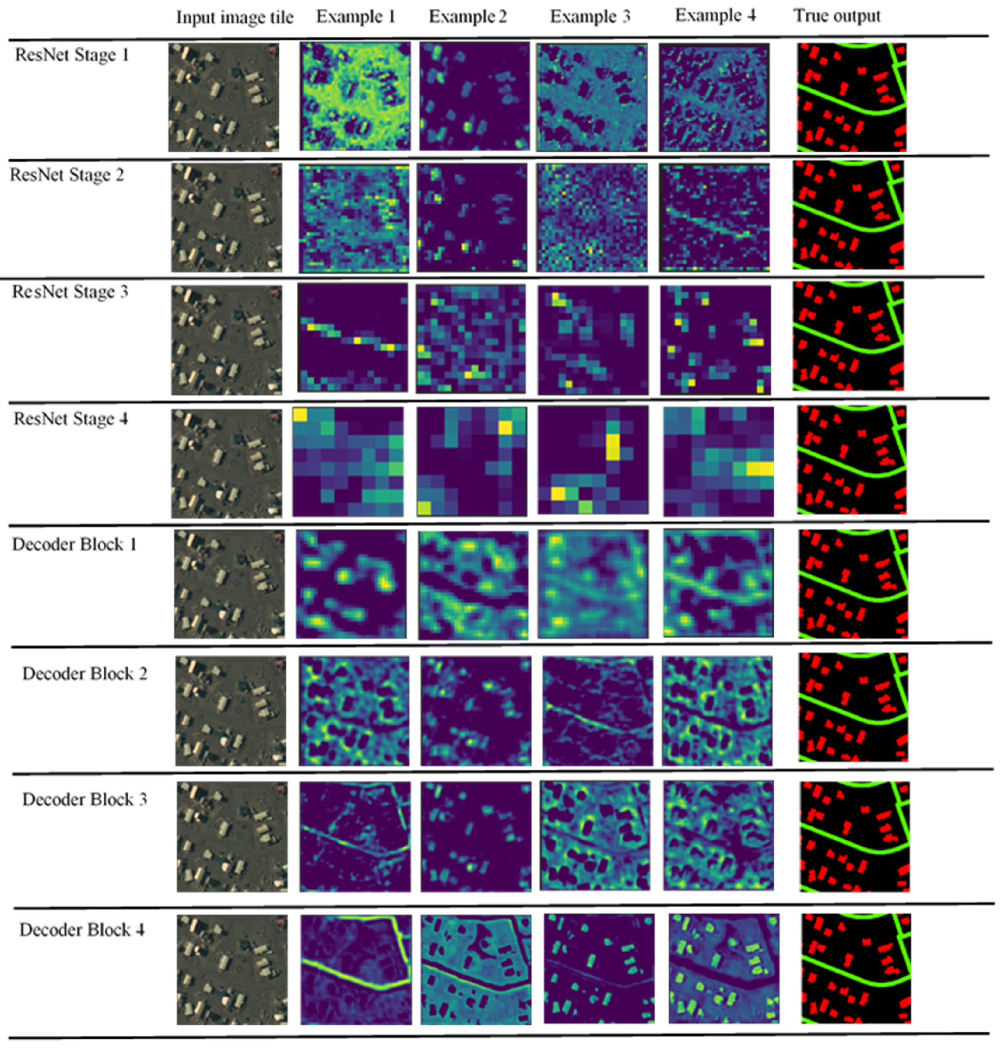
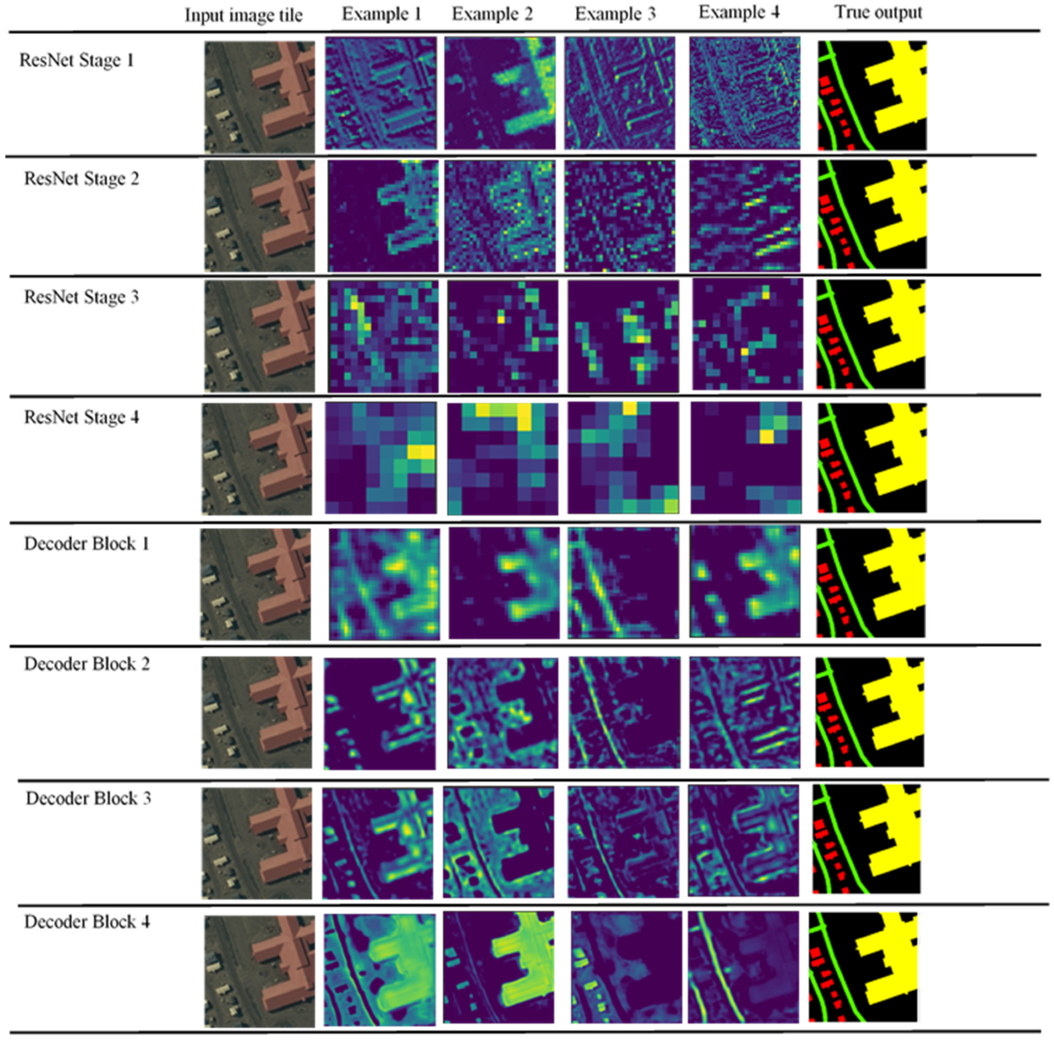
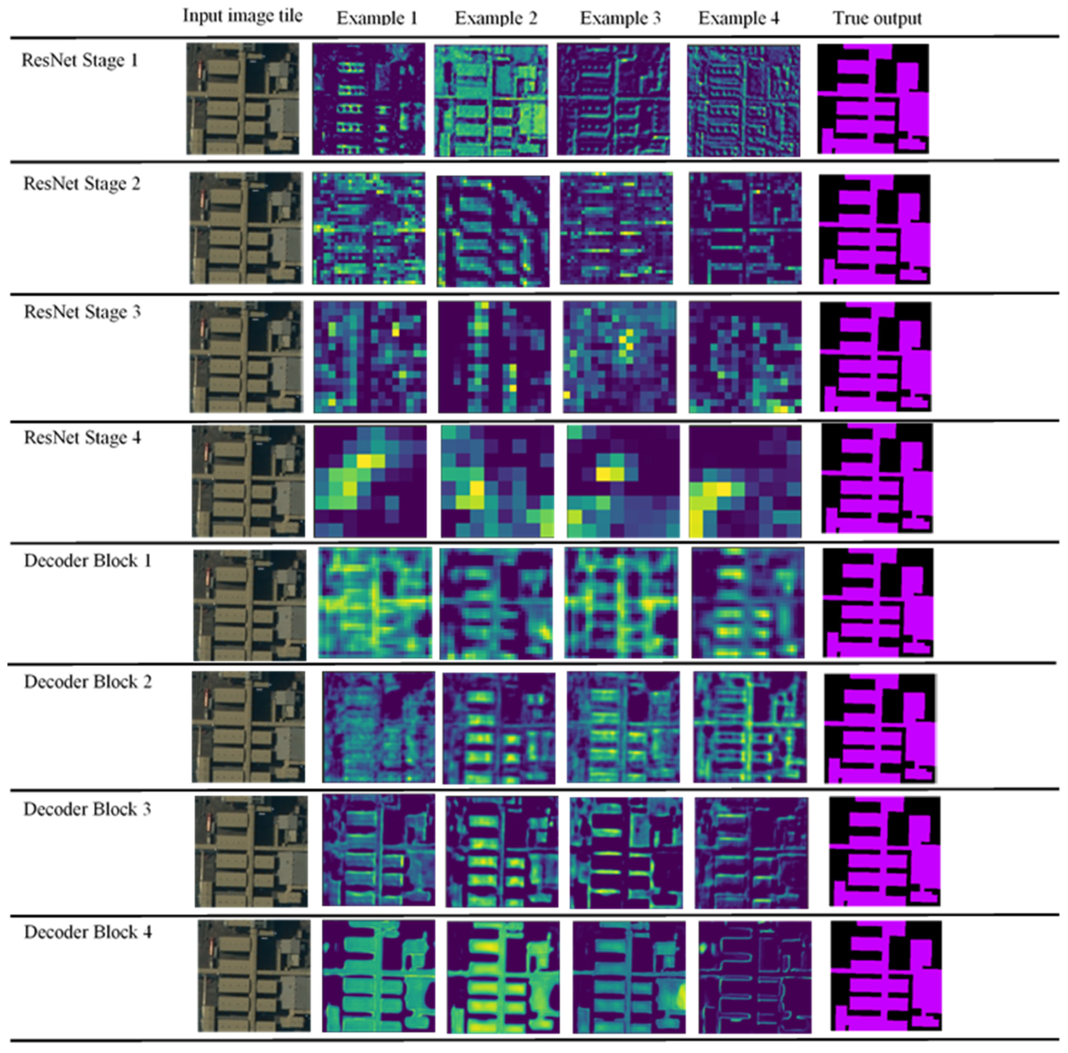
The results of model accuracy assessment and the augmentation experiment are displayed in

Table 6. Per-class accuracy metrics and average F1 score resulting from augmentation experiment. Table is organized by augmentation method in descending order of average F1 score.

Augmentation Method		Precision	Recall	F1-Score	Average F1-Score
Transposition	Background	0.92	0.95	0.94	0.83
	Road	0.73	0.65	0.69
	Residential/Commercial	0.83	0.64	0.72
	Public	0.91	0.94	0.93
	Industrial	0.87	0.84	0.85
All	Background	0.93	0.94	0.94	0.82
	Road	0.73	0.65	0.69
	Residential/Commercial	0.81	0.65	0.72
	Public	0.84	0.97	0.90
	Industrial	0.86	0.87	0.87
Random 90° rotation	Background	0.89	0.96	0.93	0.69
	Road	0.00	0.00	0.00
	Residential/Commercial	0.85	0.69	0.76
	Public	0.88	0.94	0.91
	Industrial	0.88	0.86	0.87
None	Background	0.92	0.96	0.94	0.64
	Road	0.77	0.67	0.71
	Residential/Commercial	0.71	0.72	0.71
	Public	0.00	0.00	0.00
	Industrial	0.81	0.84	0.82
Horizontal flip	Background	0.91	0.95	0.93	0.63
	Road	0.74	0.70	0.72
	Residential/Commercial	0.60	0.77	0.67
	Public	0.00	0.00	0.00
	Industrial	0.85	0.76	0.80
Vertical flip	Background	0.93	0.93	0.93	0.62
	Road	0.72	0.69	0.70
	Residential/Commercial	0.51	0.72	0.60
	Public	0.00	0.00	0.00
	Industrial	0.82	0.88	0.85

. Transposition and all augmentations applied together both yielded the highest model accuracy, with average F1 scores of 0.83 and 0.82, respectively. These two methods were considered to be the optimal augmentations, compared to the other four methods that yielded significantly lower scores. The next highest average F1 score came from the model trained on the dataset with random 90° rotation applied. This disparity between the top two scores and the bottom four scores can be attributed to the fact that either roads or public buildings were completely missed by the model in the bottom four trials. The residential/commercial and industrial classes were the most stable in terms of model detection. This may be attributed to the fact that they were better represented in the training data compared to the public and road classes (Table 4). Furthermore, roads at both study sites are largely unpaved and narrow, making it difficult for the model to detect roads as features separate from the background. However, as shown, optimal image augmentation methods can aid performance when training data is lacking.

Confusion matrices showing the number of correctly and incorrectly classified pixels for each infrastructure class and augmentation trial are available in Figure 6 and corroborate Table 6. These are a useful tool for visualizing the true and false positives and negatives used to calculate the reported accuracy metrics, as well as understanding how the model confuses classes during detection. It can be seen that there are varying sources of false positives and negatives. In the two highest-scoring model trials (transposition and all augmentations), confusion between infrastructure classes is largely reduced, and the only significant source of confusion is misclassification of infrastructure as background and vice versa. However, when less effective augmentation methods, or no augmentation, are applied, infrastructure classes are confused for each other at significantly higher rates. For example, public buildings are largely confused for residential/commercial and industrial buildings when either horizontal/vertical flipping or no augmentations are applied. Furthermore, the most notable difference in model confusion between the optimal and less optimal augmentations is that no infrastructure classes were missed when the optimal augmentations were applied, as seen in Table 6.

3.2. Visual Results

In addition to quantitative evaluation, visual results are shown in Figure 7, Figure 8, Figure 9, Figure 10 and Figure 11, which were produced using the model with the highest average F1 score. Selected model predictions on input tiles from the test dataset are shown in Figure 7, with each infrastructure class and both Utqiagvik and Prudhoe Bay study sites being shown. A final map of predicted infrastructure in Utqiagvik is shown in Figure 8.

Figure 9, Figure 10 and Figure 11 show convolutional feature maps (CFMs) extracted during training from the final activation function of each major stage of the model, as shown in Figure 4. A CFM is the output of a convolution operation between a given filter (or kernel) and input image (or output of a previous layer), and it is computed as the dot product of these two during a sliding-window operation. Individual CFMs visualize the features that a CNN is learning at a particular stage in the network. Viewing all the CFMs together from an entire training process reveals the complete feature representation with multi-level abstraction that a network has constructed for target features. In the U-Net encoder, convolutional filters detect increasingly more abstract features, or low-level features, that are propagated to the decoder, which constructs these into higher level features and eventually an output segmentation map. Four CFMs are selected from each stage of the encoder and decoder, serving as examples of the feature representations that the model constructs for each infrastructure class. Ultimately, CFMs prove to be a useful diagnostic, as they allow researchers to internally assess the learning process at each stage and visually identify where detection fails or succeeds.

4. Discussion

In this paper, we presented the first exploratory study of automated Arctic built infrastructure detection from VHSR satellite imagery using a CNN. Only one previous study [22] has successfully demonstrated automated detection of infrastructure with machine learning and deep learning on the pan-Arctic scale, while others relied on manual digitization or semi-automated analysis at local scales. This study served as an initial assessment of CNN-based automated detection from VHSR satellite imagery by testing the methodology on two Alaskan North Slope locations and five common infrastructure types. Overall, model accuracy assessment shows that the U-Net CNN with a transfer learning approach can successfully automate detection of various infrastructure types with high segmentation accuracy. Buildings for residential and commercial use, public use, and industrial use, as well as roads, can all be detected and delineated as individual features (Figure 7 and Figure 8).

We conducted an image augmentation experiment to specifically address the challenge of limited training data that hampers most CNN-based detection tasks. Results show that optimal augmentation methods can reduce inter-class confusion among infrastructure types and improve the overall F1 score from a minimum of 0.62 to a maximum of 0.83 (Table 5). However, augmentation yielded virtually no improvement in the recall of the residential/commercial and road classes, which was 0.65 for both of these classes when all augmentation methods were applied. This indicates that the model still misses a large portion of residential/commercial buildings and roads, either by completely failing to detect a structure or not detecting the full extent of a structure. Ultimately, this implies that there is a limit on the amount of synthetic inflation that image augmentation can induce in small training datasets. Therefore, we expect to see improved performance in these classes as we collect or produce more training samples. We recognize this to be the most important scope of improvement for this work, as CNNs are “data-hungry” models and can be drastically improved by training with more samples.

Furthermore, expanding the training dataset includes expanding the geographic extent of automated infrastructure detection by sampling different communities and industrial locations across the Alaskan North Slope and the broader pan-Arctic region. This will allow us to assess the transferability of CNN-based automated infrastructure detection, which is a significant step in developing our methodology because infrastructure and its landscape context can vary widely across the Arctic. For example, infrastructure across different settlements can vary in terms of size, shape, building material, density of surrounding infrastructure, and more. In addition, landscape backgrounds differ across Arctic regions, resulting in variability of contextual information that a CNN would need to recognize in order to properly detect infrastructure. If the training data is unable to capture this inherent variability, the operational utility of the CNN will be severely limited. Therefore, systematic experimentation is required in order to understand the transferability mechanism.

Expanding the training dataset can also include enhancing the thematic depth of the model to discern other infrastructure classes. As mentioned, in this study we focused on roads and different building types, but there are several characteristic infrastructure types that define the Arctic built environment which we have not addressed. These include impervious cover, gravel pads, and fuel and water pipelines, all of which are essential structures for studying and understanding the interlinkages between permafrost disturbance and infrastructure in expanding industrial areas. Of particular relevance in Arctic permafrost regions is piping infrastructure, which is largely constructed above ground because it is easier to maintain when permafrost thaws and also reduces the risk of disturbing permafrost. This makes remote sensing especially relevant in monitoring Arctic infrastructure. However, experimentation in this aspect is necessary, given that as the number of classes increases, the learning process for a CNN becomes more complex and may lead to higher inter-class confusion, especially between linear features like roads and pipelines that may appear similar in satellite imagery.

Finally, as these points of improvement are addressed and the automated built infrastructure detection workflow is refined, we will have the opportunity to incorporate it with existing optimized automated detection workflows, such as the Mapping Application for Arctic Permafrost Land Environment (MAPLE) [40,41]. MAPLE has successfully produced the first pan-Arctic ice-wedge polygon map, with over 1 billion individual ice-wedge polygons detected and classified, including mapped surface water as well. MAPLE is also being expanded to automatic detection of ice-wedge troughs. As ice-wedge polygon type (low-centered or high-centered) and growth of troughs can indicate permafrost degradation, combining built infrastructure maps with ice-wedge polygon, ice-wedge trough, and water maps can be used to identify areas where infrastructure is susceptible to the damaging effects of permafrost thawing.

5. Conclusions

Imagery-based infrastructure mapping of Arctic permafrost landscapes has been constrained to human-augmented workflows, namely manual digitization and semi-automated workflows, on locally confined scales. Only one study has successfully automated mapping on the pan-Artic scale but is limited to the use of 10 m Sentinel-1 and Sentinel-2 imagery within a 100 km distance of the Arctic coast. The rapid influx of sub-meter spatial resolution commercial satellite imagery into the Arctic science community provides the opportunity to map infrastructure across the entire Arctic at a fine scale (<1 m). However, image analysis workflows required for this task have not been developed or tested. In this study, we applied the U-Net with a Res-Net 50 backbone, combined with image augmentation, to automatically detect different infrastructure types in two Alaskan North Slope locations (industrial Prudhoe Bay and the City of Utqiagvik). Our results show that with limited training data, the U-Net can achieve an average F1 score of 0.83 in multi-class semantic segmentation of VHSR satellite imagery for automated infrastructure detection when optimal augmentation methods are applied.

While the U-Net shows promising ability in automatically detecting Arctic built infrastructure, further studies are necessary to advance the geographic and thematic domain of the workflow and fully understand its abilities in these avenues. Therefore, our future work can focus on two main directions revolving around expansion of the training dataset: (1) systematic experimentation on the transferability of the U-Net across Arctic locations; (2) enhancing the thematic depth of the U-Net by adding more infrastructure classes to the training dataset.

References

1. Brown, J.; Ferrians, O.J., Jr.; Heginbottom, J.A.; Melnikov, E.S. Circum-Arctic Map of Permafrost and Ground-Ice Conditions; National Snow and Ice Data Center: Boulder, CO, USA, 1997; Available online: https://nsidc.org/data/ggd318 (accessed on 10 February 2022).
2. Biskaborn, B.K.; Smith, S.L.; Noetzli, J.; Matthes, H.; Vieira, G.; Streletskiy, D.A.; Schoeneich, P.; Romanovsky, V.E.; Lewkowicz, A.G.; Abramov, A.; et al. Permafrost is warming at a global scale. Nat. Commun. 2019, 10, 264. [Google Scholar] [CrossRef] [PubMed] [Green Version]
3. Comiso, J.C.; Hall, D.K. Climate trends in the Arctic as observed from space. WIREs Clim. Chang. 2014, 5, 389–409. [Google Scholar] [CrossRef]
4. Kokelj, S.V.; Jorgenson, M.T. Advances in Thermokarst Research. Permafr. Periglac. Process. 2013, 24, 108–119. [Google Scholar] [CrossRef]
5. Hjort, J.; Karjalainen, O.; Aalto, J.; Westermann, S.; Romanovsky, V.E.; Nelson, F.E.; Etzelmüller, B.; Luoto, M. Degrading permafrost puts Arctic infrastructure at risk by mid-century. Nat. Commun. 2018, 9, 1–9. [Google Scholar] [CrossRef]
6. Nelson, F.E.; Anisimov, O.A.; Shiklomanov, N.I. Subsidence risk from thawing permafrost. Nature 2001, 410, 889–890. [Google Scholar] [CrossRef] [PubMed]
7. Melvin, A.M.; Larsen, P.; Boehlert, B.; Neumann, J.E.; Chinowsky, P.; Espinet, X.; Martinich, J.; Baumann, M.S.; Rennels, L.; Bothner, A.; et al. Climate change damages to Alaska public infrastructure and the economics of proactive adaptation. Proc. Natl. Acad. Sci. USA 2016, 114, E122–E131. [Google Scholar] [CrossRef] [Green Version]
8. Streletskiy, D.A.; Suter, L.J.; Shiklomanov, N.I.; Porfiriev, B.N.; Eliseev, D.O. Assessment of climate change impacts on buildings, structures and infrastructure in the Russian regions on permafrost. Environ. Res. Lett. 2019, 14, 025003. [Google Scholar] [CrossRef]
9. Suter, L.; Streletskiy, D.; Shiklomanov, N. Assessment of the cost of climate change impacts on critical infrastructure in the circumpolar Arctic. Polar Geogr. 2019, 42, 267–286. [Google Scholar] [CrossRef]
10. Ramage, J.; Jungsberg, L.; Wang, S.; Westermann, S.; Lantuit, H.; Heleniak, T. Population living on permafrost in the Arctic. Popul. Environ. 2021, 43, 22–38. [Google Scholar] [CrossRef]
11. Barros, V.R.; Field, C.B.; Dokken, D.J.; Mastrandrea, M.D.; Mach, K.J.; Bilir, T.E.; Chatterjee, M.; Ebi, K.L.; Estrada, Y.O.; Genova, R.C.; et al. Climate Change 2014: Impacts, Adaptation, and Vulnerability. Part B: Regional Aspects. Contribution of Working Group II to the Fifth Assessment Report of the Intergovernmental Panel on Climate Change; Cambridge University Press: Cambridge, UK; New York, NY, USA, 2014; Available online: https://www.ipcc.ch/site/assets/uploads/2018/02/WGIIAR5-PartB_FINAL.pdf (accessed on 10 February 2022).
12. Larsen, P.; Goldsmith, S.; Smith, O.; Wilson, M.; Strzepek, K.; Chinowsky, P.; Saylor, B. Estimating future costs for Alaska public infrastructure at risk from climate change. Glob. Environ. Chang. 2008, 18, 442–457. [Google Scholar] [CrossRef]
13. Gautier, D.L.; Bird, K.J.; Charpentier, R.R.; Grantz, A.; Houseknecht, D.W.; Klett, T.R.; Moore, T.E.; Pitman, J.K.; Schenk, C.J.; Schuenemeyer, J.H.; et al. Assessment of Undiscovered Oil and Gas in the Arctic. Science 2009, 324, 1175–1179. [Google Scholar] [CrossRef] [PubMed] [Green Version]
14. Larsen, J.N.; Fondahl, G. Arctic Human Development Report—Regional Processes and Global Linkages; Nordic Council of Ministers: Copenhagen, Denmark, 2015. [Google Scholar] [CrossRef] [Green Version]
15. Anisimov, O.A.; Vaughan, D.G. Polar Regions (Arctic and Antarctic). Climate Change 2007: Impacts, Adaptation, and Vulnerability. Contribution of Working Group II to the Fourth Assessment Report of the Intergovernmental Panel on Climate Change; Cambridge University Press: Cambridge, UK, 2007; pp. 653–685. Available online: https://www.ipcc.ch/site/assets/uploads/2018/02/ar4-wg2-chapter15-1.pdf (accessed on 10 February 2022).
16. Raynolds, M.K.; Walker, D.A.; Ambrosius, K.J.; Brown, J.; Everett, K.R.; Kanevskiy, M.; Kofinas, G.P.; Romanovsky, V.E.; Shur, Y.; Webber, P.J. Cumulative geoecological effects of 62 years of infrastructure and climate change in ice-rich permafrost landscapes, Prudhoe Bay Oilfield, Alaska. Glob. Chang. Biol. 2014, 20, 1211–1224. [Google Scholar] [CrossRef]
17. Kanevskiy, M.; Shur, Y.; Walker, D.; Jorgenson, T.; Raynolds, M.K.; Peirce, J.L.; Jones, B.M.; Buchhorn, M.; Matyshak, G.; Bergstedt, H.; et al. The shifting mosaic of ice-wedge degradation and stabilization in response to infrastructure and climate change, Prudhoe Bay Oilfield, Alaska. Arct. Sci. 2022, 8, 498–530. [Google Scholar] [CrossRef]
18. Walker, D.A.; Raynolds, M.K.; Kanevskiy, M.Z.; Shur, Y.S.; Romanovsky, V.E.; Jones, B.M.; Buchhorn, M.; Jorgenson, M.T.; Šibík, J.; Breen, A.L.; et al. Cumulative impacts of a gravel road and climate change in an ice-wedge polygon landscape, Prudhoe Bay, AK. Arct. Sci. 2022. [Google Scholar] [CrossRef]
19. Arctic Monitoring and Assessment Programme (AMAP). Snow, Water, Ice and Permafrost in the Arctic (SWIPA), Oslo, Norway. 2017. Available online: https://www.amap.no/documents/doc/snow-water-ice-and-permafrost-in-the-arctic-swipa-2017/1610 (accessed on 11 February 2022).
20. Brown de Colstoun, E.C.; Huang, C.; Wang, P.; Tilton, J.C.; Tan, B.; Phillips, J.; Niemczura, S.; Ling, P.-Y.; Wolfe, R.E. Global Man-Made Impervious Surface (GMIS) Dataset from Landsat; NASA Socioeconomic Data and Applications Center (SEDAC): Palisades, NY, USA, 2017; Available online: https://sedac.ciesin.columbia.edu/data/set/ulandsat-gmis-v1/data-download (accessed on 11 February 2022).
21. Wang, P.; Huang, C.; Brown de Colstoun, E.; Tilton, J.; Tan, B. Global Human Built-Up and Settlement Extent (HBASE) Dataset from Landsat; NASA Socioeconomic Data and Applications Center (SEDAC): Palisades, NY, USA, 2017; Available online: https://sedac.ciesin.columbia.edu/data/set/ulandsat-hbase-v1/data-download (accessed on 11 February 2022).
22. Bartsch, A.; Pointner, G.; Ingeman-Nielsen, T.; Lu, W. Towards Circumpolar Mapping of Arctic Settlements and Infrastructure Based on Sentinel-1 and Sentinel-2. Remote Sens. 2020, 12, 2368. [Google Scholar] [CrossRef]
23. Kumpula, T.; Forbes, B.C.; Stammler, F.; Meschtyb, N. Dynamics of a Coupled System: Multi-Resolution Remote Sensing in Assessing Social-Ecological Responses during 2.5 Years of Gas Field Development in Arctic Russia. Remote Sens. 2012, 4, 1046–1068. [Google Scholar] [CrossRef] [Green Version]
24. Kumpula, T.; Forbes, B.; Stammler, F. Combining data from satellite images and reindeer herders in arctic petroleum development: The case of Yamal, West Siberia. Nord. Geogr. Publ. 2006, 35, 17–30. Available online: https://www.geobotany.uaf.edu/library/pubs/KumpulaT2006_nordGP_25_17.pdf (accessed on 12 February 2022).
25. Kumpula, T.; Forbes, B.; Stammler, F. Remote Sensing and Local Knowledge of Hydrocarbon Exploitation: The Case of Bovanenkovo, Yamal Peninsula, West Siberia, Russia. ARCTIC 2010, 63, 165–178. [Google Scholar] [CrossRef]
26. Kumpula, T.; Pajunen, A.; Kaarlejärvi, E.; Forbes, B.C.; Stammler, F. Land use and land cover change in Arctic Russia: Ecological and social implications of industrial development. Glob. Environ. Chang. 2011, 21, 550–562. [Google Scholar] [CrossRef]
27. Gadal, S.; Ouerghemmi, W. Multi-Level Morphometric Characterization of Built-up Areas and Change Detection in Siberian Sub-Arctic Urban Area: Yakutsk. ISPRS Int. J. Geo-Inf. 2019, 8, 129. [Google Scholar] [CrossRef] [Green Version]
28. Ourng, C.; Vaguet, Y.; Derkacheva, A. Spatio-temporal urban growth pattern in the arctic: A case study in surgut, Russia. In Proceedings of the 2019 Joint Urban Remote Sensing Event (JURSE), Vannes, France, 22–24 May 2019; pp. 1–4. [Google Scholar] [CrossRef]
29. Ardelean, F.; Onaca, A.; Chețan, M.-A.; Dornik, A.; Georgievski, G.; Hagemann, S.; Timofte, F.; Berzescu, O. Assessment of Spatio-Temporal Landscape Changes from VHR Images in Three Different Permafrost Areas in the Western Russian Arctic. Remote Sens. 2020, 12, 3999. [Google Scholar] [CrossRef]
30. Blaschke, T. Object based image analysis for remote sensing. ISPRS J. Photogramm. Remote Sens. 2010, 65, 2–16. [Google Scholar] [CrossRef] [Green Version]
31. Blaschke, T.; Hay, G.J.; Kelly, M.; Lang, S.; Hofmann, P.; Addink, E.; Feitosa, R.Q.; van der Meer, F.; van der Werff, H.; van Coillie, F.; et al. Geographic Object-Based Image Analysis—Towards a New Paradigm. ISPRS J. Photogramm. Remote Sens. 2014, 87, 180–191. [Google Scholar] [CrossRef] [Green Version]
32. He, K.; Gkioxari, G.; Dollár, P.; Girshick, R. Mask R-CNN. arXiv 2018, arXiv:1703.06870. [Google Scholar] [CrossRef]
33. Tiede, D.; Schwendemann, G.; Alobaidi, A.; Wendt, L.; Lang, S. Mask R-CNN-based building extraction from VHR satellite data in operational humanitarian action: An example related to COVID-19 response in Khartoum, Sudan. Trans. GIS 2021, 25, 1213–1227. [Google Scholar] [CrossRef] [PubMed]
34. Wang, Y.; Li, S.; Teng, F.; Lin, Y.; Wang, M.; Cai, H. Improved Mask R-CNN for Rural Building Roof Type Recognition from UAV High-Resolution Images: A Case Study in Hunan Province, China. Remote Sens. 2022, 14, 265. [Google Scholar] [CrossRef]
35. Li, W.; He, C.; Fang, J.; Zheng, J.; Fu, H.; Yu, L. Semantic Segmentation-Based Building Footprint Extraction Using Very High-Resolution Satellite Images and Multi-Source GIS Data. Remote Sens. 2019, 11, 403. [Google Scholar] [CrossRef] [Green Version]
36. Yang, M.; Yuan, Y.; Liu, G. SDUNet: Road extraction via spatial enhanced and densely connected UNet. Pattern Recognit. 2022, 126, 108549. [Google Scholar] [CrossRef]
37. Ronneberger, O.; Fischer, P.; Brox, T. U-Net: Convolutional networks for biomedical image segmentation. In Medical Image Computing and Computer-Assisted Intervention 2015; Navab, N., Hornegger, J., Wells, W.M., Frangi, A.F., Eds.; Springer International Publishing: Cham, Switzerland, 2015; pp. 234–241. [Google Scholar] [CrossRef] [Green Version]
38. He, K.; Zhang, X.; Ren, S.; Sun, J. Deep residual learning for image recognition. In Proceedings of the 2016 IEEE Conference on Computer Vision and Pattern Recognition (CVPR), Las Vegas, NV, USA, 27–30 June 2016; pp. 770–778. [Google Scholar] [CrossRef] [Green Version]
39. Wong, S.C.; Gatt, A.; Stamatescu, V.; McDonnell, M.D. Understanding data augmentation for classification: When to warp? In Proceedings of the International Conference on Digital Image Computing: Techniques and Applications (DICTA), Gold Coast, Australia, 30 November–2 December 2016; pp. 1–6. [Google Scholar] [CrossRef] [Green Version]
40. Udawalpola, M.; Hasan, A.; Liljedahl, A.K.; Soliman, A.; Witharana, C. Operational-Scale GeoAI for Pan-Arctic Permafrost Feature Detection from High-Resolution Satellite Imagery. Int. Arch. Photogramm. Remote Sens. Spat. Inf. Sci. 2021, XLIV-M-3-2, 175–180. [Google Scholar] [CrossRef]
41. Udawalpola, M.R.; Hasan, A.; Liljedahl, A.; Soliman, A.; Terstriep, J.; Witharana, C. An Optimal GeoAI Workflow for Pan-Arctic Permafrost Feature Detection from High-Resolution Satellite Imagery. Photogramm. Eng. Remote Sens. 2022, 88, 181–188. [Google Scholar] [CrossRef]
Figure 1. (a) Inset map showing both study sites within the extent of the Arctic, with red boxes indicating each site. (b,c) depict the Utqiagvik and Prudhoe Bay study sites, respectively, and the satellite images (natural color composite) used to train and test the U-Net CNN. Annotated areas are outlined by red boxes. Imagery © DigitalGlobe, Inc.
Remotesensing 14 02719 g001
Figure 2. (a) Unpaved road in Utqiagvik surrounded by residential buildings (photo credits: Andrei Taranchenko). (b) Residential neighborhood in Utqiagvik (photo credits: Native Village of Utqiagvik). (c) Gathering Center 1 on Prudhoe Bay oil field (photo credits: Lucas Payne). (d) Flow Station 1 on Prudhoe Bay oil field (photo credits: Judy Patrick).
Remotesensing 14 02719 g002
Figure 3. Diagram of generalized automated detection workflow. Imagery © DigitalGlobe, Inc.
Remotesensing 14 02719 g003
Figure 4. (a) Architecture of U-Net with ResNet-50 backbone. (b) Diagram of bottleneck residual block in ResNet-50.
Remotesensing 14 02719 g004
Figure 5. Diagram of selected geometric transformations. “M1 reflection” and “M3 reflection” refer to horizontal and vertical flipping, respectively. “M2 reflection” and “M4 reflection” refer to transposition.
Remotesensing 14 02719 g005
Figure 6. Confusion matrices from each model trained under the augmentation experiment. The matrices, starting from top left to bottom right, are ordered from left to right by the average F1 score achieved by the corresponding model. Horizontal axis indicates the pixel class predicted by the model, and vertical axis indicates the true pixel class. Number in each cell of the matrix indicates number of pixels.
Remotesensing 14 02719 g006
Figure 7. Selected model predictions on the testing dataset from the Utqiagvik and Prudhoe Bay sites. (a–e) each contain the input image tile, annotated image tile showing true output, and output predicted by the model from left to right. Imagery © DigitalGlobe, Inc.
Remotesensing 14 02719 g007
Figure 8. (a) Original satellite image and (b) final infrastructure map of the Utqiagvik site resulting from the automated detection workflow. Predicted tiles output by the model were stitched together as part of the output post-processing stage. Imagery © DigitalGlobe, Inc.
Remotesensing 14 02719 g008
Figure 9. Four selected CFMs (Columns 2–5) from the final layer of each ResNet-50 backbone stage and decoder block. First column contains the input image tile, and final column contains the true output. Each feature map visualizes features learned by the model in detection of residential/commercial buildings and roads. Imagery © DigitalGlobe, Inc.
Remotesensing 14 02719 g009
Figure 10. Four selected CFMs (Columns 2–5) from the final layer of each ResNet-50 backbone stage and decoder block. First column contains the input image tile, and final column contains the true output. Each feature map visualizes features learned by the model in detection of public buildings and roads. Imagery © DigitalGlobe, Inc.
Remotesensing 14 02719 g010
Figure 11. Four selected CFMs (Columns 2–5) from the final layer of each ResNet-50 backbone stage and decoder block. First column contains the input image tile, and final column contains the true output. Each feature map visualizes features learned by the model in detection of industrial buildings. Imagery © DigitalGlobe, Inc.
Remotesensing 14 02719 g011