Article

Prediction of the Nitrogen, Phosphorus and Potassium Contents in Grape Leaves at Different Growth Stages Based on UAV Multispectral Remote Sensing

1
Key Laboratory of Agricultural Soil and Water Engineering in Arid and Semiarid Area of Ministry of Education, Northwest A&F University, Yangling, Xianyang 712100, China
2
College of Biosystems Engineering and Food Science, Zhejiang University, Hangzhou 310058, China
*
Author to whom correspondence should be addressed.
Remote Sens. 2022, 14(11), 2659; https://doi.org/10.3390/rs14112659
Submission received: 22 April 2022 / Revised: 27 May 2022 / Accepted: 31 May 2022 / Published: 2 June 2022
(This article belongs to the Special Issue Advances of Remote Sensing in Precision Agriculture)

Abstract

:
The rapid and accurate acquisition of nitrogen, phosphorus and potassium nutrient contents in grape leaves is critical for improving grape yields and quality and for industrial development. In this study, crop growth was non-destructively monitored based on unmanned aerial vehicle (UAV) remote sensing technology. Three irrigation levels (W1, W2 and W3) and four fertilization levels (F3, F2, F1 and F0) were set in this study, and drip irrigation fertilization treatments adopted a complete block design. A correlation analysis was conducted using UAV multispectral image data obtained from 2019 to 2021 and the field-measured leaf nitrogen content (LNC), leaf potassium content (LKC) and leaf phosphorus content (LPC) values; from the results, the vegetation indices (VIs) that were sensitive to LNC, LKC and LPC were determined. By combining spectral indices with partial least squares (PLS), random forest (RF), support vector machine (SVM) and extreme learning machine (ELM) machine-learning algorithms, prediction models were established. Finally, the optimal combinations of spectral variables and machine learning models for predicting LNC, LPC and LKC in each grape growth period were determined. The results showed that: (1) there were high demands for nitrogen during the new shoot growth and flowering periods, potassium was the main nutrient absorbed in the fruit expansion period, and phosphorus was the main nutrient absorbed in the veraison and maturity periods; (2) combining multiple spectral variables with the RF, SVM and ELM models could result in improved LNC, LPC and LKC predictions. The optimal prediction model determination coefficient (R2) derived during the new shoot growth period was above 0.65, and that obtained during the other growth periods was above 0.75. The relative root mean square error (RRMSE) of the above models was below 0.20, and the Willmott consistency index (WIA) was above 0.88. In conclusion, UAV multispectral images have good application effects when predicting nutrient contents in grape leaves. This study can provide technical support for accurate vineyard nutrient management using UAV platforms.

1. Introduction

Grapes are one of the economically important crops in China [1]. The yield and quality of grape crops, which are closely related to the nitrogen (N), potassium (K) and phosphorus (P) nutrient absorption during grape growth [2,3], play a critical role in the grape industry in China. Grapes have varying demands for N, K and P among different growth stages. Moreover, the availabilities of the N, K and P nutrient elements in soils are limited, and this makes it difficult to meet the growth requirements of grapes. Therefore, ensuring the rapid and accurate monitoring of the nutrient statuses of N, K and P in grape crops at different growth stages is critical for formulating a fertilization management system based on scientific and reasonable considerations to ensure the yield and quality of grapes.
Traditional crop nutrition diagnoses mainly rely on destructive field sampling and slow laboratory analyses, and the nutrient concentrations determined at individual points can be quite different from the actual nutrients present in croplands [4]. Past studies have shown that crop nutrient content differences cause changes in the morphological structure and leaf color of crops; accordingly, the spectral information of these crops is also variable [5], thus laying the theoretical foundation for crop growth monitoring with remote sensing technology. Among current remote sensing technologies, the image quality of satellites remote sensing during key growth stages is sometimes unusable due to uncertain factors such as cloudy weather and rainy days. The time of passing territory is always fixed; thus, the uncertain poor image quality limits its field-scale application [6]. In recent years, unmanned aerial vehicle (UAV) remote sensing technology has been shown to be a rapid, real-time, high-resolution and nondestructive means of field monitoring. Multispectral UAV cameras have five bands—blue, green, red, red-edge and near-infrared bands—that contain abundant ground spectral information; in addition, these UAVs are easily operated. UAV remote sensing technologies have a unique advantage in the development of precision agriculture at the farmland scale. Scholars in China and across the globe have carried out extensive research on UAV precision agriculture remote sensing platforms and have achieved remarkable results [7,8,9]. Past studies have shown that spectral variables have potential for nitrogen diagnosis applications in crops such as wheat [10], maize [11] and rice [12]; however, such studies have typically focused on determining the optimal spectral variables for estimating the crop nitrogen content and status. However, the process by which the crop nitrogen content is estimated indirectly with remote sensing data can be affected by various factors (e.g., variable light conditions, soil backgrounds and crop types), and large amounts of spectral information are ignored if only a single optimal spectral variable is used to make predictions. Moreover, these methods are sensitive to the analyzed crop types and growth stages and lack universality [13]. On this basis, Liakos et al. [14] and Ali et al. [15] proposed that agricultural remote sensing inversions are a kind of typical nonlinear problem, so related research should be based on multiple sensitive vegetation indices (VIs) and the use of nonlinear methods to improve UAV remote sensing diagnoses of the nutritional status of crops.
In recent decades, artificially intelligent models such as artificial neural networks (ANNs), extreme learning machines (ELMs), support vector machines (SVMs) and random forests (RFs) have been established as effective tools for addressing the nonlinear relationships between independent and dependent variables. These algorithms have good predictive abilities for crop conditions such as the nutritional status [16], water content [17], biomass [18] and chlorophyll content [19]. Liu et al. [20] collected canopy spectral information of citrus crops using a UAV equipped with a multispectral camera and established prediction models of the nitrogen and chlorophyll contents in citrus leaves based on SVM and PLS models. Liu et al. [21] estimated the nitrogen content in wheat leaves using a multilayered neural network model and hyperspectral images; the model prediction results were good. Li et al. [22] used an SVM to construct an inversion model for predicting the nitrogen content in apple tree canopies, and the resulting model accuracy (R2) was above 0.72. Although the effects of using machine learning algorithms to estimate crop nitrogen are good, most machine learning models cannot obtain consistent results even under the same conditions. Therefore, during the model evaluation process, it is necessary to analyze the model uncertainty to obtain reliable results [23]. At present, UAV remote sensing applications in crop nutrition diagnosis research has mainly focused on estimating N. Grape crops are a typical fruit crop that prefer phosphorus and potassium. Relatively few studies have estimated the N, K or P contents in grape crops based on UAV multispectral remote sensing. The leaf nitrogen content prediction model was established at the veraison and maturity stage [24] and flowering stage [25] of grapes based on the leaf’s reflectance of the UAV multispectral remote sensing. These researches focus on nutrient prediction at a single growth stage and lack comparison of leaf nutrient prediction models at different growth periods.
In this paper, grape crops were taken as the research object, typical VIs were obtained from UAV multispectral imagery, and multiple sensitive spectral variables were selected as the model input variables through a correlation analysis. PLS, RF, SVM and ELM models were used to establish leaf nitrogen content (LNC), leaf potassium content (LKC) and leaf phosphorus content (LPC) prediction models at different grape growth stages. Through a model error analysis and uncertainty analysis, the optimal model was selected, thus providing a rapid and effective field-monitoring technology for obtaining grape growth and nutrition diagnoses in each growth period and for providing support for the formulation of a fertilization management system that is based on scientific and reasonable considerations.

2. Materials and Methods

2.1. Overview of the Test Area

The experiment was conducted from 2019 to 2021 at Weier Vineyard (108°40′E, 38°18′N, 521 m above sea level), Yangling city, Shaanxi Province. This region is located in the middle of the Guanzhong Plain, has a semi-humid and semi-arid climate. The average annual sunshine duration is 1900 h, the average annual temperature is 12.9 °C, the annual effective accumulated temperature is 3800 °C, the average annual precipitation is 635.1 mm, and the annual evaporation is 1500 mm. The soil type in the vineyard was cohesive loess; the soil field capacity (mass) was 0.30; and the soil bulk density was 1.43 g/cm3.
The experimental materials were grapes of the “Hutai No. 8” variety, with a row spacing of 3.0 m and a plant spacing of 0.8 m. Plants with small stem thickness differences were selected for the test. Approximately 16–30 grape plants were planted in each row, and 21 rows were planted in total. The total experimental area was approximately 1370 m2. Drip irrigation system was utilized in the experiment to irrigation and fertilization, and the drip irrigation pipes were produced by Yangling Qinchuan Water Saving Company, Shaanxi, China. The inner diameter of the drip irrigation pipe was 0.016 m, and the distance between adjacent drippers was 0.2 m. The drip irrigation pipe was arranged unilaterally along the grape planting row. The grape trellis was Y-shaped. Cement pillars with heights of 2.2 m were set every 6 m along each grape row, and four layers of iron wires were mounted. Other agricultural management measures, such as pest control and branch pruning, were conducted according to the local production management modes. The division time of each growth period and the date of image acquisition are shown in Table 1.

2.2. Experimental Design

Three irrigation treatments and four fertilization treatments were set up in the experiment. A randomized complete block design was adopted in all drip irrigation fertilization experiments. In addition, traditional fertilization (GC) and rainfed (CK) treatments were used as control treatments, for a total of 14 treatments. Each treatment was performed in triplicate, for a total of 42 plots.
Three levels, i.e., W1 (100% M, and M as the irrigation quota), W2 (75% M) and W3 (50% M), were set up for drip irrigation. Irrigation was applied when the soil moisture content of the W1 treatment reached the lower limit, and all treatments were irrigated simultaneously. M was controlled by establishing upper and lower limits for the soil moisture. The upper limit was the soil field capacity, and the lower limit was 70% of the upper limit. The calculation formula for M [26] is expressed as follows:
M = 1000 γ s HP ( β 1   β 2 )   ,
where M is the irrigation quota (mm); γs is the apparent density, which is numerically equal to the soil bulk density, dimensionless, 1.43; H is the depth of the wet layer (m), 0.5 m; P is the wetness ratio of the drip irrigation, dimensionless, 0.3; β1 is the upper limit of the soil moisture content (mass) (g/g), which is the soil field capacity, 0.30; and β2 is the lower limit of the soil moisture content (mass) (g/g), 70% of β1.
Fertilizer was set at four levels: F3 (648 kg/hm2), F2 (486 kg/hm2), F1 (324 kg/hm2) and F0 (0 kg/hm2). Irrigation and fertilization were conducted at the new shoot growth stage, fruit expansion stage and veraison and maturity stage, and the N–P2O5–K2O ratio was 1:0.6:1.2. The irrigation amount and fertilizer amount of each treatment are shown in Table 2.

2.3. Observation Indicators and Methods

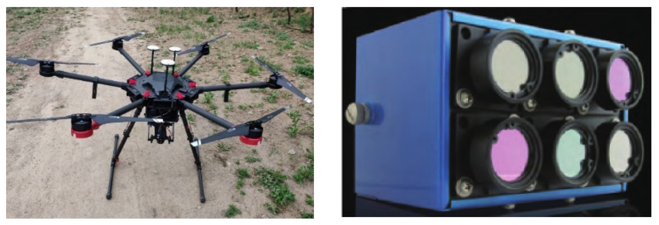
2.3.1. UAV Multispectral Image Acquisition and Preprocessing

A six-rotor M600 UAV (Dajiang Innovation Technology Co., Ltd., Shenzhen, China) was used to carry a six-channel multispectral Micro-MCA camera (Tetracam Inc., Chatsworth, CA, USA) to collect images in this study (Figure 1). This multispectral camera included six channels: B (490 nm), G (550 nm), R (680 nm), RE (720 nm), NIR800 (800 nm) and NIR900 (900 nm). Each channel was equipped with a 1.3-megapixel complementary metal oxide semiconductor (CMOS) sensor, and the resolution of each image was 1280 pixels × 1024 pixels. All UAV campaigns were undertaken in windless and clear-sky conditions (between 11:30 and 13:30) at four critical growth stages. The flight altitude was 30 m, and images were collected at a spatial resolution of 1.6 cm. A white calibration plate (100% reflection reference target) was placed in the experimental field during each flight for image radiation correction. Following data acquisition, the six bands of scattered original remote sensing images (.RAW) were synthesized in Pixel Wrench 2 software (Tetracam Inc., Chatsworth, CA, USA) to obtain multipage images (.TIF). The multipage images (.TIF) were later mosaicked, registered and orthorectified in Agisoft Photoscan software (v1.4.0, Agisoft LLC, Saint Petersburg, Russia), and a single-page image (.TIF) was obtained through splicing.

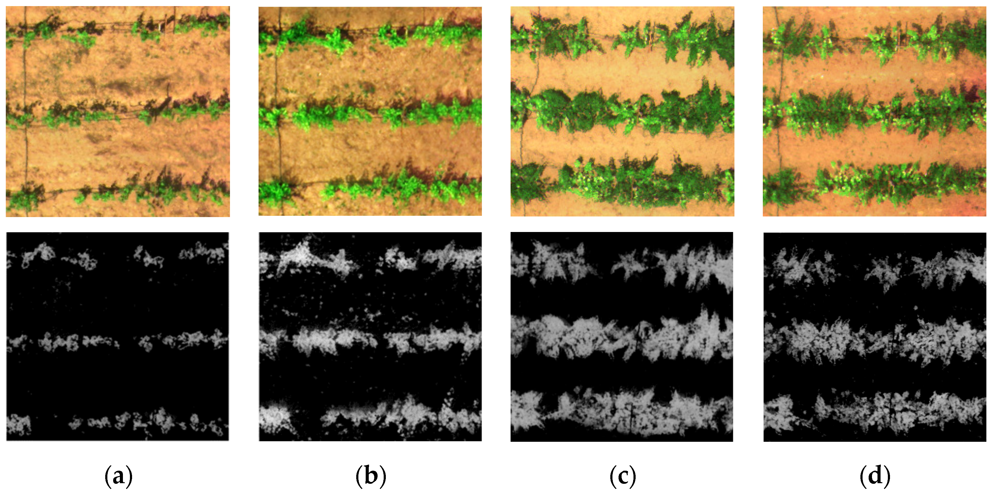
2.3.2. Extracting Band Reflectance

The single-page images (.TIF) were radiometrically corrected in MATLAB 2016a. Then, the normalized difference vegetation index (NDVI) was utilized to distinguish grape plants from other ground objects and eliminate the soil background (Figure 2). The average reflectance of the grape canopy in each plot was extracted as the spectral reflectance of the grape canopy in that plot.

2.3.3. Vegetation Indices (VIs)

In this study, based on the band range of the UAV-derived multispectral images, we selected the VIs that have been proven to be highly correlated with plant nutrient contents in the literature; in total, 11 VIs were selected, as shown in Table 3.

2.3.4. Determination of Leaf Nutrient Contents

The nutrients measured in this study included the LNC, LKC and LPC. The grape leaves samples were collected simultaneously with the UAV remote sensing. Seven to ten mature leaves were randomly picked from 3 trees in each plot and brought back to the laboratory. The leaves were washed with distilled water, placed into an oven at 105 °C for 30 min to deactivate the enzymes, and then dried to a constant weight at approximately 80 °C. The LNC and LPC were determined by the Kjeldahl method and Mo-Sb colorimetric method, respectively, with an AutoAnalyzer-III (SEAL, Norderstedt, Germany) instrument. The LKC was determined by the flame photometric method with Z-2000 flame atomic spectrophotometer (Hitachi, Tokyo, Japan).

2.4. Model Building and Data Analysis

The LNC, LPC and LKC measurements obtained in each growth stage were selected as dependent variables. The grape canopy reflectance and VIs were selected as independent variables. The number of samples obtained in the new shoot growth stage, flowering stage, fruit expansion stage and veraison and maturity stage were 252, 126, 126 and 210, respectively. Two-thirds of the obtained data in each growth stage were used as the modeling set, while 1/3 of the data were used as the verification set. The PLS, RF, SVM and ELM algorithms were applied in MATLAB R2016a to predict the LNC, LPC and LKC in the different growth stages.

2.4.1. PLS Model

The PLS method is mainly selected for modeling linear regression between multi-predictive variables and multi-response variables. PLS is a bilinear regression model, which integrates the characteristics of principal component analysis, canonical correlation analysis and linear regression analysis. The advantage of PLS is that it can handle data sets with high correlations among predictive variables.

2.4.2. RF Model

The RF is a nonlinear, multivariable statistical method. Multiple random samples are obtained through multiple bootstrap sampling, and then corresponding decision-making trees are established based on these samples, thus forming an RF algorithm for classification and regression analysis. For regression problems, the predicted value of the dependent variable is obtained from the average of the results of these decision-making trees [37]. During the regression simulation of the RF algorithm, two parameters need to be optimized: mtry (number of random variables per decision tree node) and ntree (number of decision trees generated). In this study, for each iteration, the ntree value increased from 5 to 500 at intervals of 5 for a total of 100 iterations, and the mtry value increased from 1 to m (m is the number of variables) at intervals of 1 each time for a total of m iterations. The other parameters were set to the default values.

2.4.3. SVM Model

The principle of the SVM model is to find an optimal classification surface to minimize the errors among all training samples and the classification surface. In this method, the error is calculated by the loss function. The SVM model maps data from a low-dimensional space to a high-dimensional space through a kernel function and then utilizes a representative set of support vectors to construct the prediction model. In this study, the radial basis function (RBF) was selected as the SVM kernel function, and the grid-search method of fivefold cross-validation was used to optimize the penalty factor radial basis function parameter g to [2−10, 210]. The step length was 20.5, and the optimal values of c and g values were determined by obtaining the minimum RMSE of the validation set [38].

2.4.4. ELM Model

The ELM is a new algorithm based on a single-hidden-layer feedback neural network. This model solves the problem of traditional neural networks becoming easily stuck in a local minimum error value. The ELM model can randomly generate connection weights between the input layer and hidden layers and can obtain the thresholds of the hidden layer neurons [39]. In this study, the hidden layer neurons represented the default ‘sigmoid’ activation function. The number of hidden layers was increased from 15 to 100 at intervals of 5.

2.4.5. Uncertainty Analysis

In this study, the d-factor coefficient was used to evaluate the uncertainty of the models. This evaluation was performed done by increasing and decreasing the range of 10% for each input item in MATLAB, using the Unifrnd function to generate continuous and evenly distributed random numbers, bringing the newly generated input items into the established model [40], and determining the indicative upper limit (XU) and lower limit (XL) with a 95% confidence interval. In addition, the d-factor coefficient was utilized to calculate the average width of the confidence interval, as shown in Equations (2) and (3):
d   -   factor = d X ¯ σ X ,
d X ¯ = 1 n i = 1 n   ( X Ui   -   X Li )   ,
where d X ¯ is the average distance between the indicative upper limit ( X Ui ) and the indicative lower limit ( X Li ), that is, the average width of the 95% confidence interval; n is the number of samples; and σ X is the standard deviation of the measured sap flow rate. The larger the uncertainty value is, the larger the range of the simulated values near the measured value is, the lower the accuracy of the model is, and the more unstable the model is.

2.5. Model Verification

To evaluate the accuracy of the PLS, RF, SVM and ELM model predictions, the determination coefficient (R2), relative root mean square error (RRMSE) and Willmott consistency index (WIA) were selected as evaluation indexes. The calculation formulas are presented as follows:
R 2 = i = 1 N ( P i O ¯ ) 2 i = 1 N ( O i O ¯ ) 2 ,
RRMSE = i = 1 N   ( O i   -   P i ) 2 N / P ¯ ,
WLA = 1 i = 1 N ( P i O i ) 2 i = 1 N ( | P i O i | + | O i O ¯ | ) 2
where O i and P i are the measured values and predicted values, respectively, of the leaf nutrient contents (g/kg); O ¯ and P ¯ is the mean measured value and mean predicted value, respectively, of the leaf nutrient contents (g/kg); and N is the number of samples in the prediction set.

3. Results

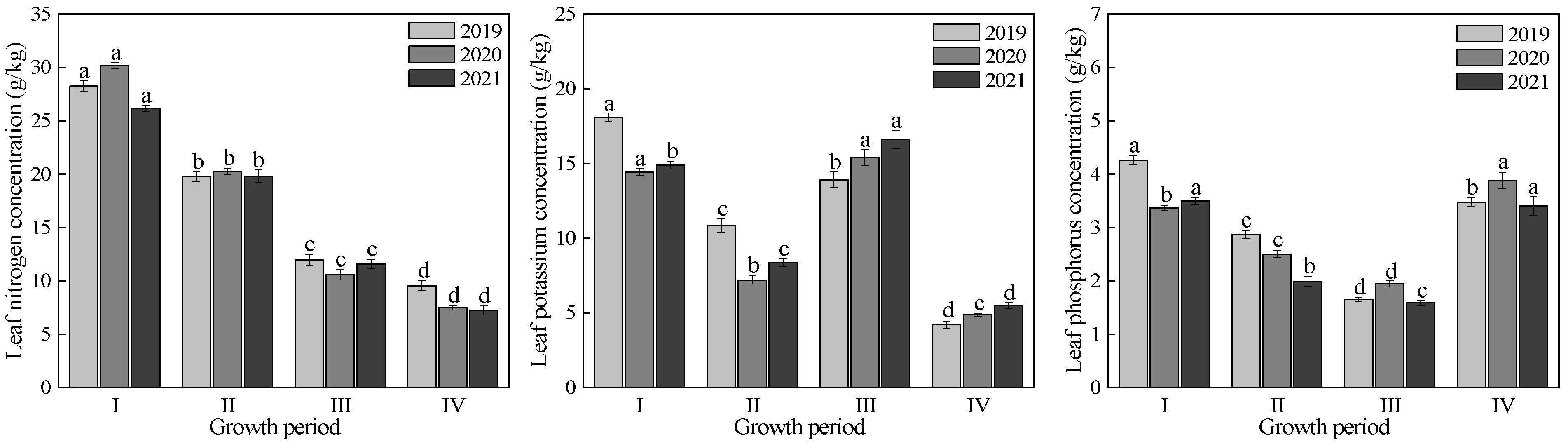
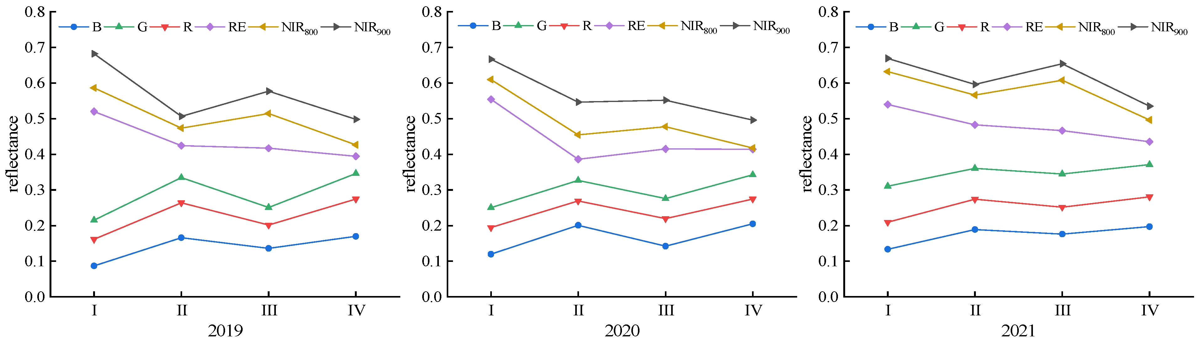
3.1. Variations in the LNC, LPC and LKC Values and Canopy Reflectance at Different Grape Growth Stages

The variations in the LNC, LKC and LPC values and the canopy reflectance at different grape growth stages from 2019 to 2021 are shown in Figure 3 and Figure 4, respectively. From 2019 to 2021, the dynamic LNC, LKC and LPC change trends observed in the grape plants throughout the whole growth period of each year were consistent. From the new shoot growth stage to fruit expansion stage, rapid decreases in the LNC were observed as soon as the grape growth period advanced. However, the LNC decreased slightly following the fruit expansion stage to veraison and maturity stage. The LKC presented a decreasing trend from the new shoot growth period to flowering period, with a sharp increase in the fruit expansion stage and a sharp decrease in the veraison and maturity stage. The LPC variation presented a decreasing trend from the new shoot growth stage to the fruit expansion stage and increased sharply in the veraison and maturity stage. These results indicated that the analyzed grape trees had high N requirements at the early growth stage, while the demands for K and P occurred mainly during the fruit expansion stage and the veraison and maturity stage, respectively. In addition, significant LNC differences were observed among each growth period (p < 0.05). There was no significant difference in the LKC between the new shoot growth period and fruit expansion period in 2020 (p > 0.05), and there was no significant difference in the LPC between the new shoot growth stage and veraison and maturity stage in 2021 (p > 0.05); however, significant differences were observed among the other growth periods (p < 0.05).
The canopy spectral reflectance variation trend observed throughout the whole grape growth period from 2019 to 2021 was nearly consistent, but obvious differences were observed between different bands in each growth stage (Figure 4). With the advancement of the grape growth period, the reflectivity of the B, G and R bands presented overall upward trends, and the reflectances of the NIR800 and NIR900 bands showed overall downward trends. However, during the fruit expansion stage, there was a slight decrease in the reflectivities of the B, G and R bands, while the reflectivities of the NIR800 and NIR900 bands increased slightly.

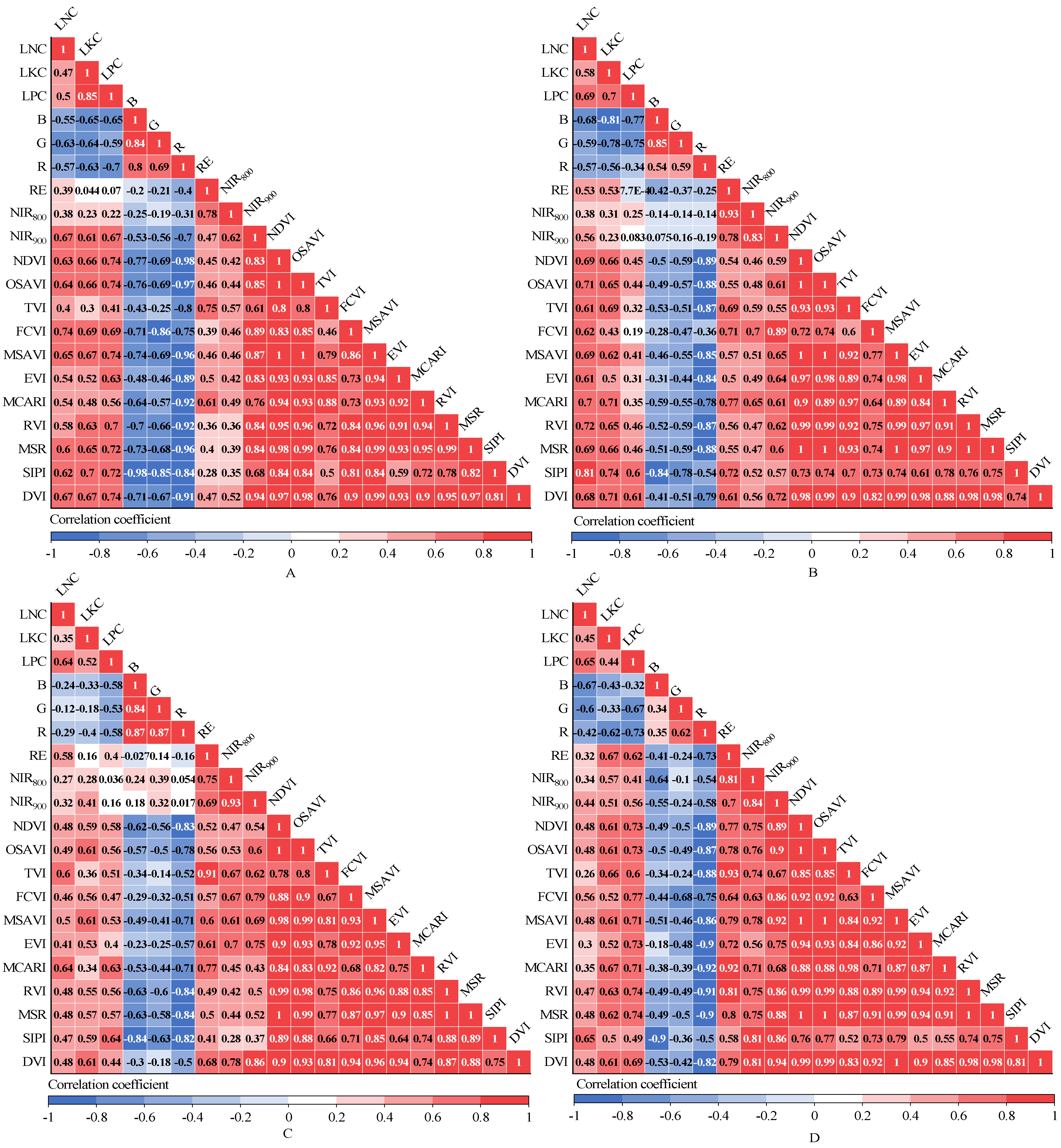
3.2. Correlation Analyses between Spectral Variables and the LNC, LKC and LPC

The correlation coefficients between spectral variables and the LNC, LKC and LPC are as shown in Figure 5. The NDVI, OSAVI, FCVI, MSAVI, MSR, SIPI and DVI had high correlations with the LNC, LKC and LPC at the new shoot growth stage; all correlation coefficients were greater than 0.60. During the flowering stage, the SIPI had the highest correlation with the LNC, while B had the highest correlation coefficients with the LKC and LPC. At the fruit expansion stage, the correlation coefficients of the MCARI and TVI with the LNC, the correlation coefficients of the MSAVI, DVI and OSAVI with the LKC, and the correlation coefficients of the SIPI and MCARI with the LPC were all above 0.60. At the veraison and maturity stage, the B, RE and FCVI had the highest correlation coefficients with the LNC, LKC and LPC, respectively. In addition, the correlation coefficients between the spectral variables and the LNC, LKC and LPC derived during the fruit expansion period were lower than those obtained in the other three growth periods.

3.3. LNC, LKC, and LPC Prediction Models Constructed Based on Different Spectral Variables

On the basis of the analysis performed in Section 3.2, according to the correlation coefficients of the analyzed spectral variables with the LNC, LKC and LPC, the 17 spectral variables were sorted to reduce the number of spectral variables input to the RF, PLS, SVR and ELM models. Then, LNC, LKC and LPC estimation models were established. The model accuracy evaluation indices and the number of input variables were comprehensively analyzed, as shown in Table 4, Table 5 and Table 6. The results showed that the numbers of spectral variables used in the optimal LNC, LKC and LPC prediction models constructed using different algorithms at different growth stages were also different. For the RF model, the numbers of spectral variables input to the optimal LNC prediction model at the new shoot growth stage, flowering stage, fruit expansion stage and veraison and maturity stage were 4, 1, 4 and 3, respectively; the numbers of spectral variables input to the optimal LKC prediction model at these stages were 4, 3, 4 and 6, respectively; and the numbers of spectral variables input to the optimal LPC prediction model were 6, 4, 4 and 2, respectively. Similarly, for the PLS model, 1, 2, 4 and 3 spectral variables (for the LNC prediction model), 3, 3, 3 and 3 spectral variables (for the LKC prediction model), and 3, 3, 3 and 3 spectral variables (for the LPC prediction model) were selected due to their optimal modeling effects; for the SVR model, 6, 5, 5 and 3 spectral variables (for the LNC prediction model), 5, 1, 4 and 3 spectral variables (for the LKC prediction model), and 3, 4, 7 and 3 spectral variables (for the LPC prediction model) were selected for modeling. For the ELM model, 7, 6, 3 and 6 spectral variables (for the LNC prediction model), 5, 4, 7 and 7 spectral variables (for the LKC prediction model), and 7, 4, 4 and 6 spectral variables (for the LPC prediction model) were selected to obtain the optimal modeling effect.
The results obtained using the models constructed based on the optimal numbers of predictive variables derived in the four growth stages are shown in Table 7. Compared to the RF, PLS and SVM models, the simulation results of the ELM model were more accurate when predicting the LNC, and the R2 values of the ELM model at the new shoot growth, flowering, fruit expansion and veraison and maturity periods were 2.256–25.174% higher, 23.404–74.249% higher, 11.019–31.057% higher and 14.960–62.786% higher, respectively, than those of these other models; In addition, the RRMSE values were 3.226–31.818% lower, 25.263–38.793% lower, 7.821–27.313% lower and 37.222–53.688% lower, respectively, than those of the other models, and the WIA values were all greater than 0.85. When predicting the LKC, compared to the other three models, the RF model had the best modeling effect during the new shoot growth period, the ELM model had the best modeling effect during flowering and fruit expansion periods, and the SVM model had the best prediction effect during the veraison and maturity period. For predicting the LPC, compared to the RF, PLS and SVM models, the ELM model had a better prediction effect at different growth stages; the R2 values at the new shoot growth, flowering, fruit expansion and veraison and maturity stages were 3.427–11.409%, 3.000–44.561%, 13.475–29.241% and 27.888–44.320% higher, respectively, than those of the other models, while the RRMSE values were 6.400–17.606%, 3.636–34.568%, 31.429–36.170% and 1.775–16.583% lower, respectively. From the above analysis, it can be seen that the simulation results obtained for different growth stages were also different. The LNC model established based on the ELM algorithm exhibited the best prediction effect the veraison and maturity stage, followed by the flowering period, fruit expansion period and new shoot growth period. When predicting the LPC, the flowering-period model had the best prediction effect, while the new-shoot-growth-period model was the worst. In addition, Table 7 shows that among the different prediction models obtained, the LNC model constructed with the B, SIPI, G, FCVI, OSAVI and NDVI as prediction variables by the ELM algorithm had the best prediction effect during the veraison and maturity stage, exhibiting optimal correlations between the real and predicted values. The R2 value was greater than 0.85 and the RRMSE value was 0.95; thus, the model was considered reliable.

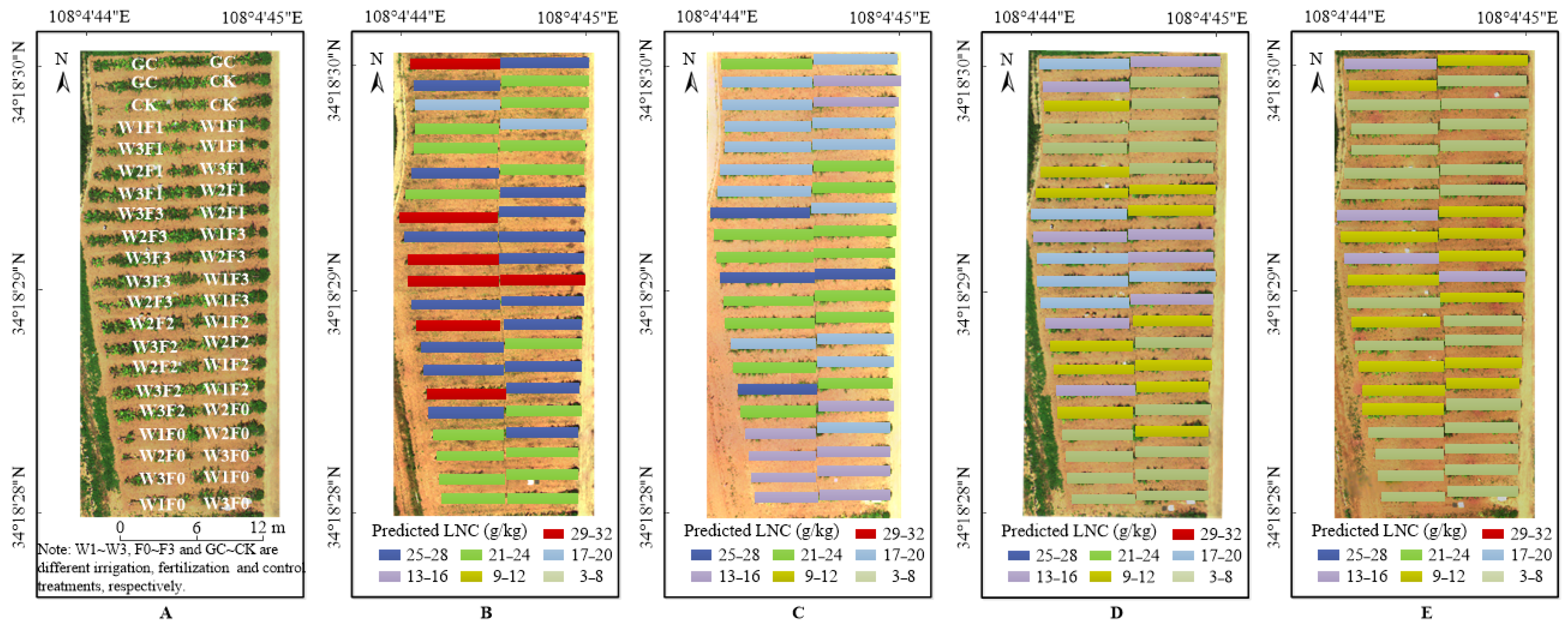
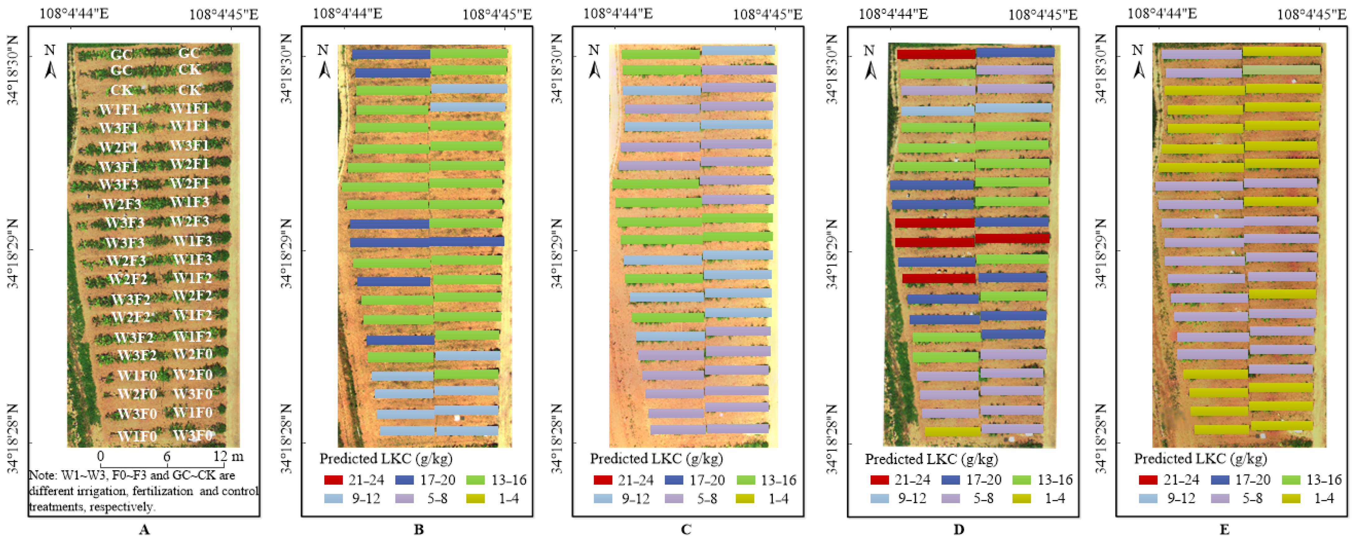
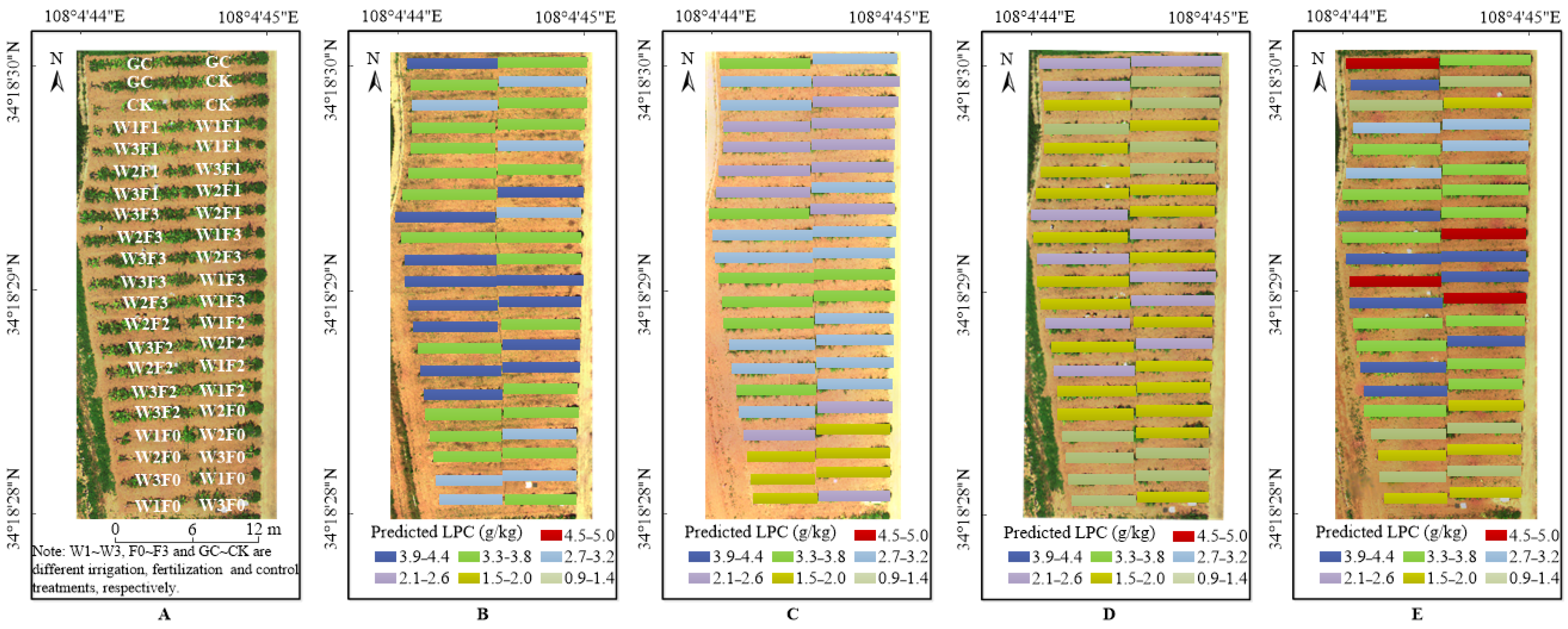
3.4. Distributions of LNC, LKC and LPC in Different Growth Stages

The optimal prediction models of LNC, LKC and LPC in each growth period were selected by R2, RRMSE and WIA shown in Table 7, and the spatial distribution of predicted results of LNC, LKC and LPC were shown in Figure 6, Figure 7 and Figure 8, respectively. It can be seen that there were differences in grape growth under different fertilization treatments. With the increase of fertilization, the nutrient content of grape leaves also showed a rising trend. The plot under different fertilization treatments could be clearly distinguished in the figure. LNC, LKC and LPC of grape were lower under F0 and CK treatments, while F3 and F2 treatments had higher nutrient content in grape leaves. It is feasible to estimate grape LNC, LKC and LPC at field scale by UAV multispectral remote sensing.

3.5. Model Uncertainty Analysis

Uncertainty analysis is performed primarily to test whether the simulation effect of a model remains stable after changing an input term and whether the model can still achieve an accurate prediction effect with the new input term. In this study, the model stability was evaluated on the basis of uncertainty analysis and the d-factor value. The d-factor values of the constructed models were obtained based on the numbers of the best predictors in the different grape growth stages, as shown in Table 8. The results suggest that the average d-factor values of the ELM and RF models were relatively small, and these models remained stable. In contrast, the d-factor value of the PLS model was large; to improve the accuracy of this model, we would need to reanalyze the data and adjust the model parameters. The uncertainty of the model also varied among different growth stages, and the uncertainty of the LNC model gradually decreased as the growth period advanced. The uncertainty of the LKC model increased among stages in the following order: flowering stage < veraison and maturity stage < fruit expansion stage < new shoot growth stage. The largest uncertainty of the LPC model was found in the new shoot growth stage, followed by the veraison and maturity stage, the flowering stage and the fruit expansion stage. The uncertainties of the LNC prediction model during the new shoot growth period and flowering period were higher than those of the LKC model and LPC model; the largest uncertainties of the LKC model and LPC model were observed in the fruit expansion stage and veraison and maturity stage, respectively.

4. Discussion

4.1. Comparison of Sensitive Spectral Variables at Different Growth Stages

In this study, we analyzed the correlations between 17 spectral variables and the nitrogen, phosphorus and potassium contents in grape leaves at different growth stages. We found that the correlation coefficients between the VIs and the nitrogen, phosphorus and potassium contents in grape leaves was the lowest at the fruit expansion stage throughout the whole grape growth period; this might have been related to the size of the grape canopy. During the new shoot growth stage, new branches grow, new leaves proliferate, and the leaf area gradually increases. After the fruit expansion stage, the leaf area of the plants is maximized and tends to stabilize. In the subsequent veraison and maturity stage, the leaves gradually turn yellow and fall off, and the effective leaf area begins to decrease. However, VIs are usually saturated in high-density vegetation canopies [41]; thus, the VIs extracted during the grape fruit expansion period were saturated in this work, resulting in the correlations between the VIs and the LNC, LKC and LPC being lower in this period than in other periods.
In addition, we found that the top 5 spectral variables related to leaf nutrient contents during the new shoot growth stage were almost for VIs (such as, DVI, MSAVI, OSAVI, FCVI, etc.) based on soil line; these soil line-based VIs were developed to minimize the influence of the soil background on the results [42]. With the advancement of the growth period, most spectral variables changed into the VIs (such as MCARI, SIPI, MSAVI, TVI, etc.) sensitive to plant nitrogen, and a small portion of these variables are VIs related to the regulation of the soil background. This shows that VIs based on the soil line can compensate for the errors caused by the soil background when the vegetation coverage is low during the new shoot growth period [43]; thus, these are the best spectral variables for predicting the leaf nutrient contents by remote sensing in the early stage of grape growth. The VIs that are sensitive to plant pigments are the key indices used to predict the nutrient contents in grape leaves from the flowering to coloring maturity stages. However, because grapes are sparsely planted fruit trees, it is necessary to partially optimize the soil background-related VIs to reduce the impact of the soil background.

4.2. Performances of Different Machine Learning Models

In this study, based on spectral indices and machine learning algorithms, we established models to estimate the LNC, LKC and LPC at different grape growth stages. We found that the prediction effects of the different analyzed machine learning algorithms were not the same, and the numbers of optimal spectral variables selected for the models were also different (as shown in Table 7). Previous studies have shown that it is difficult to estimate multitemporal changes in crop leaf nutrients with traditional VIs because these VIs appear saturated and have low sensitivities during the reproductive crop stage [44,45]. However, in this study, we found that it was feasible to predict the LNC, LKC and LPC at different growth stages by using multiple VIs combined with machine learning models. This may have been because the analyzed VIs were calculated using different band reflectances, and the sensitivity differences among the LNC, LKC and LPC may be obvious at different growth stages. Moreover, compared to PLS, a linear machine learning algorithm, the nonlinear RF, SVM and ELM machine learning algorithms had better prediction accuracies, while the ELM model had the best overall prediction effect, which may have been related to the number of spectral variables used in the modeling process. The analysis results listed in Table 7 show that the number of spectral variables used to establish the ELM model was generally greater than those of the other three models, indicating that under the same conditions, the ELM model can use more spectral information than the other three models, making this model the most accurate. In addition, the prediction effect of the ELM model at the fruit expansion stage was better than that of this model at the new shoot growth stage. Therefore, combining VIs with machine learning algorithms such as ELM is helpful for overcoming the saturation problem associated with using single VIs to obtain estimations during the grape fruit expansion stage.
By comparing the models constructed to predict the LNC, LKC and LPC at different grape growth stages, we found that the prediction accuracies at the new shoot growth period were generally low; this may have been because grapes are perennial crops, and branches are artificially pruned after each harvest period, so large growth differences occur during the early growth period associated with highly variable nutrient absorption among trees. In this study, the determination of the LNC, LPC and LKC values was based on the leaf scale, while the spectral indices were calculated based on the canopy scale, thus affecting the accuracy of the models. Similarly, the prediction accuracy of the LKC model at the fruit expansion stage and that of the LPC model at the veraison and maturity stages were low, which may have been because grape trees absorb a large amount of K at the fruit expansion stage and absorb a large amount of P at the veraison and maturity stage (Figure 3). This may have caused the potassium and phosphorus contents of grape leaves to fluctuate greatly and increased the errors caused by mismatches between the leaf and canopy scales, resulting in the low model accuracies. In a follow-up study, the leaf area or its related indicators should be considered in the model construction process to improve the resulting prediction accuracy.

4.3. Research Limitations and Future Prospects

UAV multispectral technology represents a new remote sensing method that is critical in large-scale precision agriculture research. This study was carried out under field experimental conditions. Statistically, obtaining more samples based on larger regions would improve the generalization ability of the constructed models. In this study, we found that VIs with high correlations with the LNC, LKC and LPC differed among different growth stages, indicating that it is challenging to select suitable VIs for estimating physiological growth parameters of the same crop at different growth stages [46]. In addition, the amount of nitrogen, potassium and phosphorus fertilizer applied to the field increased and decreased simultaneously in this research. It is difficult to distinguish the reflectance effect and find the sensitive spectral characteristics of a certain element, considering the influence of other nutrients on the spectrum. Therefore, it is necessary to set nitrogen, phosphorus or potassium fertilizer gradient while keeping others consistent to further explore the sensitive spectral characteristics of N, K and P in future research.
In this study, multiple VIs were combined with RF, SVM and ELM models to better predict the LNC, LPC and LKC values of grapes at different growth stages; we determined the optimal VIs for predicting the nutrient contents of grape leaves at different growth stages. The nutrient content of grape leaves at different stages obtained by UAV multispectral remote sensing was used to determine the nutrient deficiency status of grape plants at different growth stages. This provides support for field fertilization decision-making in vineyards at key growth stages. In future work, spectral variable combinations should be further studied, and the scale problem should be fully considered to obtain an improved universal estimation model.

5. Conclusions

In this study, based on UAV-derived multispectral images, we performed correlation analyses between spectral variables and leaf nitrogen, phosphorus and potassium contents at different grape growth stages, and the optimal spectral variable combinations for estimating the various leaf nutrient contents were selected. The PLS, RF, SVM and ELM models were used for modeling, and the model uncertainties were evaluated. The grape LNC, LPC and LKC values were effectively estimated using these models. The results showed that combining spectral variables with the ELM model resulted in a model that could best predict the LNC, LKC and LPC values at different growth stages. The best prediction result was obtained using the LPC model with the B, SIPI, G, FCVI, OSAVI and NDVI input as prediction variables at the veraison and maturity stages. The R2, RRMSE and WIA values obtained for this model were 0.853, 0.113 and 0.955, respectively. The d-factor value of the model was 0.157; the model was stable and reliable. This study proved the feasibility of using combinations of spectral indices and machine learning algorithms to establish grape LNC, LPC and LKC prediction models, thus providing data support for scientific fertilization and the decision-making management of field-grown grapes.

Author Contributions

Conceptualization, X.P. and X.H.; methodology, X.P.; software, X.P.; validation, X.P., D.C. and Z.Z. (Zhenjiang Zhou); formal analysis, Z.Z. (Zhitao Zhang) and C.X.; data curation, C.X., Q.Z. and F.W.; writing original draft preparation, X.P.; writing review and editing, X.P., X.H., D.C. and Z.Z. (Zhitao Zhang); funding acquisition, X.H. All authors have read and agreed to the published version of the manuscript.

Funding

This research was funded by the National Key Research and Development Program Project of China, grant number 2017YFD0201508, and the Science and Technology Department of Guangdong Province, grant number 2019B020216001.

Data Availability Statement

No new data were created or analyzed in this study. Data sharing is not applicable to this article.

Acknowledgments

We would like to thank the Key Laboratory of Agricultural soil and water engineering in Arid and Semiarid Areas for providing the equipment and materials used for experiments.

Conflicts of Interest

The authors declare no conflict of interest.

References

  1. FAO. Food and Agriculture Organization of the United Nations. 2019. Available online: http://www.fao.org/faostat/en/#data (accessed on 22 March 2022).
  2. Jinglin, L.; Hongju, Z.; Zhifang, L. Effects of Application of Potassium on the Yield and Quality of Grape in Greenhouse. Chin. J. Soil Sci. 2015, 46, 694–697. [Google Scholar]
  3. Lianjun, W.; Chenghan, W.; Jianlei, Q.; Yingkui, X. Effects of Water and Fertilizer Quality of Grape under Drip Coupling on Growth, Yield and Irrigation with Film Mulching. Trans. Chin. Soc. Agric. Mach. 2016, 47, 113–119. [Google Scholar] [CrossRef]
  4. Berger, K.; Verrelst, J.; Féret, J.-B.; Wang, Z.; Wocher, M.; Strathmann, M.; Danner, M.; Mauser, W.; Hank, T. Crop nitrogen monitoring: Recent progress and principal developments in the context of imaging spectroscopy missions. Remote Sens. Environ. 2020, 242, 111758. [Google Scholar] [CrossRef]
  5. Haboudane, D.; Miller, J.R.; Tremblay, N.; Zarco-Tejada, P.J.; Dextraze, L. Integrated narrow-band vegetation indices for prediction of crop chlorophyll content for application to precision agriculture. Remote Sens. Environ. 2002, 81, 416–426. [Google Scholar] [CrossRef]
  6. Pengfei, W.; Xingang, X.; Zhongyuan, L.; Guijun, Y.; Zhenhai, L.; Haikuan, F.; Guo, C.; Lingling, F.; Yulong, W.; Shuaibing, L. Remote sensing estimation of nitrogen content in summer maize leaves based on multispectral images of UAV. Trans. Chin. Soc. Agric. Eng. 2019, 35, 126–133, 335. [Google Scholar]
  7. Deng, L.; Mao, Z.; Li, X.; Hu, Z.; Duan, F.; Yan, Y. UAV-based multispectral remote sensing for precision agriculture: A comparison between different cameras. ISPRS J. Photogramm. Remote Sens. 2018, 146, 124–136. [Google Scholar] [CrossRef]
  8. Barbedo, J. A Review on the Use of Unmanned Aerial Vehicles and Imaging Sensors for Monitoring and Assessing Plant Stresses. Drones 2019, 3, 40. [Google Scholar] [CrossRef] [Green Version]
  9. Wang, H.; Mortensen, A.K.; Mao, P.; Boelt, B.; Gislum, R. Estimating the nitrogen nutrition index in grass seed crops using a UAV-mounted multispectral camera. Int. J. Remote Sens. 2019, 40, 2467–2482. [Google Scholar] [CrossRef]
  10. Zheng, H.; Li, W.; Jiang, J.; Liu, Y.; Cheng, T.; Tian, Y.; Zhu, Y.; Cao, W.; Zhang, Y.; Yao, X. A Comparative Assessment of Different Modeling Algorithms for Estimating Leaf Nitrogen Content in Winter Wheat Using Multispectral Images from an Unmanned Aerial Vehicle. Remote Sens. 2018, 10, 2026. [Google Scholar] [CrossRef] [Green Version]
  11. Cilia, C.; Panigada, C.; Rossini, M.; Meroni, M.; Busetto, L.; Amaducci, S.; Boschetti, M.; Picchi, V.; Colombo, R. Nitrogen Status Assessment for Variable Rate Fertilization in Maize through Hyperspectral Imagery. Remote Sens. 2014, 6, 6549. [Google Scholar] [CrossRef] [Green Version]
  12. Huang, S.; Miao, Y.; Yuan, F.; Gnyp, M.L.; Yao, Y.; Cao, Q.; Wang, H.; Lenz-Wiedemann, V.I.S.; Bareth, G. Potential of RapidEye and WorldView-2 Satellite Data for Improving Rice Nitrogen Status Monitoring at Different Growth Stages. Remote Sens. 2017, 9, 227. [Google Scholar] [CrossRef] [Green Version]
  13. Chlingaryan, A.; Sukkarieh, S.; Whelan, B. Machine learning approaches for crop yield prediction and nitrogen status estimation in precision agriculture: A review. Comput. Electron. Agric. 2018, 151, 61–69. [Google Scholar] [CrossRef]
  14. Liakos, K.G.; Busato, P.; Moshou, D.; Pearson, S.; Bochtis, D. Machine Learning in Agriculture: A Review. Sensors 2018, 18, 2674. [Google Scholar] [CrossRef] [PubMed] [Green Version]
  15. Ali, I.; Greifeneder, F.; Stamenkovic, J.; Neumann, M.; Notarnicola, C. Review of Machine Learning Approaches for Biomass and Soil Moisture Retrievals from Remote Sensing Data. Remote Sens. 2015, 7, 15841. [Google Scholar] [CrossRef] [Green Version]
  16. Hansen, P.M.; Schjoerring, J.K. Reflectance measurement of canopy biomass and nitrogen status in wheat crops using normalized difference vegetation indices and partial least squares regression. Remote Sens. Environ. 2003, 86, 542–553. [Google Scholar] [CrossRef]
  17. Jin, J.; Huang, N.; Huang, Y.; Yan, Y.; Zhao, X.; Wu, M. Proximal Remote Sensing-Based Vegetation Indices for Monitoring Mango Tree Stem Sap Flux Density. Remote Sens. 2022, 14, 1483. [Google Scholar] [CrossRef]
  18. Wang, F.; Yang, M.; Ma, L.; Zhang, T.; Qin, W.; Li, W.; Zhang, Y.; Sun, Z.; Wang, Z.; Li, F.; et al. Estimation of Above-Ground Biomass of Winter Wheat Based on Consumer-Grade Multi-Spectral UAV. Remote Sens. 2022, 14, 1251. [Google Scholar] [CrossRef]
  19. Wang, J.; Zhou, Q.; Shang, J.; Liu, C.; Zhuang, T.; Ding, J.; Xian, Y.; Zhao, L.; Wang, W.; Zhou, G.; et al. UAV- and Machine Learning-Based Retrieval of Wheat SPAD Values at the Overwintering Stage for Variety Screening. Remote Sens. 2021, 13, 5166. [Google Scholar] [CrossRef]
  20. Liu, X.; Lv, Q.; He, S.; Yi, S.; Xie, R.; Zheng, Y.; Hu, D.; Wang, Z.; Deng, j. Estimation of nitrogen and pigments content in citrus canopy by low-altitude remote sensing. J. Remote Sens. 2015, 19, 1007–1018. [Google Scholar] [CrossRef]
  21. Liu, H.; Zhu, H.; Wang, P. Quantitative modelling for leaf nitrogen content of winter wheat using UAV-based hyperspectral data. Int. J. Remote Sens. 2017, 38, 2117–2134. [Google Scholar] [CrossRef]
  22. Li, M.; Zhu, X.; Bai, X.; Peng, Y.; Tian, Z.; Jiang, Y. Remote Sensing Inversion of Nitrogen Content in Apple Canopy Based on Shadow Removal in UAV Multi-Spectral Remote Sensing Images. Sci. Agric. Sin. 2021, 54, 2084–2094. [Google Scholar] [CrossRef]
  23. Shrestha, D.L.; Kayastha, N.; Solomatine, D.P. A novel approach to parameter uncertainty analysis of hydrological models using neural networks. Hydrol. Earth Syst. Sci. Discuss. 2009, 6, 1235–1248. [Google Scholar] [CrossRef] [Green Version]
  24. Chancia, R.; Bates, T.; Vanden Heuvel, J.; van Aardt, J. Assessing Grapevine Nutrient Status from Unmanned Aerial System (UAS) Hyperspectral Imagery. Remote Sens. 2021, 13, 4489. [Google Scholar] [CrossRef]
  25. Moghimi, A.; Pourreza, A.; Zuniga-Ramirez, G.; Williams, L.E.; Fidelibus, M.W. A Novel Machine Learning Approach to Estimate Grapevine Leaf Nitrogen Concentration Using Aerial Multispectral Imagery. Remote Sens. 2020, 12, 3515. [Google Scholar] [CrossRef]
  26. Peng, X.; Hu, X.; Chen, D.; Zhou, Z.; Guo, Y.; Deng, X.; Zhang, X.; Yu, T. Prediction of Grape Sap Flow in a Greenhouse Based on Random Forest and Partial Least Squares Models. Water 2021, 13, 3078. [Google Scholar] [CrossRef]
  27. Tucker, C.J. Red and photographic infrared linear combinations for monitoring vegetation. Remote Sens. Environ. 1979, 8, 127–150. [Google Scholar] [CrossRef] [Green Version]
  28. Rondeaux, G.; Steven, M.; Baret, F. Optimization of soil-adjusted vegetation indices. Remote Sens. Environ. 1996, 55, 95–107. [Google Scholar] [CrossRef]
  29. Broge, N.H.; Leblanc, E. Comparing prediction power and stability of broadband and hyperspectral vegetation indices for estimation of green leaf area index and canopy chlorophyll density. Remote Sens. Environ. 2001, 76, 156–172. [Google Scholar] [CrossRef]
  30. Jiang, J.; Cai, W.; Zheng, H.; Cheng, T.; Tian, Y.; Zhu, Y.; Ehsani, R.; Hu, Y.; Niu, Q.; Gui, L.; et al. Using Digital Cameras on an Unmanned Aerial Vehicle to Derive Optimum Color Vegetation Indices for Leaf Nitrogen Concentration Monitoring in Winter Wheat. Remote Sens. 2019, 11, 2667. [Google Scholar] [CrossRef] [Green Version]
  31. Qi, J.G.; Chehbouni, A.R.; Huete, A.R.; Kerr, Y.H.; Sorooshian, S. A Modified Soil Adjusted Vegetation Index. Remote Sens. Environ. 1994, 48, 119–126. [Google Scholar] [CrossRef]
  32. Huete, A.; Didan, K.; Miura, T.; Rodriguez, E.P.; Gao, X.; Ferreira, L.G. Overview of the radiometric and biophysical performance of the MODIS vegetation indices. Remote Sens. Environ. 2002, 83, 195–213. [Google Scholar] [CrossRef]
  33. Daughtry, C.S.T.; Walthall, C.L.; Kim, M.S.; de Colstoun, E.B.; McMurtrey, J.E. Estimating Corn Leaf Chlorophyll Concentration from Leaf and Canopy Reflectance. Remote Sens. Environ. 2000, 74, 229–239. [Google Scholar] [CrossRef]
  34. Jordan, C.F. Derivation of Leaf-Area Index from Quality of Light on the Forest Floor. Ecology 1969, 50, 663–666. [Google Scholar] [CrossRef]
  35. Chen, J.M. Evaluation of Vegetation Indices and a Modified Simple Ratio for Boreal Applications. Can. J. Remote Sens. 1996, 22, 229–242. [Google Scholar] [CrossRef]
  36. Peñuelas, J.; Gamon, J.A.; Fredeen, A.L.; Merino, J.; Field, C.B. Reflectance indices associated with physiological changes in nitrogen- and water-limited sunflower leaves. Remote Sens. Environ. 1994, 48, 135–146. [Google Scholar] [CrossRef]
  37. Breiman, L. Random forests. Mach. Learing 2001, 45, 5–32. [Google Scholar] [CrossRef] [Green Version]
  38. Bingmei, C.; Xiaoping, F.; Zhiming, Z.; Xuerong, L. The principle and prospect of support vector machine. Manuf. Autom. 2010, 32, 136–138. [Google Scholar] [CrossRef]
  39. Guo, L.; Fu, P.; Shi, T.; Chen, Y.; Zhang, H.; Meng, R.; Wang, S. Mapping field-scale soil organic carbon with unmanned aircraft system-acquired time series multispectral images. Soil Tillage Res. 2020, 196, 104477. [Google Scholar] [CrossRef]
  40. Du, B.; Hu, X.; Wang, W.; Ma, L.; Zhou, S. Stem flow influencing factors sensitivity analysis and stem flow model applicability in filling stage of alternate furrow irrigated maize. Sci. Agric. Sin. 2018, 51, 233–245. [Google Scholar]
  41. Sun, G.; Jiao, Z.; Zhang, A.; Li, F.; Fu, H.; Li, Z. Hyperspectral image-based vegetation index (HSVI): A new vegetation index for urban ecological research. Int. J. Appl. Earth Obs. Geoinf. 2021, 103, 102529. [Google Scholar] [CrossRef]
  42. Barillé, L.; Mouget, J.-L.; Méléder, V.; Rosa, P.; Jesus, B. Spectral response of benthic diatoms with different sediment backgrounds. Remote Sens. Environ. 2011, 115, 1034–1042. [Google Scholar] [CrossRef]
  43. Fenling, L.; Qingrui, C.; Jian, S.; Li, W. Remote sensing estimation of winter wheat leaf nitrogen content based on GF-1 satellite data. Trans. Chin. Soc. Agric. Eng. 2016, 32, 157–164. [Google Scholar] [CrossRef]
  44. Luo, S.; He, Y.; Li, Q.; Jiao, W.; Zhu, Y.; Zhao, X. Nondestructive estimation of potato yield using relative variables derived from multi-period LAI and hyperspectral data based on weighted growth stage. Plant Methods 2020, 16, 150. [Google Scholar] [CrossRef] [PubMed]
  45. Nguy-Robertson, A.; Gitelson, A.; Peng, Y.; Viña, A.; Arkebauer, T.; Rundquist, D. Green Leaf Area Index Estimation in Maize and Soybean: Combining Vegetation Indices to Achieve Maximal Sensitivity. Agron. J. 2012, 104, 1336–1347. [Google Scholar] [CrossRef] [Green Version]
  46. Hatfield, J.L.; Prueger, J.H. Value of Using Different Vegetative Indices to Quantify Agricultural Crop Characteristics at Different Growth Stages under Varying Management Practices. Remote Sens. 2010, 2, 562. [Google Scholar] [CrossRef] [Green Version]
Figure 1. M600 UAV and Micro-MCA multispectral camera.
Remotesensing 14 02659 g001
Figure 2. (a) Effects of eliminating soil background at new shoot growth stage (8 May 2021); (b) effects of eliminating soil background at flowering stage (31 May 2021); (c) effects of eliminating soil background at fruit expansion stage (22 June 2021); (d) effects of eliminating soil background at veraison and maturity stage (23 July 2021).
Remotesensing 14 02659 g002
Figure 3. Variations in the LNC, LKC and LPC values (different small letters indicate significant difference at 0.05 level) at different grape growth stages (Ⅰ, Ⅱ, Ⅲ and Ⅳ represent the new shoot growth stage, flowering stage, fruit expansion stage and veraison and maturity stage, respectively).
Remotesensing 14 02659 g003
Figure 4. Variations in the canopy reflectance at different grape growth stages (Ⅰ, Ⅱ, Ⅲ and Ⅳ represent the new shoot growth stage, flowering stage, fruit expansion stage and veraison and maturity stage, respectively).
Remotesensing 14 02659 g004
Figure 5. (A) Correlation coefficients between spectral variables and the LNC, LKC, LPC in the new shoot growth stage. (B) Correlation coefficients between spectral variables and the LNC, LKC, LPC in the flowering stage. (C) Correlation coefficients between spectral variables and the LNC, LKC, LPC in the fruit expansion stage. (D) Correlation coefficients between spectral variables and the LNC, LKC, LPC in the veraison and maturity stage.
Remotesensing 14 02659 g005
Figure 6. (A) Distribution map of grape with different treatments based on UAV image (22 June 2021). (B) LNC distribution map of grape in the new shoot growth stage based on UAV image (8 May 2021). (C) LNC distribution map of grape in the flowering stage based on UAV image (31 May 2021). (D) LNC distribution map of grape in the fruit expansion stage based on UAV image (22 June 2021). (E) LNC distribution map of grape in the veraison and maturity stage based on UAV image (23 July 2021).
Remotesensing 14 02659 g006
Figure 7. (A) Distribution map of grape with different treatments based on UAV image (22 June 2021). (B) LKC distribution map of grape in the new shoot growth stage based on UAV image (8 May 2021). (C) LKC distribution map of grape in the flowering stage based on UAV image (31 May 2021). (D) LKC distribution map of grape in the fruit expansion stage based on UAV image (22 June 2021). (E) LKC distribution map of grape in the veraison and maturity stage based on UAV image (23 July 2021).
Remotesensing 14 02659 g007
Figure 8. (A) Distribution map of grape with different treatments based on UAV image (22 June 2021). (B) LPC distribution map of grape in the new shoot growth stage based on UAV image (8 May 2021). (C) LPC distribution map of grape in the flowering stage based on UAV image (31 May 2021). (D) LPC distribution map of grape in the fruit expansion stage based on UAV image (22 June 2021). (E) LPC distribution map of grape in the veraison and maturity stage based on UAV image (23 July 2021).
Remotesensing 14 02659 g008
Table 1. Date of grape growth stage partition and image acquisition during 2019–2021.
Growth StageDate of Grape Growth Stage PartitionDate of Image Acquisition
201920202021201920202021
New shoot growth stage4/13–5/144/10–5/184/15–5/214/24; 5/95/5; 5/145/8; 5/20
Flowering stage5/15–5/255/19–5/295/22–6/15/225/265/31
Fruit expansion stage5/26–7/115/30–7/126/2–7/107/66/7; 6/146/10; 6/22
Veraison and maturity stage7/12–8/197/13–8/217/11–8/157/237/287/23
Table 2. Irrigation and fertilization of grapevine at different growth stage in 2019–2021.
TreatmentIrrigation Quantity
(m3/hm2)
Fertilizer Amount (kg/hm2)
New Shoot Growth Stage
N + P2O5 + K2O
Fruit Expanding Stage
N+ P2O5 + K2O
Veraison and Maturity Stage
N + P2O5 + K2O
W1F097.00 + 0 + 00 + 0 + 00 + 0 + 0
W1F197.046.4 + 14.0 + 27.634.8 + 28.0 + 55.234.8 + 28.0 + 55.2
W1F297.069.6 + 20.8 + 41.652.2 + 41.6 + 83.252.2 + 41.6 + 83.2
W1F397.092.8 + 27.6 + 55.669.6 + 111.2 + 52.269.6 + 111.2 + 52.2
W2F0145.00 + 0 + 00 + 0 + 00 + 0 + 0
W2F1145.046.4 + 14.0 + 27.634.8 + 28.0 + 55.234.8 + 28.0 + 55.2
W2F2145.069.6 + 20.8 + 41.652.2 + 41.6 + 83.252.2 + 41.6 + 83.2
W2F3145.092.8 + 27.6 + 55.669.6 + 111.2 + 52.269.6 + 111.2 + 52.2
W3F0193.00 + 0 + 00 + 0 + 00 + 0 + 0
W3F1193.046.4 + 14.0 + 27.634.8 + 28.0 + 55.234.8 + 28.0 + 55.2
W3F2193.069.6 + 20.8 + 41.652.2 + 41.6 + 83.252.2 + 41.6 + 83.2
W3F3193.092.8 + 27.6 + 55.669.6 + 111.2 + 52.269.6 + 111.2 + 52.2
GC193.092.8 + 27.6 + 55.669.6 + 111.2 + 52.269.6 + 111.2 + 52.2
CK00 + 0 + 00 + 0 + 00 + 0 + 0
Table 3. The formulas for VIs were used in this study.
Vegetation IndicesFormulaReferences
Normalized difference VI (NDVI) NDVI = ρ NIR   -   ρ R ρ NIR + ρ R [27]
Optimized soil adjusted VI (OSAVI) OSAVI = ρ NIR   -   ρ R ρ NIR + ρ R + 0.16 [28]
Transformed VI (TVI) TVI = ρ G   -   ρ R ρ G + ρ R [29]
False color VI (FCVI) FCVI = 1 . 5   ×   ( 2 ρ NIR + ρ B   -   2 ρ G ) 2 R G + 2 ρ B   -   2 ρ NIR + 127 . 5 [30]
Modified soil adjusted VI (MSAVI) MSAVI = 0 . 5   ×   ( 2 ρ NIR + 1   -   ( 2 ρ NIR + 1 ) 2   -   8 ( ρ NIR   -   ρ R ) [31]
Enhanced VI (EVI) EVI = 2 . 5   ×   ρ NIR   -   ρ R ρ NIR + 6 ρ R   -   7 . 5 ρ B + 1 [32]
Modified chlorophyll absorption in reflectance index (MCARI) MCARI = ρ RE   -   ρ R   -   0 . 2 ( ρ RE -   ρ G )   ×   ρ RE ρ R [33]
Ratio VI (RVI) RVI = ρ NIR ρ R [34]
Modified simple ratio (MSR) MSR = ρ NIR ρ R   -   1 ρ NIR ρ R + 1 [35]
Structure-intensive pigment index (SIPI) SIPI = ρ NIR -   ρ B ρ NIR + ρ B [36]
Difference VI (DVI) DVI = ρ NIR   -   ρ R [34]
ρ B ,   ρ G , ρ R , ρ RE and ρ NIR represent reflectance at 480 nm, 550 nm, 680 nm, 720 nm and 900 nm, respectively.
Table 4. Results analysis of LNC prediction model constructed based on different spectral variables.
ModelThe Number of VariablesNew Shoot Growth StageFlowering StageFruit Expansion StageVeraison and Maturity Stage
R2RRMSEWIAR2RRMSEWIAR2RRMSEWIAR2RRMSEWIA
PLS170.190 0.0000.002 0.218 0.0000.000 0.485 0.0000.000 0.141 0.0000.001
70.570 0.097 0.829 0.345 0.139 0.756 0.594 0.230 0.871 0.499 0.244 0.848
60.568 0.097 0.829 0.321 0.144 0.745 0.572 0.250 0.862 0.498 0.245 0.847
50.563 0.097 0.827 0.427 0.120 0.772 0.602 0.203 0.871 0.494 0.249 0.845
40.532 0.092 0.826 0.431 0.120 0.774 0.615 0.227 0.871 0.496 0.245 0.847
30.560 0.090 0.844 0.452 0.117 0.777 0.598 0.233 0.865 0.524 0.244 0.850
20.563 0.089 0.829 0.466 0.116 0.785 0.550 0.247 0.848 0.441 0.246 0.791
10.576 0.088 0.830 0.462 0.116 0.785 0.546 0.248 0.845 0.436 0.248 0.788
RF170.626 0.088 0.892 0.516 0.126 0.862 0.654 0.216 0.896 0.704 0.189 0.916
70.616 0.085 0.894 0.490 0.113 0.803 0.682 0.211 0.905 0.713 0.186 0.915
60.655 0.068 0.914 0.451 0.117 0.787 0.688 0.209 0.907 0.707 0.188 0.911
50.665 0.067 0.910 0.485 0.113 0.799 0.684 0.210 0.906 0.701 0.190 0.912
40.671 0.068 0.916 0.508 0.111 0.809 0.710 0.198 0.908 0.694 0.194 0.910
30.630 0.074 0.898 0.418 0.121 0.771 0.691 0.204 0.901 0.725 0.172 0.917
20.625 0.074 0.896 0.477 0.115 0.801 0.494 0.263 0.823 0.631 0.200 0.879
10.410 0.098 0.820 0.525 0.111 0.838 0.514 0.257 0.831 0.633 0.200 0.884
SVM170.589 0.079 0.879 0.608 0.101 0.878 0.706 0.180 0.903 0.707 0.188 0.919
70.357 0.174 0.700 0.589 0.108 0.864 0.702 0.210 0.900 0.712 0.187 0.902
60.703 0.062 0.919 0.603 0.105 0.869 0.682 0.203 0.903 0.710 0.187 0.904
50.583 0.078 0.884 0.658 0.095 0.891 0.726 0.179 0.911 0.744 0.178 0.916
40.562 0.080 0.878 0.584 0.109 0.856 0.658 0.203 0.895 0.719 0.195 0.912
30.528 0.084 0.872 0.375 0.134 0.775 0.705 0.187 0.913 0.742 0.180 0.918
20.551 0.086 0.886 0.356 0.136 0.767 0.544 0.230 0.849 0.592 0.214 0.839
10.485 0.093 0.839 0.538 0.114 0.853 0.544 0.229 0.846 0.367 0.262 0.740
ELM170.700 0.076 0.914 0.803 0.075 0.923 0.780 0.167 0.943 0.725 0.122 0.905
70.721 0.060 0.938 0.800 0.073 0.933 0.792 0.164 0.938 0.806 0.118 0.945
60.499 0.089 0.866 0.812 0.071 0.937 0.800 0.160 0.943 0.853 0.113 0.955
50.510 0.090 0.872 0.809 0.072 0.934 0.791 0.164 0.940 0.171 0.365 0.650
40.533 0.084 0.878 0.803 0.072 0.936 0.791 0.165 0.938 0.006 0.760 0.248
30.595 0.077 0.900 0.050 7.838 0.001 0.806 0.165 0.936 0.216 0.302 0.687
20.559 0.089 0.884 0.002 0.831 0.155 0.316 0.623 0.623 0.579 0.215 0.852
10.458 0.092 0.836 0.577 0.103 0.857 0.564 0.243 0.854 0.101 4.237 0.008
Table 5. Results analysis of LKC prediction model constructed based on different spectral variables.
ModelThe Number of VariablesNew Shoot Growth StageFlowering StageFruit Expansion StageVeraison and Maturity Stage
R2RRMSEWIAR2RRMSEWIAR2RRMSEWIAR2RRMSEWIA
PLS170.162 0.0000.000 0.368 0.0000.011 0.179 0.0000.002 0.318 0.0000.000
70.489 0.133 0.823 0.734 0.153 0.923 0.496 0.186 0.891 0.625 0.169 0.877
60.477 0.135 0.817 0.720 0.160 0.917 0.502 0.188 0.890 0.620 0.170 0.877
50.482 0.135 0.820 0.728 0.157 0.917 0.509 0.187 0.891 0.661 0.156 0.879
40.482 0.135 0.820 0.737 0.155 0.919 0.516 0.198 0.889 0.660 0.156 0.879
30.499 0.132 0.826 0.743 0.153 0.921 0.553 0.180 0.836 0.671 0.153 0.887
20.487 0.132 0.826 0.727 0.157 0.916 0.501 0.204 0.864 0.612 0.164 0.866
10.453 0.139 0.807 0.697 0.167 0.909 0.494 0.206 0.859 0.622 0.163 0.865
RF170.564 0.121 0.882 0.757 0.150 0.926 0.553 0.167 0.891 0.734 0.131 0.917
70.586 0.118 0.890 0.777 0.144 0.932 0.545 0.203 0.890 0.722 0.134 0.916
60.578 0.120 0.886 0.775 0.144 0.931 0.661 0.165 0.889 0.753 0.132 0.920
50.575 0.120 0.885 0.779 0.143 0.933 0.601 0.176 0.897 0.701 0.145 0.902
40.662 0.108 0.892 0.787 0.140 0.936 0.695 0.159 0.899 0.640 0.159 0.880
30.594 0.118 0.864 0.790 0.135 0.939 0.683 0.182 0.897 0.633 0.161 0.875
20.519 0.129 0.836 0.789 0.141 0.935 0.654 0.189 0.887 0.659 0.155 0.884
10.481 0.138 0.822 0.696 0.173 0.907 0.578 0.211 0.856 0.618 0.165 0.868
SVM170.624 0.115 0.879 0.774 0.154 0.926 0.530 0.219 0.879 0.755 0.151 0.910
70.549 0.138 0.855 0.744 0.161 0.913 0.546 0.218 0.870 0.806 0.131 0.925
60.639 0.113 0.888 0.723 0.166 0.906 0.545 0.217 0.869 0.816 0.116 0.945
50.640 0.113 0.889 0.720 0.166 0.906 0.573 0.200 0.860 0.805 0.135 0.928
40.581 0.126 0.859 0.654 0.185 0.880 0.591 0.181 0.835 0.680 0.173 0.866
30.611 0.115 0.861 0.594 0.200 0.858 0.519 0.199 0.867 0.692 0.170 0.871
20.488 0.139 0.825 0.660 0.202 0.867 0.550 0.192 0.877 0.697 0.168 0.874
10.481 0.139 0.828 0.720 0.160 0.916 0.525 0.202 0.870 0.647 0.176 0.852
ELM170.584 0.111 0.869 0.806 0.135 0.946 0.701 0.176 0.915 0.782 0.154 0.943
70.549 0.117 0.857 0.803 0.136 0.944 0.759 0.162 0.932 0.801 0.147 0.942
60.548 0.115 0.856 0.801 0.137 0.944 0.713 0.174 0.914 0.449 0.405 0.746
50.613 0.102 0.879 0.800 0.136 0.943 0.546 0.279 0.838 0.562 0.244 0.862
40.582 0.117 0.871 0.810 0.135 0.940 0.598 0.212 0.867 0.310 0.983 0.465
30.504 0.125 0.826 0.578 0.243 0.856 0.522 0.237 0.850 0.276 0.618 0.583
20.369 0.204 0.747 0.501 0.215 0.825 0.102 0.420 0.611 0.108 2.415 0.000
10.485 0.135 0.823 0.345 0.264 0.777 0.376 0.363 0.732 0.084 4.147 0.015
Table 6. Results analysis of LPC prediction model constructed based on different spectral variables.
ModelThe Number of VariablesNew Shoot Growth StageFlowering StageFruit Expansion StageVeraison and Maturity Stage
R2RRMSEWIAR2RRMSEWIAR2RRMSEWIAR2RRMSEWIA
PLS170.130 0.0000.002 0.026 0.0000.000 0.205 0.0000.001 0.490 0.0000.002
70.496 0.141 0.842 0.538 0.168 0.829 0.459 0.198 0.777 0.471 0.225 0.780
60.496 0.143 0.840 0.538 0.168 0.825 0.477 0.194 0.796 0.453 0.229 0.782
50.571 0.129 0.846 0.553 0.165 0.835 0.480 0.194 0.799 0.497 0.202 0.788
40.571 0.129 0.846 0.559 0.164 0.840 0.542 0.180 0.835 0.554 0.192 0.805
30.596 0.125 0.849 0.570 0.162 0.844 0.619 0.188 0.897 0.569 0.191 0.803
20.501 0.139 0.849 0.560 0.164 0.844 0.466 0.197 0.776 0.585 0.189 0.809
10.491 0.143 0.837 0.493 0.176 0.813 0.476 0.195 0.777 0.568 0.191 0.803
RF170.595 0.122 0.879 0.673 0.157 0.899 0.612 0.156 0.893 0.560 0.186 0.822
70.540 0.132 0.889 0.653 0.179 0.908 0.640 0.166 0.894 0.538 0.191 0.817
60.642 0.118 0.880 0.649 0.181 0.905 0.677 0.151 0.891 0.513 0.195 0.805
50.563 0.130 0.852 0.701 0.133 0.902 0.683 0.150 0.895 0.509 0.196 0.801
40.558 0.131 0.850 0.711 0.134 0.901 0.705 0.175 0.906 0.525 0.193 0.807
30.550 0.132 0.844 0.578 0.161 0.849 0.683 0.152 0.889 0.562 0.187 0.815
20.527 0.135 0.831 0.558 0.165 0.843 0.666 0.155 0.887 0.606 0.169 0.823
10.497 0.140 0.819 0.527 0.170 0.822 0.433 0.219 0.802 0.407 0.214 0.765
SVM170.575 0.141 0.829 0.709 0.121 0.890 0.578 0.187 0.827 0.199 0.290 0.695
70.602 0.128 0.872 0.758 0.117 0.928 0.659 0.178 0.884 0.514 0.203 0.846
60.610 0.128 0.874 0.789 0.120 0.922 0.569 0.182 0.837 0.490 0.217 0.834
50.610 0.142 0.826 0.781 0.114 0.931 0.576 0.178 0.833 0.326 0.251 0.757
40.610 0.142 0.826 0.800 0.110 0.941 0.527 0.188 0.814 0.526 0.208 0.847
30.619 0.142 0.823 0.652 0.159 0.896 0.525 0.187 0.813 0.537 0.199 0.852
20.580 0.144 0.827 0.649 0.176 0.886 0.173 0.257 0.597 0.039 0.383 0.529
10.570 0.153 0.810 0.511 0.175 0.828 0.225 0.243 0.671 0.111 1.944 0.166
ELM170.581 0.121 0.879 0.778 0.130 0.916 0.778 0.122 0.904 0.551 0.198 0.773
70.664 0.117 0.900 0.795 0.115 0.909 0.780 0.130 0.919 0.615 0.185 0.807
60.634 0.125 0.888 0.784 0.121 0.908 0.787 0.128 0.924 0.775 0.166 0.884
50.161 0.214 0.659 0.781 0.121 0.902 0.782 0.130 0.921 0.601 0.179 0.837
40.274 0.183 0.735 0.824 0.106 0.942 0.800 0.120 0.939 0.633 0.176 0.836
30.508 0.157 0.834 0.197 0.370 0.582 0.482 0.278 0.791 0.629 0.172 0.854
20.582 0.127 0.860 0.034 0.555 0.360 0.403 0.218 0.802 0.596 0.177 0.865
10.536 0.134 0.834 0.514 0.173 0.821 0.462 0.201 0.809 0.549 0.200 0.837
Table 7. Statistical analysis of prediction models constructed based on the number of the best predictors.
Growth StageModelResponse VariablesPredictive VariablesR2RRMSEWIA
New shoot growth stagePLSLNCFCVI0.5760.0880.830
LKCSIPI, FCVI, DVI0.4990.1320.826
LPCDVI, MSAVI, OSAVI0.5960.1250.849
RFLNCFCVI, DVI, NIR900, MSAVI0.6710.0680.916
LKCSIPI, FCVI, DVI, NIR9000.6620.1080.892
LPCDVI, MSAVI, OSAVI, NDVI, MSR, SIPI0.6420.1180.880
SVMLNCFCVI, DVI, NIR900, MSAVI, OSAVI, NDVI0.7030.0620.919
LKCSIPI, FCVI, DVI, NIR900, MSAVI0.6400.1130.889
LPCDVI, MSAVI, OSAVI0.6190.1420.823
ELMLNCFCVI, DVI, NIR900, MSAVI, OSAVI, NDVI, G0.7210.0600.938
LKCSIPI, FCVI, DVI, NIR900, MSAVI0.6130.1020.879
LPCDVI, MSAVI, OSAVI, NDVI, MSR, SIPI, R0.6640.1170.900
Flowering stagePLSLNCSIPI, RVI0.4660.1160.785
LKCB, G, SIPI0.7430.1530.921
LPCB, G, DVI0.5700.1620.844
RFLNCSIPI0.5250.1110.838
LKCB, G, SIPI0.7900.1350.939
LPCB, G, DVI, SIPI0.7110.1340.901
SVMLNCSIPI, RVI, OSAVI, MCARI, MSAVI0.6580.0950.891
LKCB0.7200.1600.916
LPCB, G, DVI, SIPI0.8000.1100.941
ELMLNCSIPI, RVI, OSAVI, MCARI, MSAVI, NDVI0.8120.0710.937
LKCB, G, SIPI, DVI0.8100.1350.940
LPCB, G, DVI, SIPI0.8240.1060.942
Fruit expansion stagePLSLNCMCARI, TVI, RE, MSAVI0.6150.2270.871
LKCMSAVI, DVI, OSAVI0.5530.180.836
LPCSIPI, MCARI, R0.6190.1880.897
RFLNCMCARI, TVI, RE, MSAVI0.7100.1980.908
LKCMSAVI, DVI, OSAVI, NDVI0.6950.1590.899
LPCSIPI, MCARI, R, B0.7050.1750.906
SVMLNCMCARI, TVI, RE, MSAVI, OSAVI0.7260.1790.911
LKCMSAVI, DVI, OSAVI, NDVI0.5910.1810.835
LPCSIPI, MCARI, R, B, NDVI, MSR, OSAVI0.6590.1780.884
ELMLNCMCARI, TVI, RE0.8060.1650.936
LKCMSAVI, DVI, OSAVI, NDVI, SIPI, MSR, FCVI0.7590.1620.932
LPCSIPI, MCARI, R, B0.8000.1200.939
Veraison and maturity stagePLSLNCB, SIPI, G0.5240.2440.850
LKCRE, MCARI, TVI0.6710.1530.887
LPCFCVI, RVI, MSR0.5850.1890.809
RFLNCB, SIPI, G0.7250.1720.917
LKCRE, MCARI(6)0.7530.1320.92
LPCFCVI, RVI0.6060.1690.823
SVMLNCB, SIPI, G0.7420.1800.918
LKCRE, MCARI, TVI, RVI, MSR, R0.8160.1160.945
LPCFCVI, RVI, MSR0.5370.1990.852
ELMLNCB, SIPI, G, FCVI, OSAVI, NDVI0.8530.1130.955
LKCRE, MCARI, TVI, RVI, MSR, R, MSAVI0.8010.1470.942
LPCFCVI, RVI, MSR, NDVI, EVI, R0.7750.1660.884
Table 8. Uncertainty measurement parameter (d-factor) for different models.
ModelResponse Variablesd-Factor
New Shoot Growth StageFlowering StageFruit Expansion StageVeraison and Maturity StageAverage Value of XiAverage Value
PLSLNC0.6630.2920.2740.1860.3540.319
LKC0.5150.1680.2880.1950.292
LPC0.4820.2120.1950.3560.311
RFLNC0.6340.2910.2490.1630.3340.302
LKC0.4890.1600.2800.1940.281
LPC0.4680.1970.1870.3100.291
SVMLNC0.6460.2850.2700.1600.3400.307
LKC0.5020.1710.2880.1890.288
LPC0.4760.1880.1820.3230.292
ELMLNC0.6210.2710.2670.1570.3290.301
LKC0.5120.1640.2740.2030.288
LPC0.4870.1860.1800.2900.286
Publisher’s Note: MDPI stays neutral with regard to jurisdictional claims in published maps and institutional affiliations.

