Spatiotemporal Change Detection of Coastal Wetlands Using Multi-Band SAR Coherence and Synergetic Classification

Abstract

Synthetic aperture radar (SAR) signal can penetrate clouds and some vegetation canopies in all weather, and therefore, provides an important measurement tool for change detection and sustainable development of coastal wetland environments and ecosystems. However, there are a few quantitative estimations about the spatiotemporal coherence change with multi-band SAR images in complex coastal wetland ecosystems of the Yellow River Delta (YRD). In this study, C-band Sentinel-1 and L-band ALOS-2 PALSAR data were used to detect the spatiotemporal distribution and change pattern of interferometric coherence in the coastal wetlands of the YRD. The results show that the temporal baseline has a greater impact on the interferometric coherence than the perpendicular baseline, especially for short wavelength C-band SAR. Furthermore, the OTSU algorithm was proven to be able to distinguish the changing regions. The coherence mean and standard deviation values of different land cover types varied significantly in different seasons, while the minimum and maximum coherence changes occurred in February and August, respectively. In addition, considering three classical machine learning algorithms, namely naive Bayes (NB), random forest (RF), and multilayer perceptron (MLP), we proposed a method of synergetic classification with SAR coherence, backscatter intensity, and optical images for coastal wetland classification. The multilayer perceptron algorithm performs the best in synergetic classification with an overall accuracy of 98.3%, which is superior to a single data source or the other two algorithms. In this article, we provide an alternative cost-effective method for coastal wetland change detection, which contributes to more accurate dynamic land cover classification and to an understanding of the response mechanism of land features to climate change and human activities.

1. Introduction

Coastal wetlands are transitional zones between terrestrial and aquatic regions that are permanently or temporarily covered with shallow water [1], and which are extremely important natural ecosystems on the earth. Their functions include protecting biodiversity, filtering sediments and toxins [2], improving climate, regulating runoff, and providing an ecological buffer to protect shoreline from storm surge and costal erosion [3,4]. In recent years, global wetlands have been affected by both human overdevelopment and global change, leading to deterioration of ecological environments and a sharp decrease in the wetland area. From 1993 to 2007, the total area of global wetlands decreased by 6% [5]. As coastal wetlands are among the most threatened ecosystems [6], therefore, there is a need to provide continuous monitoring services for wetland ecosystems to promote sustainable development of resources, the environment, and human society.

In recent years, applications of remote sensing technology in wetlands have attracted much attention, including hydrological monitoring [7,8], change detection [9], and classification [10]. However, passive visible light remote sensing is usually restricted by objective limitations such as light conditions and cloud coverage. Moreover, it is difficult to penetrate vegetation, especially in tropical and subtropical areas with dense vegetation coverage [11]. Therefore, the lack of sufficient high-quality cloud-free images seriously restricts the application of coastal wetland remote sensing. As an active imaging sensor, synthetic aperture radar (SAR) can penetrate clouds and parts of canopy vegetation with all-day, all-weather, and high spatial resolution capabilities [12,13]. In addition, SAR signal contains a wealth of information such as phase, intensity, and polarization, which can provide abundant information sources for coastal wetland remote sensing.

Firstly, the quantitative interferometric SAR (InSAR) technique based on SAR image phase information has been shown to be effective for coastal wetland hydrological monitoring [7]. Alsdorf et al. [14] took the lead in using Spaceborne Imaging Radar-C (SIR-C) to detect water level changes in the Amazon Floodplain. The results showed that the double-bouncing effect produced by vegetation near water or semi-submerged is effective for bouncing the radar wave which can be received by satellite. Subsequently, many scholars successively verified the ability of InSAR technology for monitoring water level changes in other wetland areas [15,16,17,18].

Secondly, SAR intensity information reflects the electromagnetic structure of a target, while interferometric coherence shows its mechanical and dielectric stability [19]. Ramsey et al. [20] used ERS-1/2 images to classify land cover in the coastal wetlands of Grand Bay, Florida and found that the coherence value had more variation in different land cover types than that of intensity and provided better discrimination, especially during the leaf-off season. Kim et al. [21] found that SAR images with a longer wavelength and smaller incidence angle were more suitable for wetland InSAR application. Zhang et al. [22] used the interferometric coherence of ALOS PALSAR images to classify the dry and wet marshes in the Liaohe Delta, China. Brisco et al. [23] concluded that the coherence performance of images with high spatial resolution and small incidence angle was better retained. Jacob et al. [24] demonstrated the suitability of the Sentinel-1 interferometric coherence for European land cover and vegetation mapping and proved that both coherence and intensity could be used as complementary observables to increase the overall accuracies in a combined strategy. Amani et al. [25] used Sentinel-1 data to generate time series coherence products over the entire province of Alberta, Canada and demonstrated coherence could be considered to be an additional feature for wetland classification and monitoring. Therefore, the above studies have indicated that interferometric coherence can be used to detect wetland change characteristics.

The Yellow River Delta (hereinafter referred to as YRD) is the widest, most complete, and youngest delta in China and the world, and is also an extremely fragile coastal wetland area that has undergone tremendous changes due to high sediment loads and intense human activities in recent decades [26,27,28]. The coastal wetlands in the YRD have complex land cover types and changeable surface morphology; artificial structures and natural geographical units are distributed throughout the area.

SAR intensity and phase information have been widely used in land cover classification and land subsidence monitoring in the YRD. However, coherence information has not been fully exploited. A review of the existing literature yields few studies that have focused on the coherence change detection (hereinafter referred to as CCD) of multi-band SAR in the coastal wetlands of the YRD as well as performance assessment of the auxiliary synergetic classification with SAR coherence. Therefore, the main purpose of this study is to detect the temporal and spatial characteristics of C-band and L-band SAR coherence of the YRD coastal wetlands and its relationships with different land covers. Furthermore, we evaluate the contribution of SAR coherence for coastal wetland synergetic classification and investigate the natural and human factors leading to wetland changes.

2. Datasets and Methods

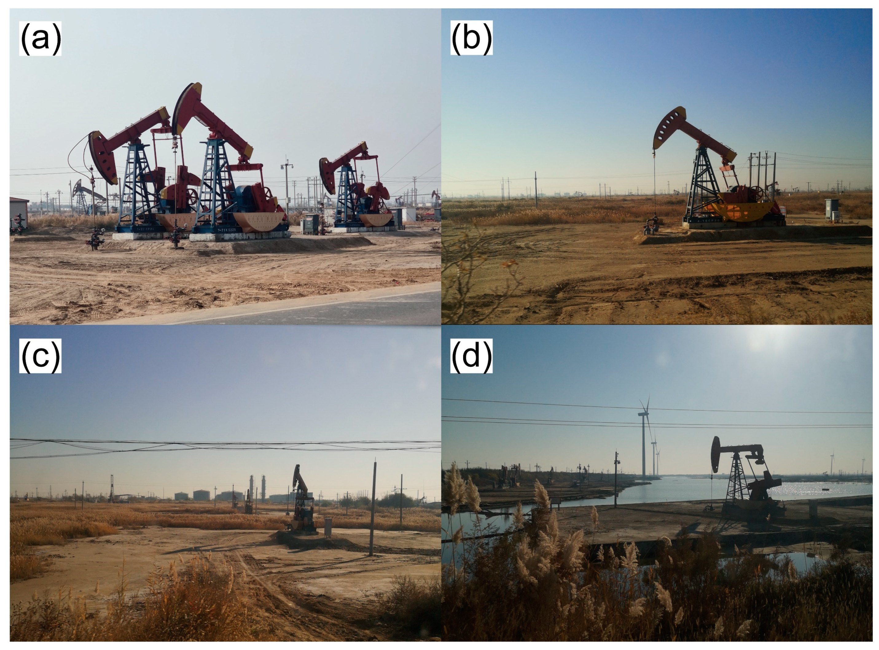
2.1. Study Area

The YRD (Figure 1) is located in the northeast of Dongying City, with Laizhou Bay to the east and Bohai Sea to the north; the area has a temperate continental monsoon climate. The YRD coastal wetlands are the most extensive, the most complete, and the youngest wetland ecosystem in China’s warm temperate zone, which has been included in the Ramsar Convention. In addition, it is also the wintering habitat for a concentrated distribution of rare and endangered birds [29]. The wetland vegetation is mainly aquatic and halophytic, whilst the soil types are mainly aquatic and salty soil. Every year, the Yellow River carries a large amount of sediment deposited at the mouth of the river, resulting in an increase in the estuarine silting land, and the estuary shoreline advances toward the Bohai Sea [26,30]. Therefore, it provides a large number of land resources for development and construction in the area, making it the most promising agricultural area in East China [31]. However, in the past 30 years, extensive human activities such as dam construction, oil and gas exploitation, groundwater pumping, agricultural irrigation, artificial diversion of the estuary, and artificial water-sediment regulation scheme [26,27,28,32] have posed serious threats to coastal wetlands in the YRD.

2.2. Datasets

In this study, we used 14 C-band Sentinel-1B (hereinafter referred to as S1B) images from 2019 to 2020, nine ALOS-2 PALSAR (hereinafter referred to as ALOS2) images, and one multispectral Sentinel-2A (hereinafter referred to as S2A) image. The data details are shown in

Table 1. SAR and optical remote sensing imagery used in this study.

Sensors	Acquisition Date (yyyy.mm.dd)	Imaging Mode	Resolution (m) (Range × Azimuth)	Polarization
Sentinel-1B (C-band SAR)	2019.02.28	IW (Interferometric wide swath)	2.3 × 14	VH + VV
	2019.03.24
	2019.04.29
	2019.05.23
	2019.06.16
	2019.07.10
	2019.08.03
	2019.08.27
	2019.09.20
	2019.10.26
	2019.11.19
	2019.12.25
	2020.01.06
ALOS-2 PALSAR (L-band SAR)	2014.12.06	Stripmap	4.3 × 3.4	HV + HH
	2015.07.18
	2015.09.26
	2015.10.24
	2016.07.16
	2016.12.03
	2017.03.25
	2018.11.03
	2019.05.18
Sentinel-2A (Optical)	2019.09.29	MSI (Multispectral instrument)	10 × 10	——

. After data preprocessing, we combined SAR backscattering intensity images, SAR interferometric coherence images, and optical images to obtain the following five datasets (Figure 2): optical data (hereinafter referred to as OPT); SAR backscattering intensity data (hereinafter referred to as PWR); optical and interferometric coherence image overlay data (hereinafter referred to as OPT + COH); SAR backscattering intensity and interferometric coherence image overlay data (hereinafter referred to as PWR + COH); and optical, radar backscattering intensity and coherence image overlay data (hereinafter referred to as OPT + COH +PWR), respectively.

The correlation coefficient images obtained through InSAR coherence processing were projected to the same coordinate system with the multispectral images and resampled to the same spatial resolution of 20 m. Then, the sample data of different land cover type were extracted from the region of interest (ROI). Next, the supervised classifiers (RF, NB, and MLP) were trained with the training set $T=\{(x_1,y_1),(x_2,y_2),\cdots ,(x_N,y_N)\}$. Finally, based on the original projection coordinate system, the predicted one-dimensional results were output as a classification image with geographic information.

Table 2. The number of classification training and validation samples per class.

Class	Training Samples (Pixel)	Validation Samples (Pixel)
Bare land	3429	1169
Building	3541	1201
Farm land	4587	1513
Grass	1950	631
Industrial land	2518	855
Mudflat	6570	2198
Saltpan	2445	804
Shrub	1317	523
Water	9902	3293
Total	36,259	12,187

lists the per-class numbers of training and validation samples (a total of 48,446 samples).

2.3. Methods

Figure 3 shows the main workflow of this study, including data preprocessing, image fusion, CCD, synergetic classification, and accuracy evaluation. First, the obtained Sentinel-1 SAR data and Sentinel-2 multispectral data were preprocessed with Sentinel Application Platform (SNAP) version 8.0.0 (https://step.esa.int, accessed on 1 March 2021), European Space Agency (ESA) and clipped to the range of the study area. Then, the processed optical images (OPT), SAR backscattering intensity images (PWR), and SAR coherence images (COH) were resampled to a uniform pixel size (20 m) and projection coordinate system (WGS84-UTM-50N). Secondly, training samples were extracted from stacking images through region of interest to train the three supervised classifiers with Python 3.9.0. The trained classifiers were applied to the classification of the whole study area to obtain the classification image, and then the accuracy of the results was evaluated. Meanwhile, the automatic threshold segmentation (OTSU) algorithm was used to divide the preprocessed coherence images into coherence changing and unchanging regions, and the annual variation characteristics of the coherence in the study area were obtained by time series analysis. Finally, the results of coherence change detection and synergetic classification were combined to obtain the coherence change characteristics and change areas of different land cover types in the study area.

2.3.1. Interferometric Coherence Processing

Two groups of waves in space that have the same wavelength or frequency and the same initial phase or the same phase difference are called coherent waves. Coherence refers to the phase similarity of coherent waves, and the result obtained through coherence calculation is the degree of similarity between two waves [33]. SAR interferometric coherence uses the principle of coherent waves to process two SAR images of the same scene collected at different times [34]. In SAR image processing, the similarity degree of two SAR images is represented by the coherence (complex correlation coefficient), and the theoretical model of coherence is shown in Equation (1) as follows:

$$\gamma =\frac{\mathrm{E}[u_1{u}_2^{*}]}{\sqrt{\mathrm{E}[{|u_1|}^2] \mathrm{E}[{|u_2|}^2]}}$$

(1)

where $\mathrm{E}[\cdot ]$ is the mathematical expectation; $u_1=|u_1|e^{j{\phi }_1}$ and $u_2=|u_2|e^{j{\phi }_2}$ are the primary and secondary image, respectively; and $u_2^{*}$ is the complex conjugate of $u_2$; ${\phi }_1$ and ${\phi }_2$ are the phase of the primary and secondary image, respectively.

In the remote sensing image processing, the correlation coefficient is generally estimated within the sliding window:

$$\widehat{\gamma }=\frac{{\displaystyle \sum _{n=1}^N{\displaystyle \sum _{m=1}^M{u}_1(n,m)u_2^{*}(n,m)}}}{\sqrt{{\displaystyle \sum _{n=1}^N{\displaystyle \sum _{m=1}^M{|u_1(n,m)|}^2{\displaystyle \sum _{n=1}^N{\displaystyle \sum _{m=1}^M{|u_2(n,m)|}^2}}}}}}$$

(2)

where N and M are the size of sliding window for the primary and secondary images, respectively, while n and m represent the row and column indices within the window.

The value of the coherence is distributed within [0, 1]. The closer the coherence approaches to 1, the more similar the corresponding homonymous image point is, indicating that the ground object does not change during the imaging period. When the coherence is closer to 0, the ground objects have changed during the imaging period [35]. In general, the coherence will decrease with an increase in spatiotemporal baselines between the primary and secondary images [19].

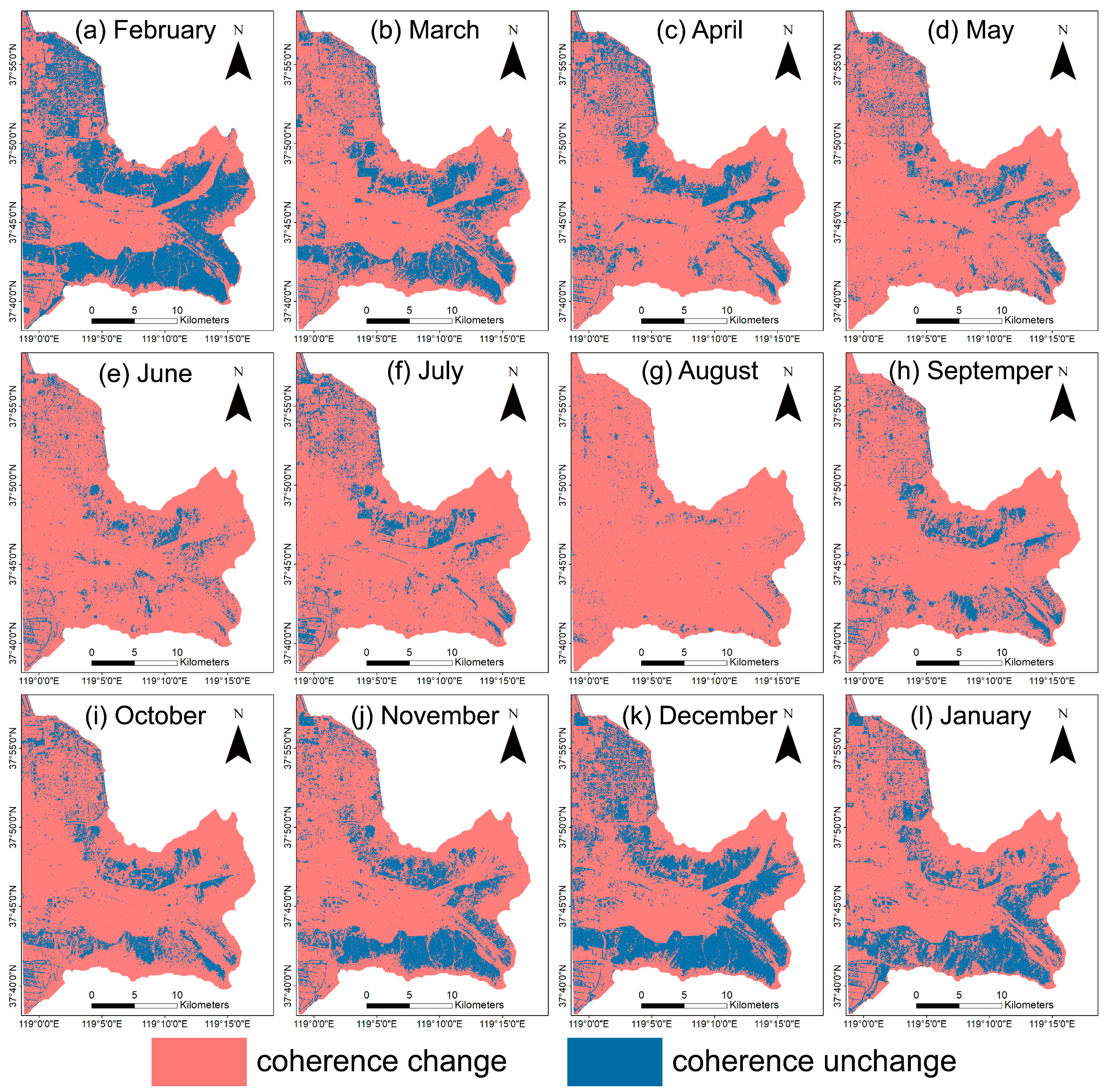
2.3.2. Coherence Change Detection

Image segmentation is a method that divides a digital image into several groups of pixels, whose main purpose is to simplify the image and make it easy to analyze [36]. Considering the influence of the intensity difference between target and background and the size of target, the maximum inter-class difference threshold segmentation (OTSU) algorithm has been widely used in image segmentation due to its advantages of simple calculation and being independent of the position of the target in an image [37]. Therefore, the OTSU algorithm was used to segment and binarize the images, reduce the amount of data, and highlight the coherence changing area contour.

Mathematical morphology based on topology and lattice theory is used for image processing and analysis. The basic operations are erosion and dilation algorithms that are realized by a sliding window convolution operation on the target image to calculate the window minimum (erosion) value or maximum (dilation) value. Then, the minimum value or maximum value is assigned to the specified pixel of the reference point so that it will gradually decrease (erosion) or expand the highlighted area (dilation) of the image. Open and close operations are combined operations based on erosion and dilation operations. The open operation, first, erodes the image, and then expands the results of the erosion, which can be used to smooth the contour, disconnect the narrow connection, and eliminate the sharp protruding part of the edge. In the close operation, the image is first dilated, and then eroded, which is used to bridge narrow discontinuities and slender gully, eliminate small holes, and fill contour fracture [38].

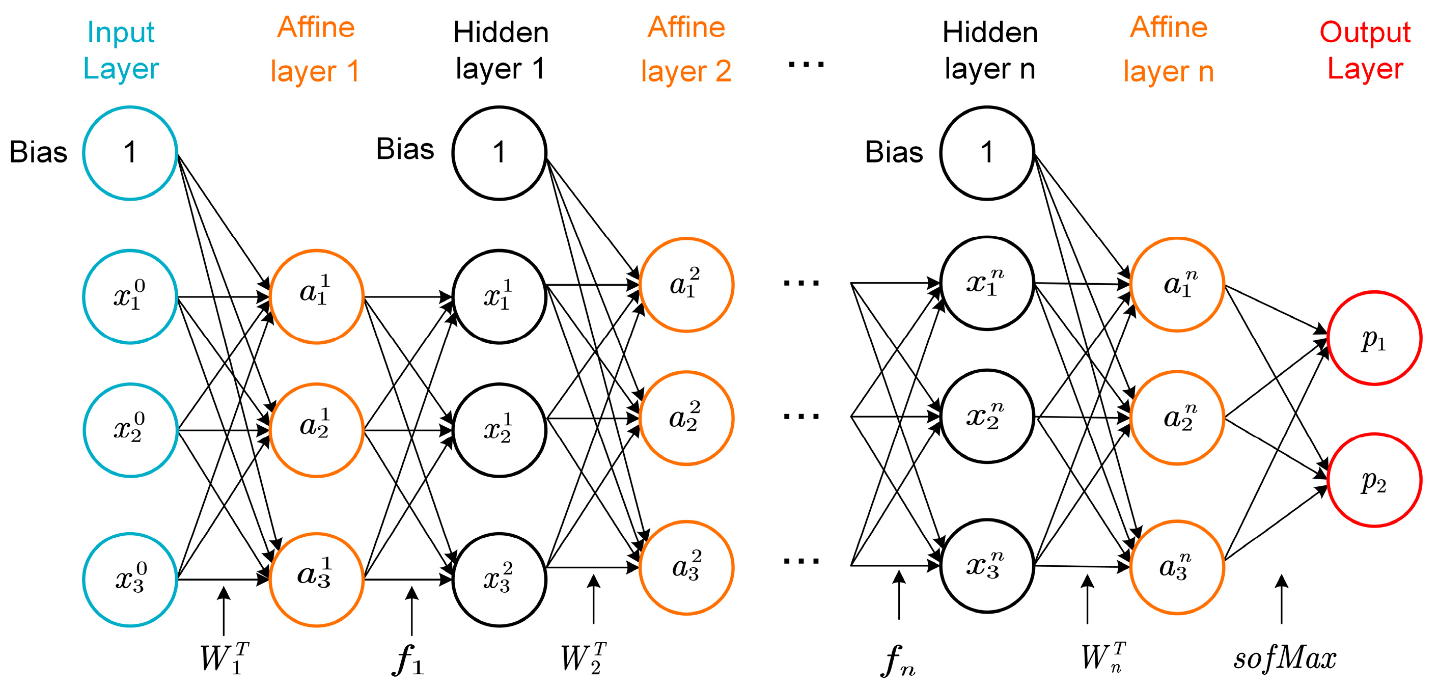
2.3.3. Supervised Classification

In this study, three classical machine learning algorithms, that is, naive Bayes (NB), random forest (RF), and multilayer perceptron (MLP), were used for synergetic classification of features from multispectral images, multi-band SAR backscatter intensity images, and coherence images.

The NB algorithm is developed based on Bayesian theory [39]:

$$\mathrm{P}(y_i|x)=\frac{\mathrm{P}(x|y_i) \mathrm{P}(y_i)}{\mathrm{P}(x)}$$

(3)

where $y_i\in \{y_1,y_2,\dots ,y_K\}$ is the $K$ possible category tags and $x=(x_1, x_2, x_3, \dots , x_n), x\in {ℝ}^n$ is the multidimensional random variable.

Given an event $x$, its probability distribution of $\mathrm{P}(x)$ is certain, and $\mathrm{P}(y_i)$ is called the prior probability of an event, while $\mathrm{P}(y_i|x)$ is the posteriori probability. The attribute conditional independence assumption of naive Bayesian theory means that each feature of a multidimensional random variable is independent of the other (Equation (4)):

$$\mathrm{P}(x|y_i)=\mathrm{P}(x_1,\dots ,x_n|y_i)={\displaystyle \prod _{j=1}^n\mathrm{P}(x_j|y_i)}$$

(4)

where n is the number of feature categories, and $x_j$ is the value of $x$ on the jth attribute.

Because the $\mathrm{P}(x)$ is a constant relative to the input data, it can be removed. Now, we need to build a classification model to calculate the probability with all possible values of the known class variables, and select the result with the maximum probability as the output (Equation (5)):

$$\widehat{y}=\underset{y_i}{\arg \max }\mathrm{P}(y_i){\displaystyle \prod _{j=1}^n\mathrm{P}(x_j|y_i)}$$

(5)

RF is a non-parametric ensemble classifier, which is independent of input data distribution and can effectively adapt to input data with a large number of different types and scales. Due to its high robustness to noise and overfitting [40], it has attracted more and more attention. The classification results of RF are determined by all decision tree voting. Each decision tree is generated by random sampling from the training set by the bootstrap sampling strategy. Meanwhile, the generalization ability of RF can be enhanced by adjusting the number of decision trees (Ntree) and the number of variables (Mtry), to finally achieve the classification purpose [41].

An MLP, also known as an artificial neural network (ANN), includes an input layer, a hidden layer, and an output layer (Figure 4). The simplest MLP contains only one hidden layer [42]. The input layer $x\in {ℝ}^n$ is mapped to the affine layer by linear transformation:

$$a(x)={\omega }^{\mathrm{T}}x+b$$

(6)

where the ${\omega }^{\mathrm{T}}$ is the weight vector, and the $b$ is bias. Then, the affine layer is mapped to the hidden layer by the nonlinear sigmoid function:

$$f(x)=\frac{1}{1+e^{-a(x)}}$$

(7)

where the $a(x)$ is the output of the affine layer. The affine layer and nonlinear layer propagate forward alternately and finally generate the output layer by softmax function. When each feature of the latter layer is obtained by all the features of the previous layer, it is called fully connect [43].

2.3.4. Accuracy Assessment

A confusion matrix is employed to provide a basis for other metrics to quantitatively evaluate classification accuracy.

Table 3. The confusion matrix for a binary classification problem.

	Predicted Label	Positive	Negative
Real Label
Positive		TP	FN
Negative		FP	TN

shows a simple model of the confusion matrix, where the positive and negative values are the categories of the two classes. True positive (TP) indicates that the sample real label is positive and the predicted label is also positive. False positive (FP) indicates that the sample real label is negative but the predicted label is positive. True negative (TN) indicates that the sample real label is negative and the predicted label is also negative. False negative (FN) indicates that the sample real label is positive but the predicted label is negative. To evaluate the performances of the three classifiers, four important metrics (recall, precision, accuracy, and F1 score) are illustrated and described below. The F1 score, which weights precision and recall equally, is the variant most often used to provide a better assessment of model performance when learning from imbalanced data.

(i)

Recall

Recall indicates the proportion of positive samples correctly predicted to all real positive samples, which is used to evaluate the detection coverage of the classifier for all targets to be detected. The formula for the recall is expressed as follows:

$$Recall=\frac{TP}{TP+FN}$$

(8)

(ii)

Precision

Precision indicates the proportion of true positive samples to all predicted positive samples, which is used to evaluate the correctness of the classifier given successful detection. The formula for the precision is expressed as follows:

$$Precision=\frac{TP}{TP+FP}$$

(9)

(iii)

Accuracy

Accuracy indicates the proportion of samples correctly classified by the model to the total samples. The formula for the accuracy is expressed as follows:

$$Accuracy=\frac{TP+TN}{TP+TN+FP+FN}$$

(10)

• (iv) F1 Score

The F1 score takes into account both the recall and precision of the classification model and can be considered to be the weighted average of the recall and precision of the model. The F1 score has a value range from 0 to 1, and a larger value indicates a better model, as shown in the following formula:

$$F1 score=\frac{2\ast Precision\ast Recall}{Precision+Recall}$$

(11)

3. Results

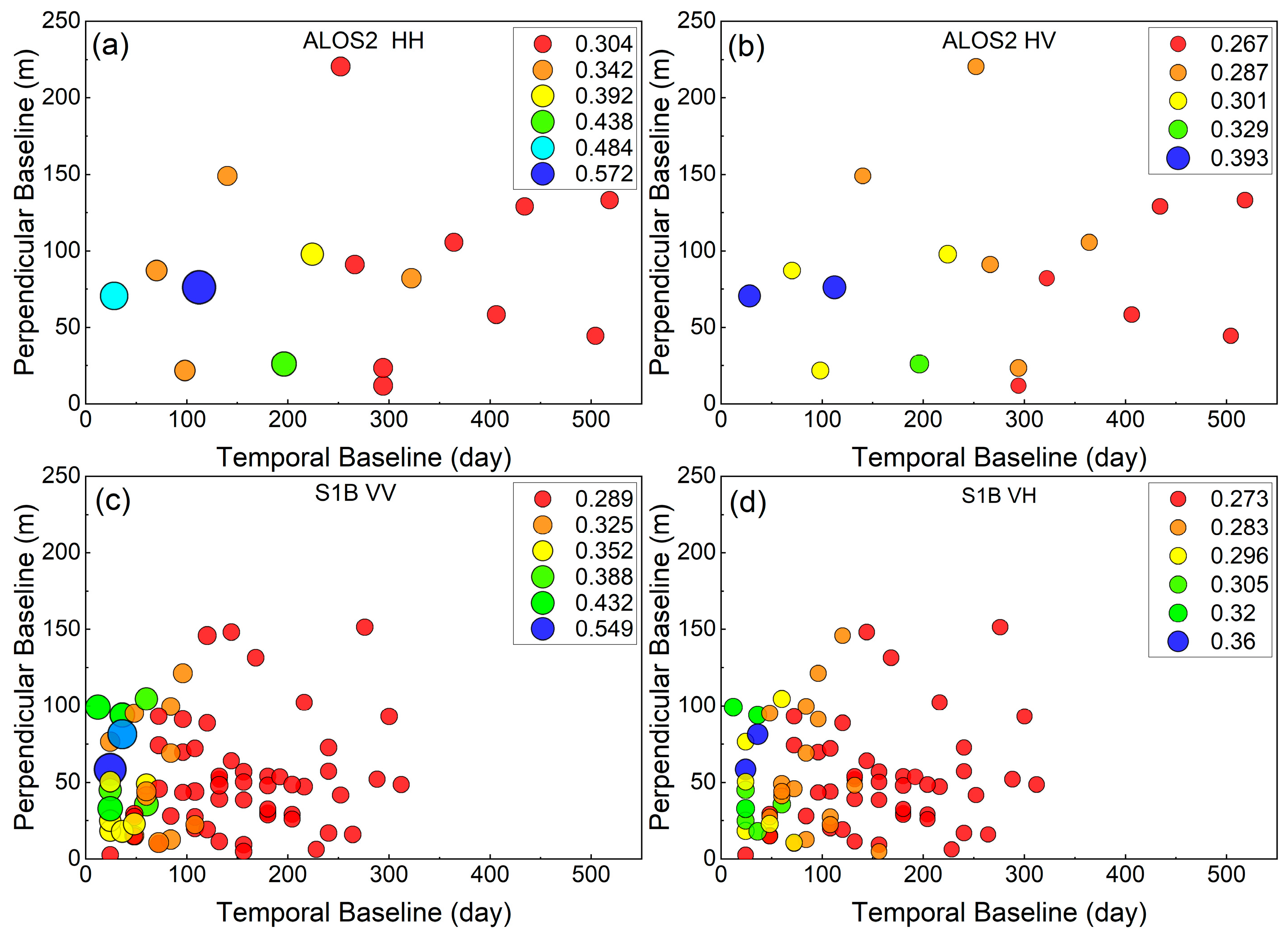
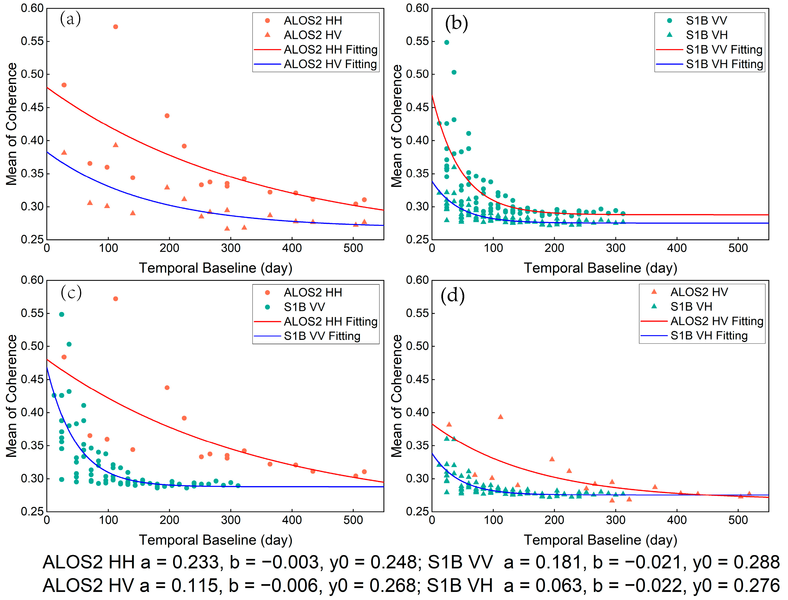
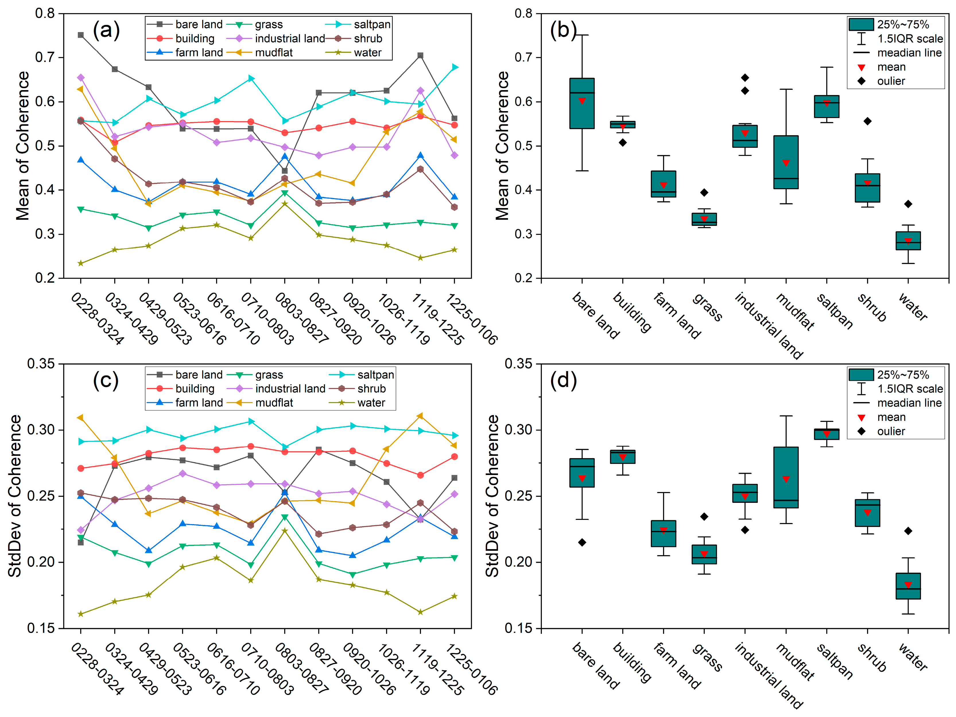
3.1. Coherence Comparison

X-band satellites are easily affected by dense vegetation, resulting in poor coherence. Therefore, in this study, we chose to analyze the C-band S1B and L-band ALOS2 images. Figure 5 depicts the interferometric coherence of L-band ALOS2 from 17 interferograms and C-band S1B from 77 interferograms as a function of the temporal baseline and perpendicular baselines. As seen, the interferometric coherence of the ALOS2 and S1B is greatly affected by the temporal baseline, especially for the S1B with short wavelength. For example, the mean coherence of ALOS2 remained above 0.35 within 100 days, while that of S1B dropped to about 0.28. On the contrary, the interferometric coherence appears to be less affected by the perpendicular baseline within 250 m. Therefore, the interferometric coherence as a function of the temporal baseline can be fitted into the exponential descent function $y=a\times {\mathrm{e}}^{bx}+y_0$ with 95% confidence bounds.

Figure 6 shows the fitting curves in different polarization modes of ALOS2 and S1B. As shown in Figure 6a,b, interferometric coherence in co-polarization mode (HH and VV) is generally greater than that in cross-polarization mode (HV and VH). Meanwhile, as the temporal baseline increases, the fitting curves in co-polarization mode decline slightly faster than that in cross-polarization mode. Figure 6c,d depict that the interferometric coherence of ALOS2 is almost higher than that of S1B regardless of co-polarization mode or cross-polarization mode within 300 days. In addition, as the temporal baseline increases, the S1B interferometric coherence fitting curve decreases faster than that of ALOS2 within 100 days. However, in the case of a short temporal baseline (12–24 days), the interferometric coherence of S1B has stably distributed between 0.35 and 0.45, and even some data has exceeded ALOS2 in the co-polarization mode. This indicated that the C-band SAR with a short temporal baseline can be used for the coherence change detection in coastal wetlands.

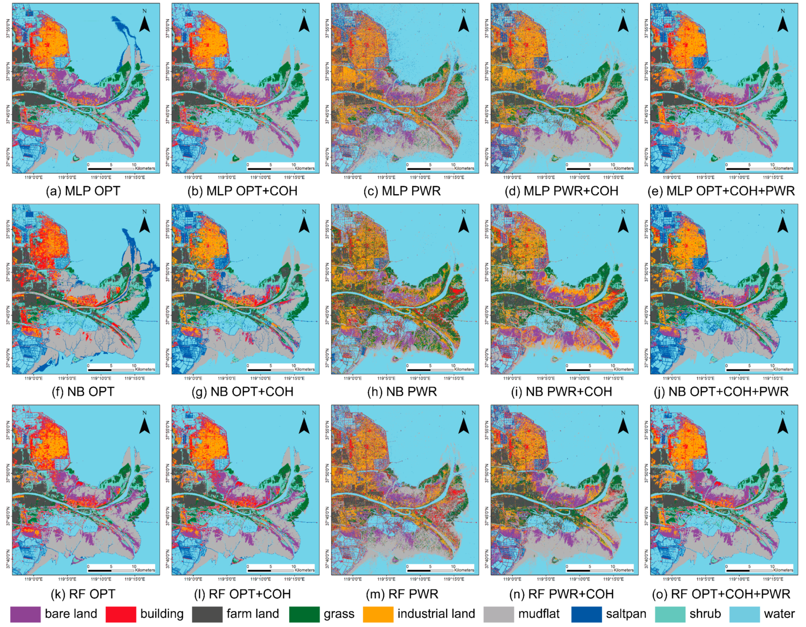
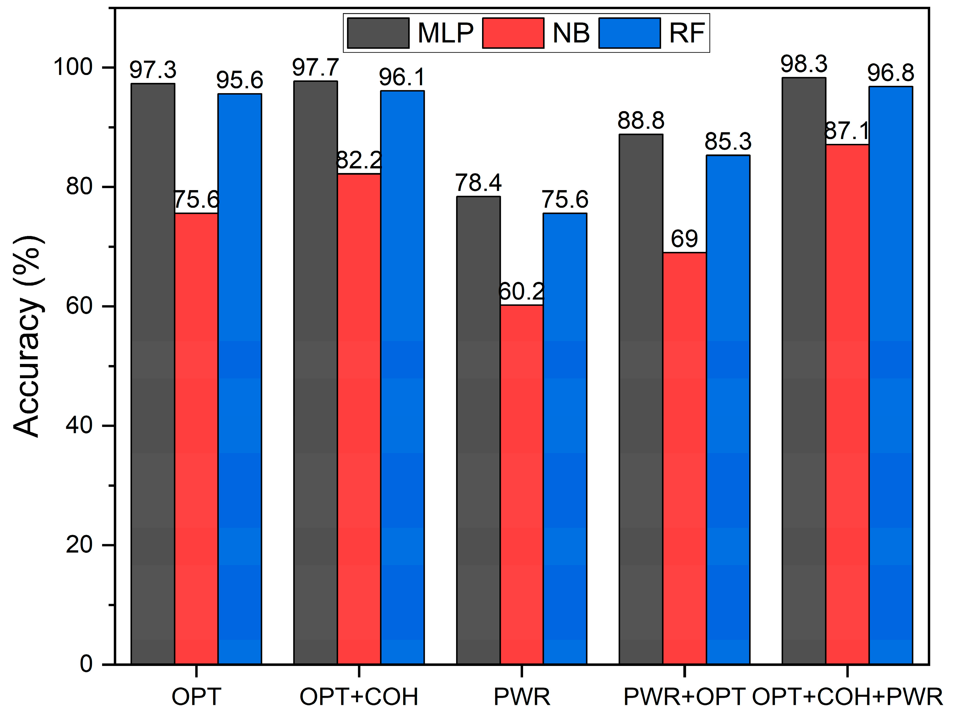
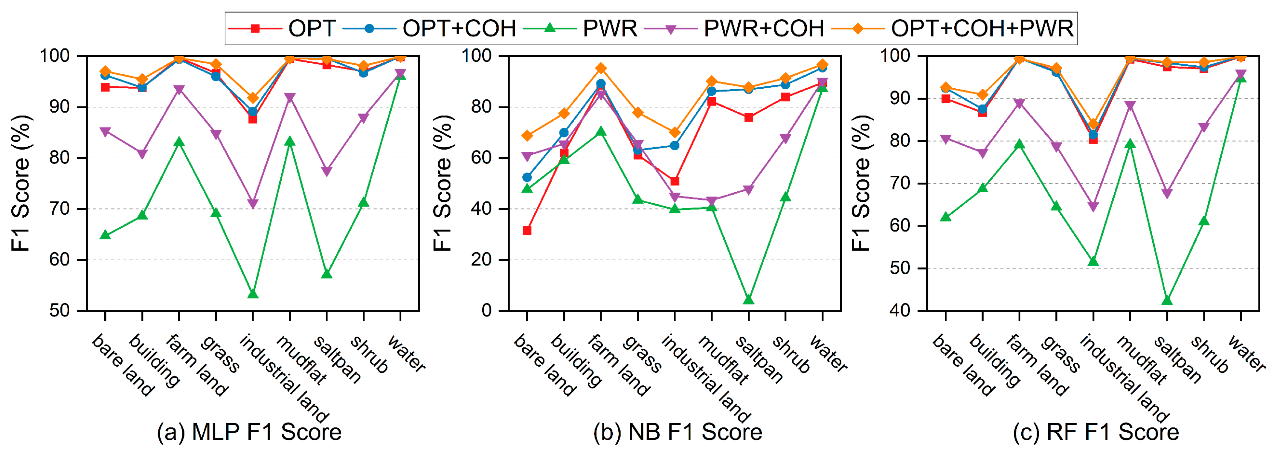
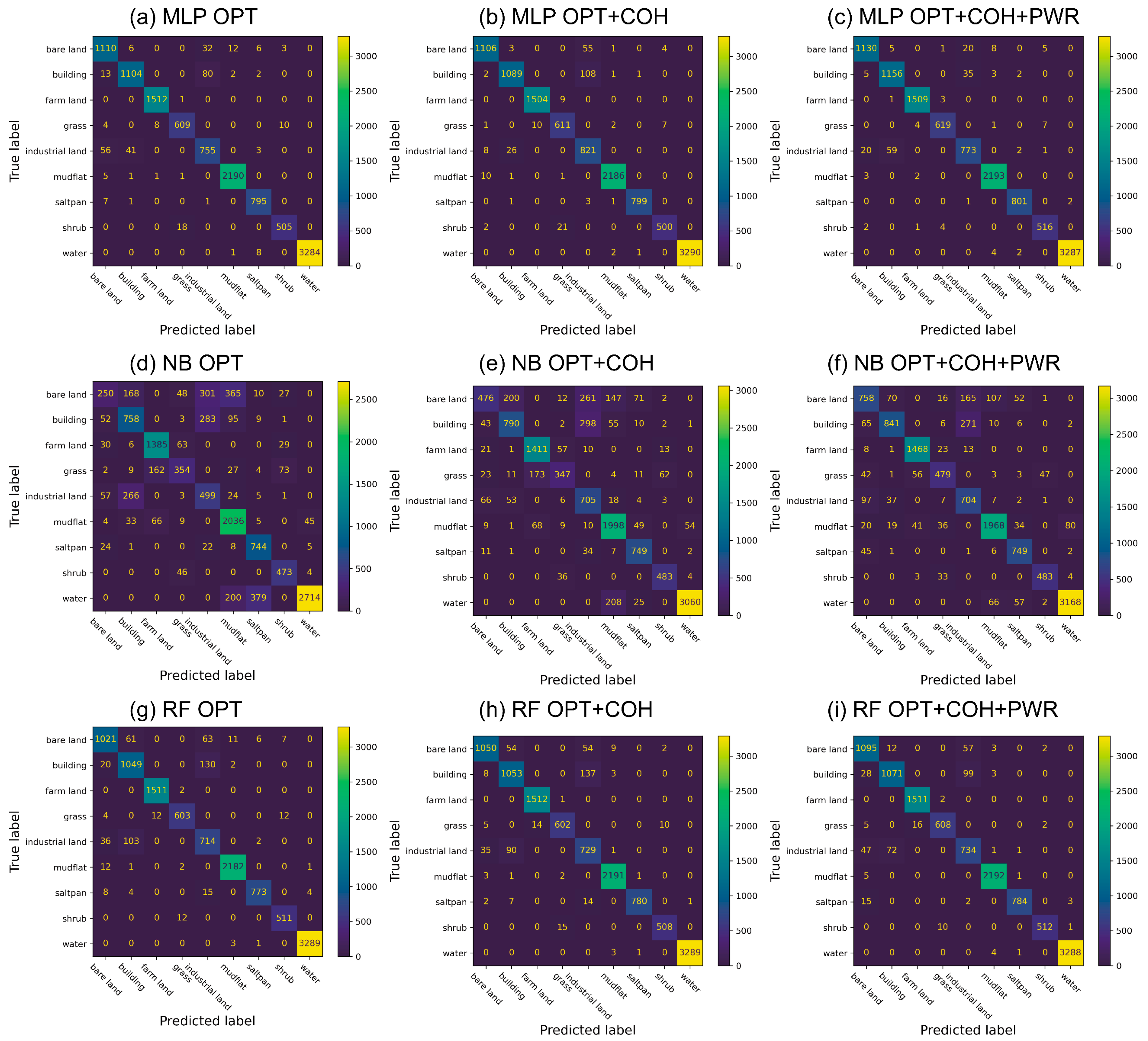
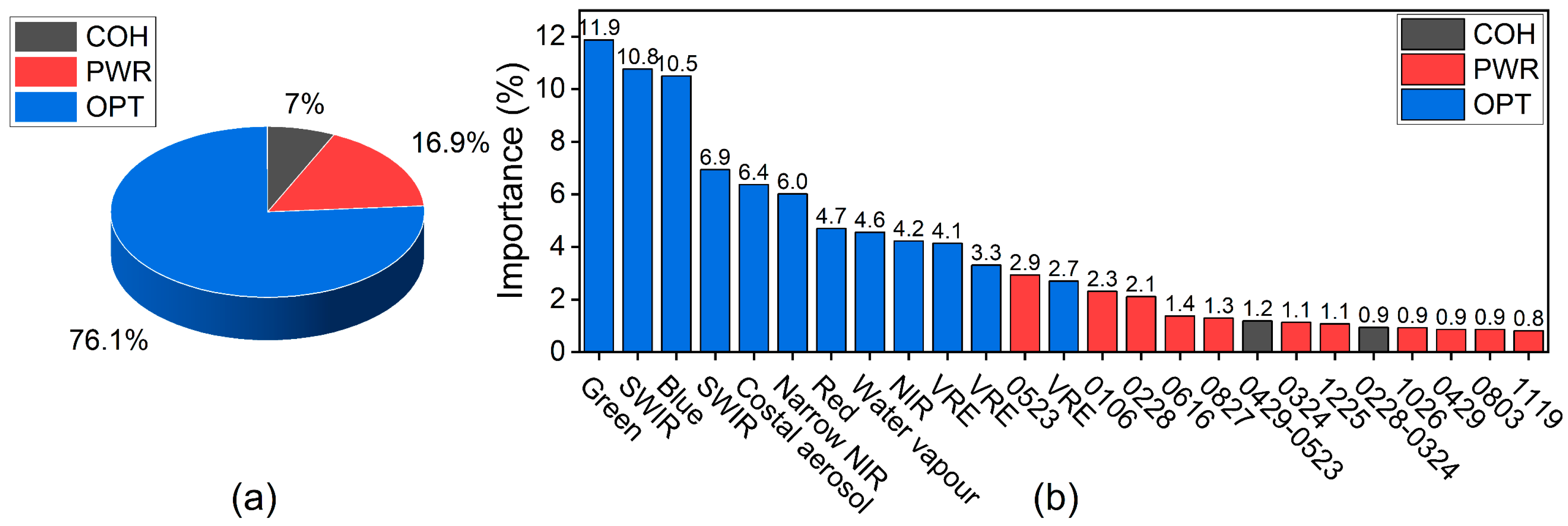
3.2. Synergetic Classification

In this section, we use 12 Sentinel-1 InSAR coherence images, 13 Sentinel-1 SAR backscattering intensity images, and one 12-bands atmospherically corrected Sentinel-2 Level-2A MSI orthoimage for synergetic classification. In fact, two Sentinel-2 satellites can be revisited every five days under cloud-free conditions. Since a fixed Sentinel-2 image as input data is required to avoid the influence of irrelevant variables on the evaluation of coherence change detection, we did not use all available Sentinel-2 MSI images.

Figure 7 presents the classification maps derived from MLP, NB, and RF methods for the OPT, OPT + COH, PWR, PWR + COH, and OPT + COH + PWR datasets. The results for the datasets containing multispectral images (OPT, OPT + COH, andOPT + COH + PWR) show that each land cover type is relatively complete and the boundary between different land cover types is clear, whereas the severe pepper noise in radar images results in poor integrity of land cover in classification results (PWR and PWR + COH). However, there are a lot of misclassification results when only using multispectral images to classify in the study area, such as the misclassification of saltpan in the estuary (Figure 7a,f), while the result of synergetic classification effectively alleviates the misclassification of salt pans (Figure 7b,g). This indicates that the synergetic classification method makes up for the deficiency of multispectral image in classification, but also greatly restrains the influence of SAR pepper noise on the classification result.

Figure 8 shows the classification accuracy of three classification methods for five different datasets. Firstly, since the PWR data have the lowest accuracy, single PWR data are not suitable for accurate classification. Secondly, the accuracy of the OPT + COH + PWR data is the highest in the five different datasets for any of the three classification methods. Third, among the three classifiers, the MLP classifier performs best (98.3%), whilst the NB classifier has the lowest accuracy, and the accuracy of the RF classifier differs from that of MLP by about 2%. Fourth, the accuracies of the three methods in the PWR + COH data are all improved about 10% higher than that in PWR. Finally, the accuracy of the MLP and RF methods in the OPT + COH data is slightly higher than that in the OPT data, whilst the accuracy of the NB method can be improved 6.6%. Therefore, we are confident that SAR coherence can be used as an effective feature to participate in synergetic classification and improve the overall accuracy.

Although it has been proved that coherence-based synergetic classification can improve accuracy, an improvement in diverse land cover is different. Figure 9 demonstrates the F1 score of classification for nine different land cover types. First, it shows that coherence images (COH) contribute to the synergetic classification. The F1 scores of the nine land cover types in the synergetic classification result (OPT + COH and PWR + COH datasets) for all three classification methods (MLP, NB, and RF) are slightly improved as compared with single data sources (OPT and PWR datasets). The F1 scores of the PWR + COH data are higher than that of the PWR data by about 10% in nine land cover types except for water, while the F1 scores of the OPT + COH data are slightly improved as compared with that of the OPT data. Meanwhile, the F1 scores of the OPT + COH + PWR data are almost the highest in the five different datasets for the three supervised methods. Secondly, the contribution of coherence to the synergetic classification of bare land, building, saltpan, and industrial land in SAR data is higher than that of other land cover types. In addition, it also shows that the F1 score of industrial land is almost the lowest in all five datasets, which is probably attributed to the complex land surface characteristics in the oilfield.

The F1 score reflects the comprehensive classification accuracy level of different land covers, whilst the confusion matrix can show the misclassification details more clearly. For examples, the industrial land is mainly misclassified as building and bare land by the three classifiers (MLP, NB, and RF), while the bare land and building are also mainly misclassified as the industrial land (Figure 10). It indicates that the features of industrial land are similar to other land covers, which leads to misclassification to a large extent.

The spatial resolution of multi-source remote sensing images represents the ability to detect the details of coastal wetlands. For features less than 20 m, such as drilling platforms, buildings, artificial objects, small shrubs, etc., they are usually mixed together, which may lead to the uncertainty of synergetic classification. Figure 11 shows the pumping units are very common in the industrial land of the YRD. As the China’s second largest oilfield, the Shengli oilfield is located on both sides of the Yellow River estuary and covers an area of 44,000 square kilometers. The pumping unit has a vertical angle to the ground, producing a strong corner reflector effect like a building in SAR images, surrounded by bare land, which makes it prone to be misclassified as building and bare land. However, the misclassification of industrial land with SAR data can be effectively alleviated with OPT + COH + PWR data, thus the number of correctly classified pixels increases.

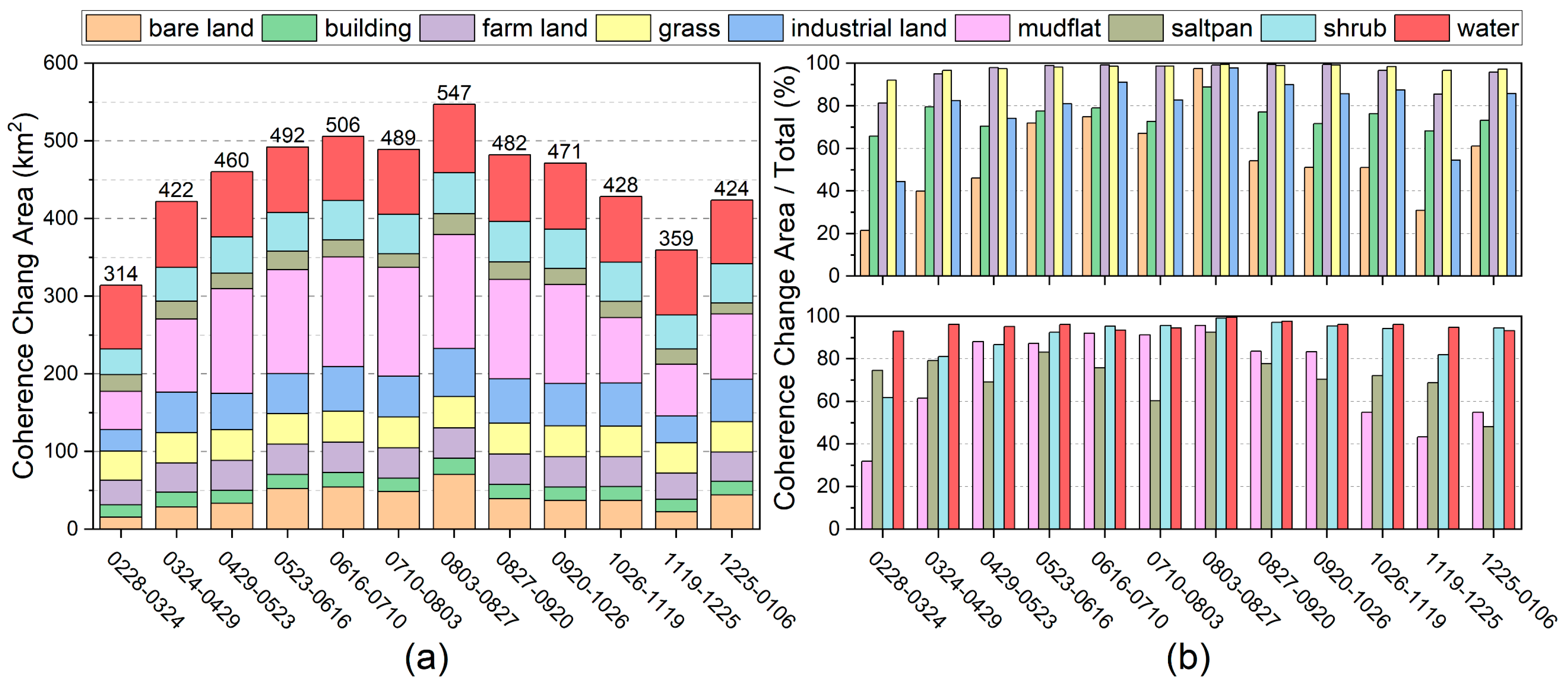
3.3. Coherence Change Area

Figure 12 shows the results of CCD in the YRD throughout the whole year 2019. First of all, the regions with coherence change and unchanged have a strong spatiotemporal correlation in the study area. The areas of coherence change are mainly distributed in the coastal areas on both sides of the estuary, wetlands in the middle of the study area and farm land. However, the areas of coherence unchanged are mainly located in the oilfield area in the northwest of the study area, the bare land and the part of mudflat above the high-water line. Secondly, the range of coherence changed region generally increases from spring (March to May) to summer (Jun to August), and decreases from autumn (September to November) to winter (December to February). August has the largest coherence change area, almost covering the whole study area, while the smallest in February.

In order to analyze the correlation between coherence change and land cover, we separate the coherence change regions into different land cover types (Figure 7e) and different months and calculate their areas (Figure 13). Firstly, we can see a quantitative description of the area of coherence changes over the YRD, in which it increases from spring to summer and decreases from autumn to winter (Figure 13a). February has the lowest change area (314 km²), while August has the annual maximum of coherence change area (547 km²). Secondly, the coherence change area for each month is more than 60% of the total land area (565 km²) except for February. In addition, the coherence change area is mainly composed of mudflat, water, followed by bare land, farmland, grass, industrial land and shrub, whilst building and saltpan account for the least proportion. Assumed that the classified areas of various land covers remain relatively stable throughout the year, Figure 13b depicts the proportion of the coherence change area for each land cover to the total area of the land cover type in each month. Among them, the proportion of coherence change area in water and grass remained above 90% throughout the year, whilst bare land has the lowest proportion of 20% in February.

4. Discussion

4.1. Interferometric Coherence Analysis

The result in Figure 5 indicates that the temporal baseline has a greater impact on the interferometric coherence than the perpendicular baseline. Because present-day SAR satellites have relative strict orbital control, the perpendicular baselines between the primary and secondary images are generally not large, which can also be seen from Figure 5 that the perpendicular baselines are controlled within 250 m. Furthermore, by comparing Figure 6c with Figure 6d, it can be seen that SAR images with a longer wavelength can obtain a higher interferometric coherence for a longer temporal baseline, which is consistent with previous studies [21]. This is attributed to the reason that the shorter-wavelength C-band has a shallower penetration depth than the L-band and mainly interacts with the upper canopy that is susceptible to environmental influences such as wind. Therefore, C-band SAR signals lose consistency over a long period [44]. Although the C-band decays faster as the temporal baseline increases than that of the L-band in the fitting function of interferometric coherence, the C-band SAR in a short temporal baseline can maintain coherence stability, which can be used to analyze the coherence changes in coastal wetlands. Therefore, the SAR interferometric coherence can reflect the changing information of the ground surface, which can be used to provide reliable data sources for the examination of coastal changes.

An InSAR coherence image is a cross-correlation product of two complex numerical SAR images, which describes the change of the backscattering characteristics on the radar wavelength scale, also expressed as the degree of similarity between two pixels. The loss of InSAR coherence is often referred to as decorrelation, which includes several reasons, such as volume decorrelation caused by volume backscattering effect, temporal decorrelation caused by the change of environment over time, geometric decorrelation from different radar viewing angles, and thermal noise decorrelation from radar instruments. In addition, SAR image registration errors and other InSAR processing errors can also reduce InSAR coherence levels. For Sentinel-1 IWS data, very strict (~1/1000 pixel) azimuth registration is required, otherwise there will be significant phase jumps between bursts. The accurate registration with enhanced spectral diversity (ESD) can effectively estimate the residual azimuthal offset in the overlapping region, and ensure the final registration accuracy of Sentinel-1.

4.2. Synergetic Classification Accuracy

Comparing the classification methods (MLP, NB, and RF) for different datasets (Figure 8), the classification accuracy with the fusion datasets (OPT + COH and PWR + COH) are higher than that of the single dataset (OPT or PWR). It proves that the synergetic classification with coherence images can effectively improve the classification accuracy. Meanwhile, the accuracy of classification with OPT + COH + PWR data is almost the highest in five different datasets, which indicates that the synergetic classification with multispectral feature, SAR coherence and intensity has great advantages in coastal wetland areas with dense vegetation and changeable weather. As shown in Figure 9, the F1 scores of different land covers vary greatly where the F1 scores of bare land, building, and industrial land are lower than those of other land covers. In addition, the method of synergetic classification can significantly improve the F1 scores of most land covers except for industrial land.

Figure 14 shows the importance of different bands in OPT + COH + PWR datasets to classification results of RF classifier. Firstly, the OPT multispectral data accounts for three quarters of the RF classification contribution, while SAR data accounts for about a quarter (Figure 14a). It indicates that fusion of SAR intensity (PWR) and coherence (COH) can provide valuable information for classification of costal wetland [20,45]. Although backscatter intensity has higher availability compared to the coherence [44], datasets that combines both coherence and intensity are superior to either data alone [9]. Secondly, among the most important 25 bands for synergetic classification (Figure 14b), the OPT data occupies 11 bands, where the green band is the most important (11.9%) in all bands. In addition, the PWR data occupies 11 bands, while the COH data occupies two bands and the classification importance is lower than the PWR and OPT datasets. However, coherence change feature still has abundant complementary information for coastal wetland classification [24].

Since SAR coherence can be used as an important index for coastal wetland change detection, the synergetic classification accuracy can be significantly improved by integrating the SAR coherence, SAR intensity and multispectral remote sensing images. However, it should be noted that the multispectral images contribute the most important spectral features and texture features required for synergetic classification. In addition, SAR backscattering intensity of a ground target is a function of SAR wavelength, image acquisition geometry, local topography, surface roughness, and the permittivity of the target, which also depends on vegetation height, biomass, density, and flood conditions of the coastal wetlands. Therefore, the classification results using coherence alone may not outperform multispectral data or SAR intensity data to some extent, especially in the complex coastal areas.

4.3. Driving Factors of Coherence Change

Figure 15 depicts the coherence mean and standard deviation values of nine land cover types in different months in 2019. First, building and industrial land with strong backscattering usually maintaines a high and stable coherence mean (0.5~0.6) and standard deviation (0.25~0.3) throughout the year, indicating stronger conditions of interferometry and smaller activities for long periods (Figure 15a,c). Secondly, water body mostly due to specular reflection has the lowest coherence mean (0.2~0.4) and standard deviation (0.15~0.2) among all the land cover types, which indicates a poor interferometry condition and is consistent with the actual situation. Third, mudflat and bare land have relatively high coherence means (0.4~0.7) and standard deviations (0.2~0.3), which means that both of them change dramatically in different months. However, their opposite trend of standard deviation of coherence can probably be attributed to a change in soil moisture as a result of seasonal precipitation and storm surge [27,46], which directly leads to changes in their coherences. Therefore, the difference of standard deviation of coherence between bare land and mudflat can be used as a factor to distinguish the two kinds of land cover.

The differences between the upper and lower quartiles of the coherence mean and standard deviation in all land cover types remained at 0.05~0.1, except for bare land and mudflat (Figure 15b,d). This indicates that the coherence means and standard deviations of most land cover types remain relatively stable from month to month. In addition, both the medians of coherence mean (0.6) and standard deviation (0.3) in the saltpan are almost the highest among all the land cover types. This is mainly attributed to the seasonal brine extraction and salt extraction process, but may also be influenced by the grid of concrete pavement and large wind turbines in areas within the saltpan (Figure 1g and Figure 11d).

5. Conclusions

In this study, C-band Sentinel-1 and L-band ALOS-2 PALSAR data were used to detect spatiotemporal distribution and the change pattern of interferometric coherence in the coastal wetlands of the YRD. The interferometric coherence, as a function of temporal and perpendicular baselines, was mainly dependent on the former, while it was less affected by the latter, especially for shorter wavelengths. Then, the interferometric coherence as a function of the temporal baseline was fitted into the exponential descent function. The fitting curves indicate that interferometric coherence in co-polarization mode is generally greater than that of cross-polarization mode. Long wavelength SAR images can maintain higher coherences with long temporal baselines, whilst short wavelength SAR images also have high coherences with short temporal baselines.

Furthermore, we chose C-band S1B images in 2019 to reveal coherence changes in the YRD. The coherence change results shows that the OTSU algorithm can accurately extract the boundary of the coherence change region and obtain the annual coherence change characteristics with long-term observations. Overall, above 60% of the study area throughout the year is the coherence change region, except for February. The minimum (314 km²) and maximum (547 km²) coherence change occurred in February and August, respectively.

In addition, we proposed a method of synergetic classification with SAR coherence, intensity, and optical images for coastal wetlands. The correlation between coherence change and land cover is beneficial for coastal wetland mapping, which has proved to guide multisource data fusion to improve classification accuracy.

In general, the method of SAR coherence-based change detection and synergetic classification in this study can accurately extract and monitor the changing region and significantly improve the classification accuracy of complex coastal wetlands. In the context of the combined influence of global change and human activities, we have provided an alternative cost-effective method for coastal wetland change detection, which contributes to more accurate dynamic land cover classification and to an understanding of the response mechanism of land features to climate change and human activities.

References

1. Tiner, R.W.; Lang, M.W.; Klemas, V. (Eds.) Remote Sensing of Wetlands: Applications and Advances, 1st ed.; CRC Press: Boca Raton, FL, USA, 2015; pp. 119–136. [Google Scholar]
2. Vymazal, J. Constructed Wetlands for Wastewater Treatment. Water 2010, 2, 530–549. [Google Scholar] [CrossRef] [Green Version]
3. Gedan, K.B.; Kirwan, M.L.; Wolanski, E.; Barbier, E.B.; Silliman, B.R. The present and future role of coastal wetland vegetation in protecting shorelines: Answering recent challenges to the paradigm. Clim. Change 2011, 106, 7–29. [Google Scholar] [CrossRef]
4. Murray, N.J.; Phinn, S.R.; DeWitt, M.; Ferrari, R.; Johnston, R.; Lyons, M.B.; Clinton, N.; Thau, D.; Fuller, R.A. The global distribution and trajectory of tidal flats. Nature 2019, 565, 222–225. [Google Scholar] [CrossRef] [PubMed]
5. Prigent, C.; Papa, F.; Aires, F.; Jimenez, C.; Rossow, W.B.; Matthews, E. Changes in land surface water dynamics since the 1990s and relation to population pressure. Geophys. Res. Lett. 2012, 39, L08403. [Google Scholar] [CrossRef] [Green Version]
6. Junk, W.J.; Piedade, M.T.F.; Lourival, R.; Wittmann, F.; Kandus, P.; Lacerda, L.D.; Bozelli, R.L.; Esteves, F.d.A.; Nunes da Cunha, C.; Maltchik, L. Brazilian wetlands: Their definition, delineation, and classification for research, sustainable management, and protection. Aquat. Conserv. Mar. Freshw. Ecosyst. 2014, 24, 5–22. [Google Scholar] [CrossRef]
7. Wdowinski, S.; Kim, S.-W.; Amelung, F.; Dixon, T.H.; Miralles-Wilhelm, F.; Sonenshein, R. Space-Based detection of wetlands’ surface water level changes from L-band SAR interferometry. Remote Sens. Environ. 2008, 112, 681–696. [Google Scholar] [CrossRef]
8. Liao, T.-H.; Simard, M.; Denbina, M.; Lamb, M.P. Monitoring Water Level Change and Seasonal Vegetation Change in the Coastal Wetlands of Louisiana Using L-Band Time-Series. Remote Sens. 2020, 12, 2351. [Google Scholar] [CrossRef]
9. Brisco, B.; Ahern, F.; Murnaghan, K.; White, L.; Canisus, F.; Lancaster, P. Seasonal Change in Wetland Coherence as an Aid to Wetland Monitoring. Remote Sens. 2017, 9, 158. [Google Scholar] [CrossRef] [Green Version]
10. Mahdianpari, M.; Salehi, B.; Mohammadimanesh, F.; Brisco, B.; Mahdavi, S.; Amani, M.; Granger, J.E. Fisher Linear Discriminant Analysis of coherency matrix for wetland classification using PolSAR imagery. Remote Sens. Environ. 2018, 206, 300–317. [Google Scholar] [CrossRef]
11. Ramsey, E.W. Monitoring flooding in coastal wetlands by using radar imagery and ground-based measurements. Int. J. Remote Sens. 1995, 16, 2495–2502. [Google Scholar] [CrossRef]
12. White, L.; Brisco, B.; Pregitzer, M.; Tedford, B.; Boychuk, L. RADARSAT-2 Beam Mode Selection for Surface Water and Flooded Vegetation Mapping. Can. J. Remote Sens. 2014, 40, 135–151. [Google Scholar] [CrossRef]
13. Töyrä, J.; Pietroniro, A. Towards operational monitoring of a northern wetland using geomatics-based techniques. Remote Sens. Environ. 2005, 97, 174–191. [Google Scholar] [CrossRef]
14. Alsdorf, D.E.; Melack, J.M.; Dunne, T.; Mertes, L.A.K.; Hess, L.L.; Smith, L.C. Interferometric radar measurements of water level changes on the Amazon flood plain. Nature 2000, 404, 174–177. [Google Scholar] [CrossRef] [PubMed]
15. Xie, C.; Shao, Y.; Xu, J.; Wan, Z.; Fang, L. Analysis of ALOS PALSAR InSAR data for mapping water level changes in Yellow River Delta wetlands. Int. J. Remote Sens. 2012, 34, 2047–2056. [Google Scholar] [CrossRef]
16. Jaramillo, F.; Brown, I.; Castellazzi, P.; Espinosa, L.; Guittard, A.; Hong, S.-H.; Rivera-Monroy, V.H.; Wdowinski, S. Assessment of hydrologic connectivity in an ungauged wetland with InSAR observations. Environ. Res. Lett. 2018, 13, 024003. [Google Scholar] [CrossRef]
17. Oliver-Cabrera, T.; Wdowinski, S. InSAR-Based Mapping of Tidal Inundation Extent and Amplitude in Louisiana Coastal Wetlands. Remote Sens. 2016, 8, 393. [Google Scholar] [CrossRef] [Green Version]
18. Canisius, F.; Brisco, B.; Murnaghan, K.; Van Der Kooij, M.; Keizer, E. SAR Backscatter and InSAR Coherence for Monitoring Wetland Extent, Flood Pulse and Vegetation: A Study of the Amazon Lowland. Remote Sens. 2019, 11, 720. [Google Scholar] [CrossRef] [Green Version]
19. Ferretti, A.; Monti-Guarnieri, A.; Prati, C.; Rocca, F. InSAR Principles: Guidelines for SAR Interferometry Processing and Interpretation; ESA Publications: Noordwijk, The Netherlands, 2007. [Google Scholar]
20. Ramsey, I.I.I.E.; Lu, Z.; Rangoonwala, A.; Rykhus, R. Multiple Baseline Radar Interferometry Applied to Coastal Land Cover Classification and Change Analyses. GIScience Remote Sens. 2006, 43, 283–309. [Google Scholar] [CrossRef] [Green Version]
21. Kim, S.; Wdowinski, S.; Amelung, F.; Dixon, T.H.; Won, J. Interferometric Coherence Analysis of the Everglades Wetlands, South Florida. IEEE Trans. Geosci. Remote Sens. 2013, 51, 5210–5224. [Google Scholar] [CrossRef]
22. Zhang, M.; Li, Z.; Tian, B.; Zhou, J.; Zeng, J. A method for monitoring hydrological conditions beneath herbaceous wetlands using multi-temporal ALOS PALSAR coherence data. Remote Sens. Lett. 2015, 6, 618–627. [Google Scholar] [CrossRef]
23. Brisco, B.; Murnaghan, K.; Wdowinski, S.; Hong, S.-H. Evaluation of RADARSAT-2 Acquisition Modes for Wetland Monitoring Applications. Can. J. Remote Sens. 2015, 41, 431–439. [Google Scholar] [CrossRef]
24. Jacob, A.W.; Vicente-Guijalba, F.; Lopez-Martinez, C.; Lopez-Sanchez, J.M.; Litzinger, M.; Kristen, H.; Mestre-Quereda, A.; Ziółkowski, D.; Lavalle, M.; Notarnicola, C.; et al. Sentinel-1 InSAR Coherence for Land Cover Mapping: A Comparison of Multiple Feature-Based Classifiers. IEEE J. Sel. Top. Appl. Earth Obs. Remote Sens. 2020, 13, 535–552. [Google Scholar] [CrossRef] [Green Version]
25. Amani, M.; Poncos, V.; Brisco, B.; Foroughnia, F.; DeLancey, E.R.; Ranjbar, S. InSAR Coherence Analysis for Wetlands in Alberta, Canada Using Time-Series Sentinel-1 Data. Remote Sens. 2021, 13, 3315. [Google Scholar] [CrossRef]
26. Zhu, Q.; Li, P.; Li, Z.; Pu, S.; Wu, X.; Bi, N.; Wang, H. Spatiotemporal Changes of Coastline over the Yellow River Delta in the Previous 40 Years with Optical and SAR Remote Sensing. Remote Sens. 2021, 13, 1940. [Google Scholar] [CrossRef]
27. Tu, C.; Li, P.; Li, Z.; Wang, H.; Yin, S.; Li, D.; Zhu, Q.; Chang, M.; Liu, J.; Wang, G. Synergetic Classification of Coastal Wetlands over the Yellow River Delta with GF-3 Full-Polarization SAR and Zhuhai-1 OHS Hyperspectral Remote Sensing. Remote Sens. 2021, 13, 4444. [Google Scholar] [CrossRef]
28. Wang, G.; Li, P.; Li, Z.; Ding, D.; Qiao, L.; Xu, J.; Li, G.; Wang, H. Coastal Dam Inundation Assessment for the Yellow River Delta: Measurements, Analysis and Scenario. Remote Sens. 2020, 12, 3658. [Google Scholar] [CrossRef]
29. Xi, Y.; Peng, S.; Ciais, P.; Chen, Y. Future impacts of climate change on inland Ramsar wetlands. Nature Climate Change 2021, 11, 45–51. [Google Scholar] [CrossRef]
30. Wu, X.; Bi, N.; Xu, J.; Nittrouer, J.A.; Yang, Z.; Saito, Y.; Wang, H. Stepwise morphological evolution of the active Yellow River (Huanghe) delta lobe (1976–2013): Dominant roles of riverine discharge and sediment grain size. Geomorphology 2017, 292, 115–127. [Google Scholar] [CrossRef]
31. Cui, B.-L.; Li, X.-Y. Coastline change of the Yellow River estuary and its response to the sediment and runoff (1976–2005). Geomorphology 2011, 127, 32–40. [Google Scholar] [CrossRef]
32. Syvitski, J.; Ángel, J.R.; Saito, Y.; Overeem, I.; Vörösmarty, C.J.; Wang, H.; Olago, D. Earth’s sediment cycle during the Anthropocene. Nat. Rev. Earth Environ. 2022, 3, 179–196. [Google Scholar] [CrossRef]
33. Lopez Martinez, C.; Fabregas, X.; Pottier, E. A New Alternative for SAR Imagery Coherence Estimation. In Proceedings of the 5th European Conference on Synthetic Aperture Radar(EUSAR’04), Ulm, Germany, 25–27 May 2004; pp. 25–27. [Google Scholar]
34. Jung, J.; Kim, D.; Lavalle, M.; Yun, S. Coherent Change Detection Using InSAR Temporal Decorrelation Model: A Case Study for Volcanic Ash Detection. IEEE Trans. Geosci. Remote Sens. 2016, 54, 5765–5775. [Google Scholar] [CrossRef]
35. Washaya, P.; Balz, T.; Mohamadi, B. Coherence Change-Detection with Sentinel-1 for Natural and Anthropogenic Disaster Monitoring in Urban Areas. Remote Sens. 2018, 10, 1026. [Google Scholar] [CrossRef] [Green Version]
36. Patricia, F.; Joao Manuel, R. Computational Vision and Medical Image Processing, 1st ed.; Tavares, J.M.R.S., Jorge, R.M.N., Eds.; CRC Press: London, UK, 2012; pp. 111–114. [Google Scholar]
37. Goh, T.Y.; Basah, S.N.; Yazid, H.; Aziz Safar, M.J.; Ahmad Saad, F.S. Performance analysis of image thresholding: Otsu technique. Measurement 2018, 114, 298–307. [Google Scholar] [CrossRef]
38. Haralick, R.M.; Sternberg, S.R.; Zhuang, X. Image Analysis Using Mathematical Morphology. IEEE Trans. Pattern Anal. Mach. Intell. 1987, PAMI-9, 532–550. [Google Scholar] [CrossRef]
39. McCallum, A.; Nigam, K. A Comparison of Event Models for Naive Bayes Text Classification. In Proceedings of the AAAI-98 Workshop on Learning for Text Categorization, Madison, WI, USA, 26–27 July 1998; pp. 41–48. [Google Scholar]
40. Breiman, L. Random Forests. Mach. Learn. 2001, 45, 5–32. [Google Scholar] [CrossRef] [Green Version]
41. Pal, M. Random forest classifier for remote sensing classification. Int. J. Remote Sens. 2005, 26, 217–222. [Google Scholar] [CrossRef]
42. David, E.R.; James, L.M. Learning Internal Representations by Error Propagation. In Parallel Distributed Processing: Explorations in the Microstructure of Cognition: Foundations; MIT Press: Cambridge, MA, USA, 1987; pp. 318–362. [Google Scholar]
43. Sarle, W.S. Neural Networks and Statistical Models; SAS Institute Inc.: Cary, NC, USA, 1994. [Google Scholar]
44. Mohammadimanesh, F.; Salehi, B.; Mahdianpari, M.; Brisco, B.; Motagh, M. Multi-Temporal, multi-frequency, and multi-polarization coherence and SAR backscatter analysis of wetlands. ISPRS J. Photogramm. Remote Sens. 2018, 142, 78–93. [Google Scholar] [CrossRef]
45. Kim, J.-W.; Lu, Z.; Jones, J.W.; Shum, C.K.; Lee, H.; Jia, Y. Monitoring Everglades freshwater marsh water level using L-band synthetic aperture radar backscatter. Remote Sens. Environ. 2014, 150, 66–81. [Google Scholar] [CrossRef]
46. Chang, M.; Li, P.; Li, Z.; Wang, H. Mapping Tidal Flats of the Bohai and Yellow Seas Using Time Series Sentinel-2 Images and Google Earth Engine. Remote Sens. 2022, 14, 1789. [Google Scholar] [CrossRef]
Figure 1. Study area and coverage of satellite images used in this study. The black, red, and blue boxes in the left-top indicate the coverage of ALOS-2 PALSAR, Sentinel-1B, and Sentinel-2A images, respectively. Subplots from (ai) show pictures of typical land cover over the YRD taken in November 2021.
Remotesensing 14 02610 g001
Figure 2. Datasets used in this study. (a) SAR backscatter intensity data (PWR); (b) SAR coherence data (COH); (c) optical data (OPT); (d) SAR backscatter intensity and coherence image overlay data (PWR + COH); (e) optical and SAR coherence image overlay data (OPT + COH); (f) optical, SAR coherence, and backscatter intensity image overlay data (OPT + COH + PWR).
Remotesensing 14 02610 g002
Figure 3. Workflow of data preprocessing, image fusion, coherence change detection, classification, and post-classification.
Remotesensing 14 02610 g003
Figure 4. Schematic diagram of multilayer perceptron.
Remotesensing 14 02610 g004
Figure 5. Interferometric coherence as a function of the temporal and perpendicular baselines: (a) ALOS2 HH polarization mode; (b) ALOS2 HV polarization mode; (c) S1B VV polarization mode; (d) S1B VH polarization mode.
Remotesensing 14 02610 g005
Figure 6. Correlation between temporal baseline and coherence in different polarization modes of ALOS2 and S1B. (a) ALOS2 HH vs. ALOS2 HV; (b) S1B VV vs. S1B VH; (c) ALOS2 HH vs. S1B VV; (d) ALOS2 HV vs. S1B VH. The red and green lines show the fitting lines of the mean coherence, respectively.
Remotesensing 14 02610 g006
Figure 7. Classification results of MLP, NB, and RF methods derived from the OPT, OPT + COH, PWR, PWR + COH, and OPT + COH + PWR datasets.
Remotesensing 14 02610 g007
Figure 8. The overall accuracy of three different classification methods (MLP, NB, and RF) on five different datasets (OPT, OPT + COH, PWR, PWR + COH, and OPT + COH + PWR).
Remotesensing 14 02610 g008
Figure 9. F1 score (%) for different land cover types using different datasets and supervised classification methods.
Remotesensing 14 02610 g009
Figure 10. Confusion matrix of three datasets (OPT, OPT + COH, OPT + COH + PWR) classified by supervised classification methods MLP (ac), NB (df), and RF (gi).
Remotesensing 14 02610 g010
Figure 11. Photos of pumping units taken in industrial land of the YRD. (a) Pumping units in the industrial land; (b) Pumping units in the bare land; (c) Pumping units near the building; (d) Pumping units near the saltpan.
Remotesensing 14 02610 g011
Figure 12. Seasonal coherence change over the YRD in 2019 with the OTSU algorithm. Spring lasts from March to May (bd), Summer lasts from Jun to August (eg), Autumn lasts from September to November (hj), and Winter lasts from December to February next year (k,l,a).
Remotesensing 14 02610 g012
Figure 13. (a) Area of coherence change for nine land cover types in different months, 2019. The value above the bar is the total area of coherence change in study area in the corresponding period. (b) The proportion of the coherence change area for nine land cover types to the total area of each land cover type in 2019.
Remotesensing 14 02610 g013
Figure 14. The importance of different bands in OPT + PWR + COH datasets to classification results of RF classifier. (a) The importance of three remote sensing data types (COH, PWR, OPT) to the classification results of RF classifier. (b) The top 25 bands of importance out of 37 bands. VRE represents the band of vegetation red edge, NIR shows the band of near infrared, and SWIR indicates the band of shortwave infrared.
Remotesensing 14 02610 g014
Figure 15. Monthly mean and standard deviation of coherence on nine land cover types in 2019. (a) Temporal change of coherence mean for different land cover; (b) Statistics of coherence mean for different land cover; (c) Temporal change of coherence standard deviation for different land cover; (d) Statistics of coherence standard deviation for different land cover.
Remotesensing 14 02610 g015