Article

A New Approach for Adaptive GPR Diffraction Focusing

1
Petroleum Geosciences and Remote Sensing Program, Department of Applied Physics and Astronomy, University of Sharjah, Sharjah P.O. Box 27272, United Arab Emirates
2
Applied Geophysics Lab, School of Mineral Resources Engineering, Technical University of Crete, 731 00 Chania, Greece
3
Earth Science Department, Sultan Qaboos University, Muscat 123, Oman
4
ITES UMR-7063, EOST, University of Strasbourg, F-67000 Strasbourg, France
5
Laboratorio de Geofísica, Instituto Nacional de Antropologia e Historia, Mexico City 06060, Mexico
*
Author to whom correspondence should be addressed.
Remote Sens. 2022, 14(11), 2547; https://doi.org/10.3390/rs14112547
Submission received: 10 April 2022 / Revised: 23 May 2022 / Accepted: 24 May 2022 / Published: 26 May 2022
(This article belongs to the Special Issue Advanced Ground Penetrating Radar Theory and Applications II)

Abstract

:
Several researchers have utilized multipath summation to manage the common problem of scattered energy within GPR sections. Such energy results in degrading the lateral resolution and continuity of reflectors. If detailed velocity models are known, then it is fairly easy to focus the scattered energy by means of conventional migration methods. However, this is rarely the case in GPR sections, as the common-offset antenna array is mostly used, and therefore cannot provide velocity models. This gives an important advantage for the multipath summation method, which has proved to be successful in focusing such diffractions, without the need to build a detailed migration velocity field model. This multipath summation method is based on stacking (summation) of constant velocity migrated sections (weighted or not) over a predefined velocity range. The main drawback of this technique is the high computational cost and the need for user interference to select the appropriate stacking weights. We developed an improved implementation of the weighted multipath summation method that reduces both the computational cost, and the user interference in stacking weights selections. This data adaptive methodology can expedite the migration process, suppress the need for a detailed velocity model, and reduce the user subjectivity. Moreover, a data adaptive spectral scaling scheme was developed. This is applied on the output of the multipath summation process to reduce the expected blurriness in the resulting GPR sections.

Graphical Abstract

1. Introduction

Ground penetrating radar (GPR) is becoming one of the most commonly used geophysical methods among near-surface geophysicists and engineers. This is mainly due to its high-resolution capability, wide range of applications, and relatively fast and easy field data acquisition. In general, in GPR applications it is fairly easy to achieve good vertical resolution, but it is often quite challenging to achieve the same level of resolution laterally [1]. This is mainly because of the strong scattered energy often dominating GPR sections, which degrades the lateral continuity of the reflectors. The scattered energy is a result of the lateral heterogeneities within the subsurface, with size that is near the effective wavelength of the electromagnetic (EM) waves [2,3]. Such heterogeneities act as scatterers producing hyperbolas within the GPR sections, also known as diffractions, which are useful in estimating the location of small or local buried targets. However, they degrade the clearness of GPR images, making it more difficult to estimate the exact depth, shape, and size of targets, in addition to depleting the continuity of any observed reflectors.
In order to overcome the effects of diffractions and improve the spatial resolution of the GPR sections, we need to focus the scattered energy. Different researchers have utilized a variety of approaches to focus the scattered energy [1]. Ozdemir et al. [1] evaluated and compared the most common of these approaches, such as hyperbolic summation, Kirchhoff migration, back-projection focusing, phase-shift migration, and ω-k migration. Few researchers have based their approach on autofocusing metrics to estimate the migration velocity [4,5]. However, most of these approaches are based on migrating the GPR data [6,7], a process that is also commonly employed in seismic data processing. Data migration is mainly based on the backward solution of the wave equation to collapse the diffraction hyperbolas into their actual spatial position. This requires good knowledge of the subsurface velocity, which can be extracted by velocity picking over common midpoint multioffset data [8,9,10]. GPR data acquisition, however, is mostly conducted using the common-offset array, which saves considerable amount of time compared to the multioffset data acquisition mode, but restricts the ability of constructing a subsurface velocity model [11].
GPR researchers have developed several techniques to build migration velocity models without relying on multioffset measurements. Most of these techniques rely on using average velocities for whole GPR sections [1,12], which can be estimated from known burial depth structures, or existing borehole cores. Other researchers tried fitting representative hyperbolas [13,14] to estimate an average velocity of the GPR section. Novais et al. [15] developed a technique to build a laterally varying velocity model based on sequential Stolt’s migrations. Their approach, however, requires the interpreter’s manual visual inspection of migrated hyperbolas to choose the best migration velocity model. Other researchers [14,16] based their techniques on the methodology proposed by Fomel et al. [17] for seismic data, which utilizes the maximization of kurtosis as a focusing attribute. Another technique for effective imaging is the path-summation approach, which focuses the diffractions by summing constant velocity time-migrated sections [18,19,20].
The idea of the path-summation method is to apply constant velocity migration on GPR data, within a set range of all possible migration velocities. The resulting migrated images are then stacked to enhance the lateral continuity of reflections by superimposing the migrated diffraction hyperbola’s apexes and collapsing their tails [19,21]. The main setback of this approach is the high computational cost needed to calculate the time-migrated images. Moreover, the wide range of migration velocities employed usually introduces artifacts to the final image making it more “blurry” [19]. The migrated constant velocity images can also be weighted before stacking, based on their corresponding velocities, to improve the efficiency of this approach [22,23], which is commonly known as the double-path summation approach.
Economou et al. [20] have proposed an approach that also employs a weighted path-summation strategy, based on the standard deviation (STD) of the local slopes of the time-migrated sections, to calculate the weights for the time-migrated images. Economou et al. [20] used the “multipath-summation” expression to describe their approach of focusing diffractions within GPR sections. They generated the time-migrated sections using a constant velocity step of 0.005 m/ns within a wide global range, 0.04–0.2 m/ns. To manage the expected contamination (blurriness) problem on the final image, they applied a post-multipath summation spectral whitening scheme [24]. This also helps in decreasing the dominant frequency due to both the migration process and the frequency-dependent attenuation effects. Their approach manages to overcome several GPR migration issues, such as the need to build a detailed velocity migration model [13,14,15,16,19], the subjectivity of velocity picking [16], and the drawbacks of a Gaussian stacking weight [19]. Nonetheless, user interference is still required for the appropriate stacking weights selection and the spectral whitening parameters, not to mention the high computational cost for the wide range of velocities employed.
Here, we propose an alternative implementation of the weighted multipath summation approach presented by Economou et al. [20]. Our main scope is to reduce both the computational cost of the multipath summation method and the user interference during processing stages such as stacking weights selection and time-varying spectral whitening. We demonstrate, using synthetic and real data, how our data adaptive methodology can expedite the migration process for large GPR data sets (as in 3D GPR case). It also enables the use of full batch processing schemes, as we reduce the user interference. Our proposed adaptive methodology results in GPR sections that are comparable to the ones of a nonadaptive processing scheme, but with reduced computational cost and human interference. To achieve our scope we implemented the following innovations:
(1)
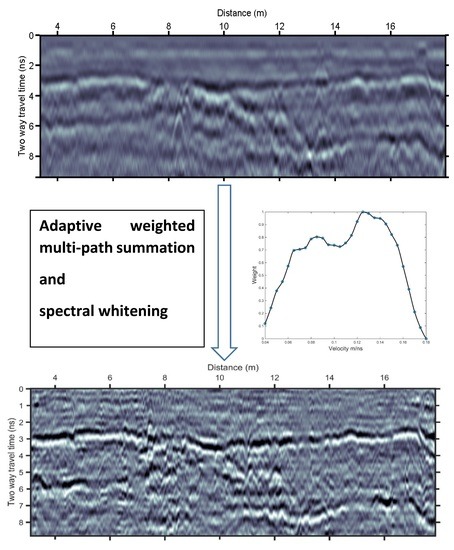
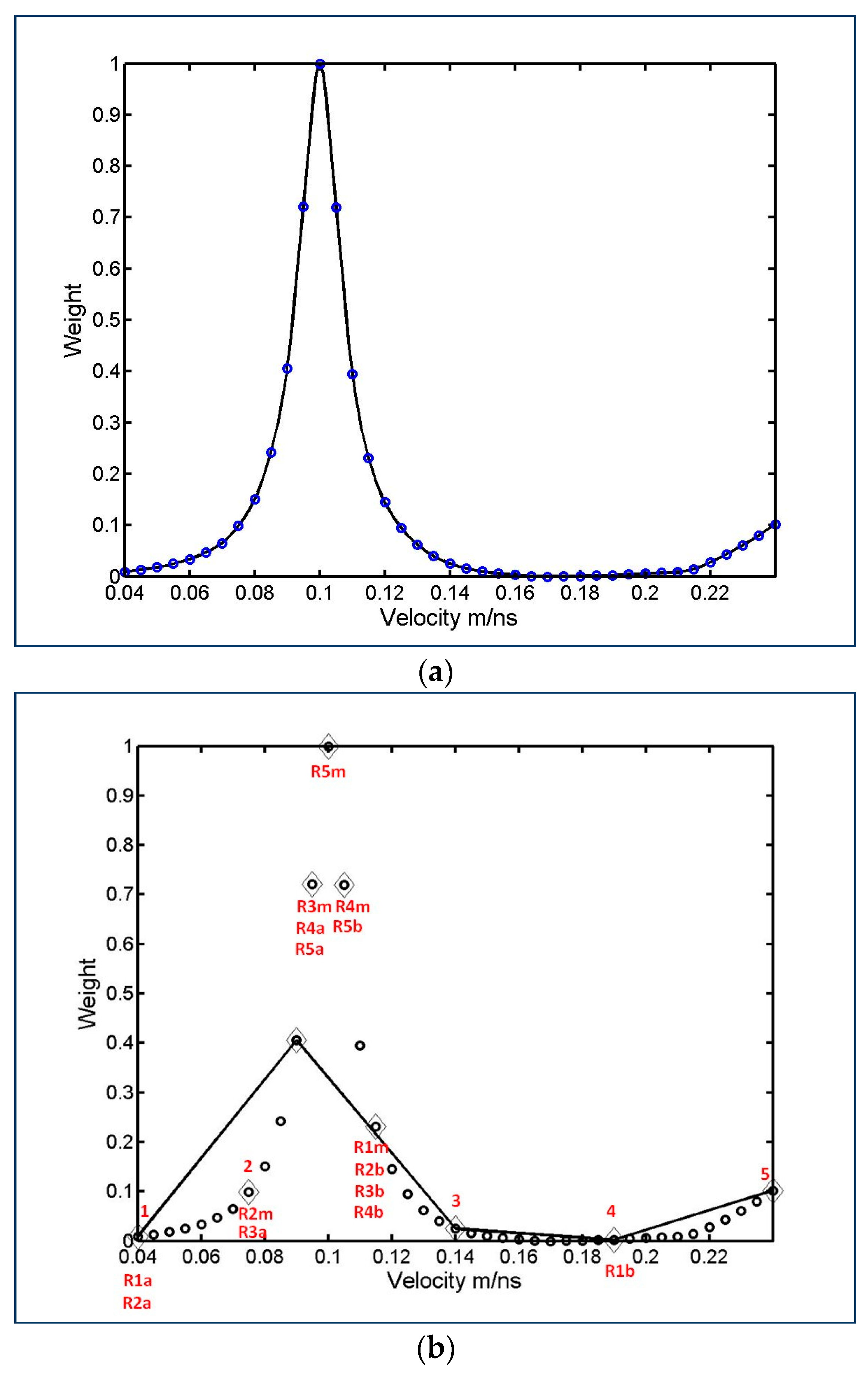
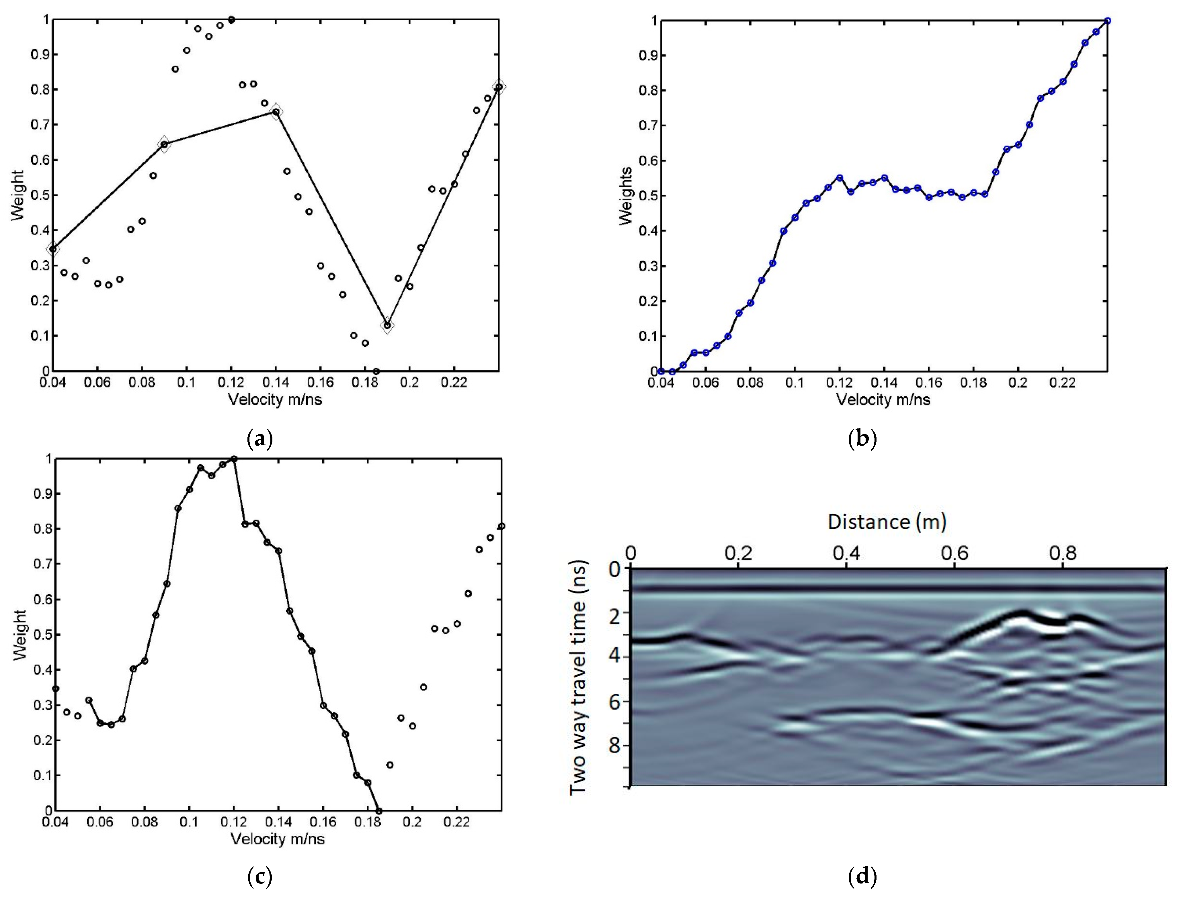
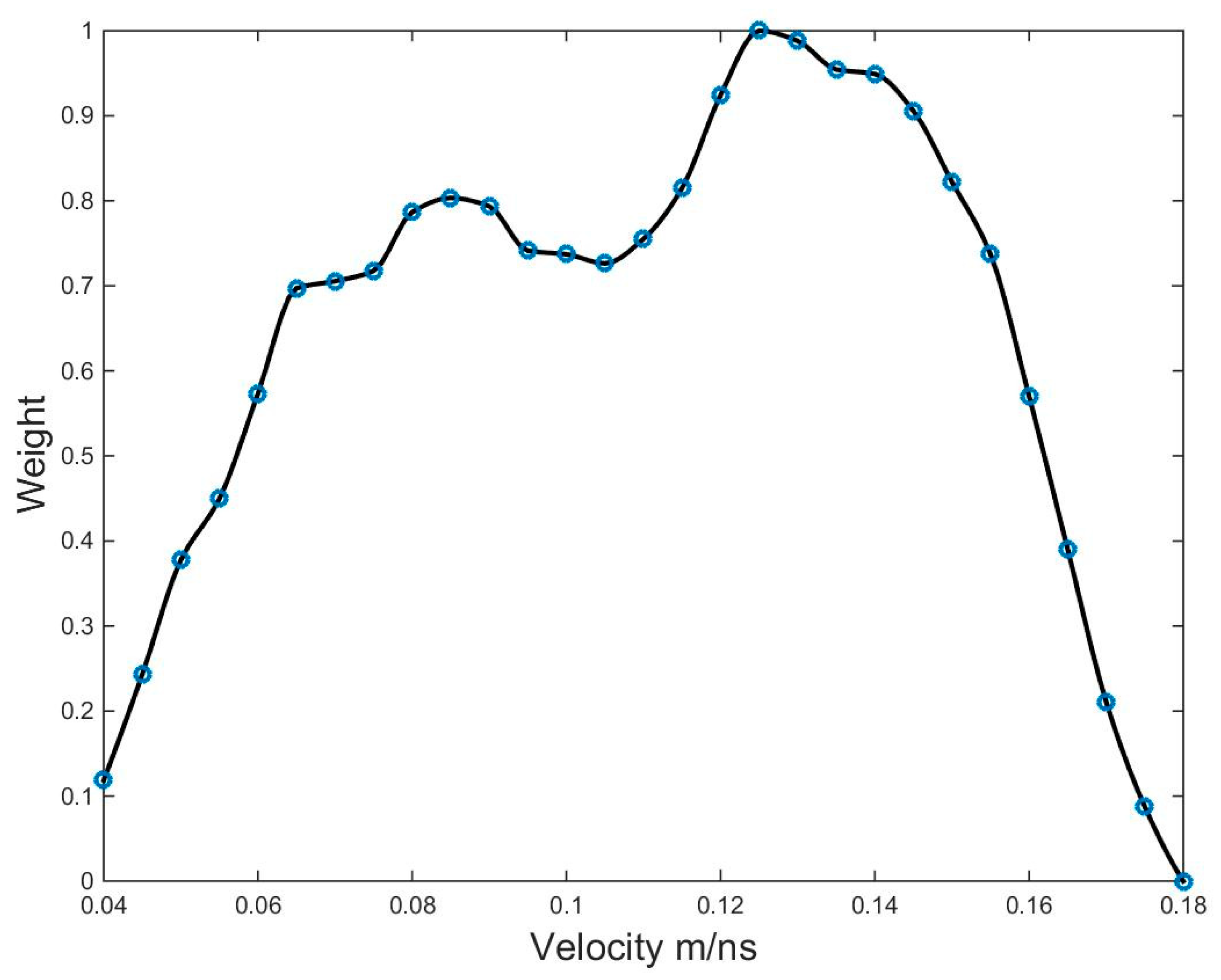
Adaptive choice of the velocities range and the stacking weights used for the multipath summation. We achieved this by employing a “divide and conquer” algorithm, which does not require any user action. In addition, it significantly reduces the computational cost by avoiding unnecessary migration velocity tests (with zero weight in the stacking process).
(2)
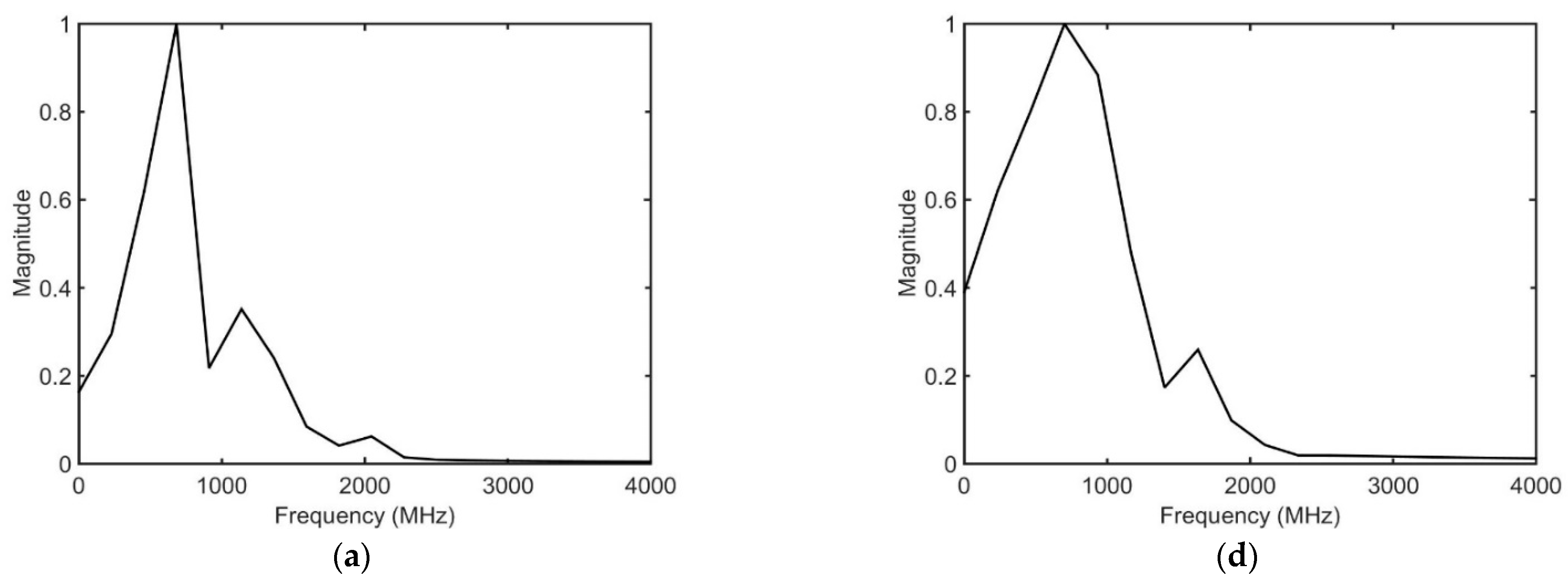
Adaptive spectral scaling for the time-varying spectral whitening, which is applied on the output of the multipath summation process. The amplitude spectral scaling used here whitens the amplitude spectrum within the passband of the traces. This is based on the use of time-gated spectra of the signal in the t-f domain, without the need for applying band pass filtering.

2. Methodology

The proposed methodology is based on the weighted multipath summation approach presented by Economou et al. [20]. To achieve our objective of reducing both the computational cost and the user interference, we employed the following processing steps:
  • Apply constant time-migration velocity scan of the GPR data using five specific velocity values covering the initial velocity range;
  • Apply a divide and conquer approach [25] to find the velocity values, which have optimum contribution to the final summation of the migrated sections;
  • Reapply constant time-migration velocity of the GPR data by using the velocity values not utilized in the previous steps [26];
  • Stack the weighted migration sections [20];
  • Apply adaptive spectrum scaling for time-varying spectral shaping of the multipath summation GPR section.

2.1. Evaluation of Constant Time-Migration Velocity Scan

As known, the success of migration relies on utilizing an appropriate velocity model. In order to explain our first step and to emphasize the importance of constant time-migration velocity scan, we exploited the same synthetic example adopted by Economou et al. [20]. This was based on the frequency–wavenumber modeling approach of Bitri and Grandjean [27]. It is a 1 m horizontal by 1 m depth model (Figure 1a–f) that consists of a homogeneous medium with 0.1 m/ns EM velocity as background. The time and space intervals of the synthetic data were set to 0.11 ns and 0.011 m, respectively. We inserted a point diffractor in the middle of the model, and we used a dominant frequency of 1 GHz for a Ricker wavelet. We also added random noise, normally distributed with zero mean and standard deviation (STD) equal to 10% of a mean trace STD (Figure 1a). We utilized Stolt’s f–k migration using five specific constant velocity values, ranging from 0.04 to 0.24 m/ns (Figure 1b–f). We can easily see the effect of under-migration (lower velocity value—Figure 1b,c) or over-migration (higher velocity value—Figure 1e,f). Using the correct velocity value (0.1 m/ns), however, efficiently focuses the energy of the diffraction to its apex. Nonetheless, the location of the apex of the hyperbola remains constant for all velocities used, since we utilize time migration.
We can evaluate the performance of each of the five constant velocity migrations used above by calculating their local slopes σ [20]. This can be accomplished using the local plane-wave equation:
P x + σ P t = 0 ,
where P is the wavefield and x and t are the space and time variables. Then, we utilized Claerbout’s [28] approach in order to estimate the partial derivatives in x and t directions:
C = [ a b a b a + b a + b ] A ,
where A is the data array, C is the matrix containing the partial derivatives, and * denotes 2D convolution. This operation is a convolution operation on the data matrix input and a 2 × 2 matrix kernel. When a = 1 and b = 0 or when a = 0 and b = 1, the partial derivatives in the x and t directions are calculated, respectively. In order to smooth the local slopes estimated from Equation (2), we applied a triangle-smoothing scheme [17,28,29]. This can be achieved by applying a 1D box smoothing twice. Repetition of this procedure makes the filter’s response approach a Gaussian shape, if desired. We can describe the triangle smoother mathematically using the following Z-transform notation, which is the result of correlating two box filters [15]:
T k ( Z ) = B k ( 1 / Z ) B k ( Z ) ,
with Bk(Z) being a box filter and k the filter length, we set the filter length for t direction to one-third of the dominant wavelet duration in all of our examples here, following Economou et al.’s [20] approach. One can also smooth the local slopes by Gaussian filtering or by using other types of band pass filters [17]. To apply triangle smoothing on a 2D array, one may apply triangle smoothing on both dimensions one by one. For the specific example of Figure 1, we achieved this by utilizing triangle operator lengths of 1.1 ns for t direction and 0.1 m for x direction, which corresponds to 10 samples for each direction. This gives us one-third of the dominant wavelet duration (3.3 ns in our case). If Cx and Ct are the arrays containing the partial derivatives in x and t directions, estimated by Equation (2), then we can calculate the local slopes using the following equation:
σ = C x t C t t , C t t 0 ,
where ∅ denotes dot or Hadamard division [30]. This is an element-by-element operation on two matrices of the same dimensions. C′xt and C′tt are the triangle-smoothed arrays where Cxt and Ctt are calculated using the equations:
C x t = C x   °   C t ,
C t t = C t   °   C t ,
where o denotes dot or Hadamardproduct [31].
To maintain numerical stability in our calculations, we need to avoid values close to zero for the denominator in Equation (4). Therefore, we do not account for values of σ when the absolute value of the denominator is smaller than 10−6. The parameter σ is estimated in (ns Δt)/(m Δx). Following Economou et al. [20], on all plotted images of local slopes in the present work, the angle σd is used
σd = arctan(σ),
which refers to the GPR image pixels (Figure 1d–f).
Once the local slopes are calculated (Figure 2a–f), we estimate the distribution of their global STD values. Figure 3 shows the resulting STD distribution of the local slopes estimated in Figure 2, which then can be used to evaluate the efficiency of velocity values used in the constant velocity migration. Lower STD values sections depict efficiently migrated sections (Figure 3d) while higher STD values are related to more unfocused diffractions (Figure 3a–c,e,f) within GPR sections. Hence, we can use the reciprocal values of calculated STDs to weight the contribution of the different velocities in stacking the migrated images (weighted path summation approach). The weights for each velocity can be normalized to their minimum and maximum values, as shown in Figure 4.
In the path-summation approach, we apply migration using a global velocity range that covers all commonly possible migration velocities within the GPR data set used. Usually a range of velocities between 0.04 and 0.24 m/ns with a step of 0.005 m/ns is employed. As expected, the smaller the velocity step used, the more efficient this approach will be in suppressing the hyperbolas tails to their apices. However, this will be on account of the computational cost, as the migration of each constant velocity section is time consuming. In order to reduce the time needed for this step, we propose using only five constant velocities initially, distributed over the above range. Therefore, we start with applying the constant velocity migration using the following starting constant velocities: 0.04, 0.09, 0.14, 0.19 and 0.24 m/ns.

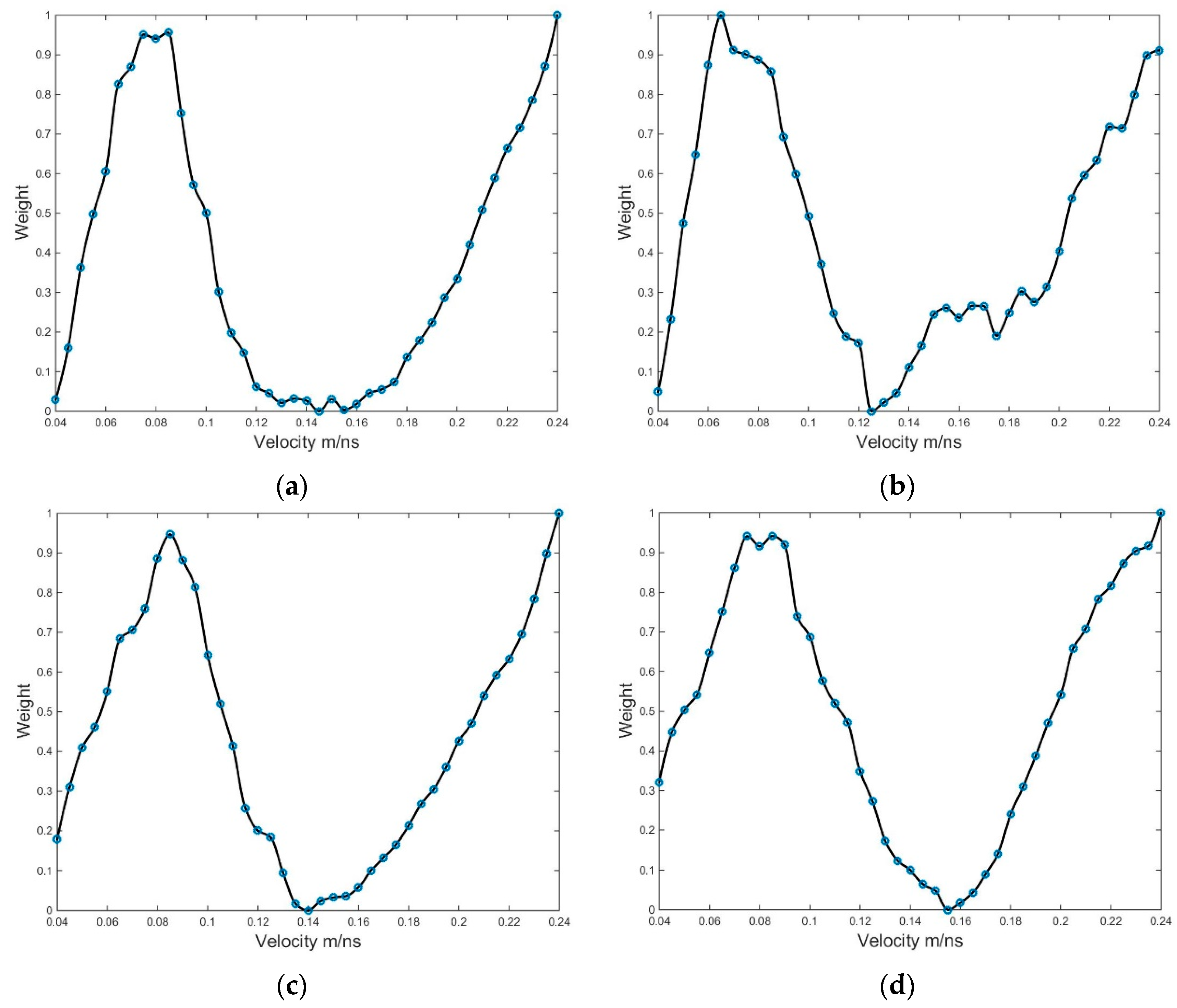
2.2. Divide and Conquer Approach

The second processing step utilizes the “divide and conquer” approach. Here, we exploit the relationship between the five initial chosen velocities and their assigned weights using the methodology explained above (diamonds denoted with red numbers 1, 2, 3, 4, and 5 in Figure 4b). We set our initial range of velocities (in which the maximum weight should occur) between the two minima (minimum assigned weights) among the chosen velocities. In our example in Figure 4b, the range is between 0.04 and 0.19 m/ns (diamonds symbolized as R1a and R1b). We then find the mean velocity value of these two, in our case this is 0.115 m/ns (denoted as R1m). We now need to further reduce the range of velocities, using these three new points (R1a, R1m, R1b) by finding the two with the largest weights. In our example, the new velocity range is between 0.04 and 0.115 m/ns (R2a and R2b). We then divide our new velocity range again by finding the midpoint between R2a and R2b, which is 0.075 m/ns (denoted as R2m in Figure 4b). We repeat the above procedure by conquering a new velocity range, based on the two maximum weights. Consequently, R2m (at 0.075 m/ns) becomes R3a and R2b (at 0.115 m/ns) becomes R3b. This “divide and conquer” approach is repeated until the new conquered range has a gap less than or equal to our velocity step (0.005 m/ns), which defines our final range of velocities in which the maximum weight exists. Here, the last points defining this narrow velocity range are the points indicated as R5a and R5b, which correspond to velocity values of 0.095 and 0.105 m/ns, respectively. The maximum weight is assigned to the middle point R5m for velocity value of 0.1 m/ns. Finally, this point’s position on the velocity axis indicates the final velocity values range, which is used for multipath summation. We achieve this by setting the lower velocity value as the initial minimum weight (0.04 m/ns in our case) and estimating its symmetrical to the right, namely 0.16 m/ns if 0.1 m/ns is set as the center. In our example, the final range of velocities has been significantly decreased compared to the initial global range of constant velocities used in the path-summation approach, reducing the computational cost of our proposed methodology. This procedure allows the user to find the constant velocities with the maximum migration weights, without the need to involve all velocities from the initial global range and without the need for user interference.

2.3. Completing the Constant Time-Migration Velocity Scan

Once we have defined the range of constant velocities with the optimum migration weights from the previous step, we need to perform the constant velocity migration on all the velocities within this range (0.04–0.16 m/ns with 0.005 m/ns step in our example). Considering that we have already calculated the migration sections for some points (diamonds in Figure 4b) in the previous divide and conquer step, here we complete the remaining velocity points (denoted as black circles in Figure 4b) within our velocity range. By adopting this approach, we have applied migration on 27 velocity points in total, including the 25 points within our defined velocity range, [(0.16 − 0.04)/0.005 + 1], plus the two values initially calculated outside the range (points 4 and 5). This results in significant saving of computational time compared to the 41 migrations [(0.24 − 0.04)/0.005) + 1] needed in the conventional path summation approach.

2.4. Stacking of Weighted Migration Sections

Now that we have performed the migration on all the constant velocity values within our range, we need to stack the weighted migration sections in order to focus the diffractions and enhance the lateral continuity. Let Ax,t be a GPR section and Ax,t,u the migrated GPR section using a constant velocity value u. The edges of our velocity range start from u1 to uN, where N is the number of the velocity values used. If Gu is a weighting function, then a weighted multipath summation section Bw,x,t can be estimated by
B w , x , t = 1 i = 1 N G u i i = 1 N [ A x , t , u i G u i ] ,

2.5. Applying Varying Spectral Shaping

The expected outcome of the previous stacking of the weighted migrated sections is a GPR section with focused diffractions. Howbeit, the wide range of velocities used usually ends in contaminating our final image, giving it a “blurry” texture. To overcome this issue we propose an adaptive time-varying spectral shaping technique, which is a modification of the Economou and Vafidis [32,33] and Economou et al. [20] approach. In this technique, we attempt to shape the initial amplitude spectrum of the traces to an amplitude spectrum with 1.5 times the peak frequency of the former. We achieve this by using time-gated spectra of the signal in the t-f domain. To reduce the user interference in this step, we propose a data adaptive scheme for the estimation of the reference amplitude spectrum used in the spectral shaping. We accomplish this by employing 12th-degree polynomials fitting through the Fourier transform (FT) of each time window. The inverse S-transform, which transforms the signal S(τ,f) in the t-f domain to the signal u(t) in time domain, is given by Stockwell et al. [34]:
u ( t ) = { S ( τ , f ) d τ } e i 2 π f t d f ,
where t is time, τ is time delay, and f is the frequency. The term in brackets is the FT of the signal. The split analytic signal in n/2 time-windows in the t-f domain can be retrieved by:
u a ( t ) = 0 f N { t 1 t 2 S ( τ , f ) d τ + t 3 t 4 S ( τ , f ) d τ t n 1 t n S ( τ , f ) d τ } e i 2 π f t d f ,
where fN is the Nyquist frequency, t1 = 0, and tn is the total recorded time of the signal, while integral term within the brackets corresponds to the FT of the specific duration, or the specific portion, of the signal. By replacing the FT with H(f) we obtain:
u a ( t ) = 0 f N { H 1 ( f ) + H 2 ( f ) + H k ( f ) } e i 2 π f t d f ,
where Hk is the spectrum of a specific duration of the time series. Note that we work only to the positive frequencies. If the same integral, with limits [−fN,0] and containing the conjugates of H1 to Hk, is combined with Equation (11), we have the inverse FT of the signal. Now, to apply spectral shaping for a portion of the time series, we use the following equation [31]:
| H b ( f ) | = { | H ( f ) | F ( f ) + max [ | H ( f ) | ] } F r ( f ) max [ F r ( f ) ] ,
where |H(f)| and |Hb(f)| are the input and output amplitude spectra of a time series (or its portion). Fr(f) is best-fit high-order polynomials for the reference amplitude spectrum. F(f) is the amplitude spectrum of the target signal. Equation (12) further requires that the energy of |Hb(f)| must be modified to be equal to the energy of |H(f)| [30]. To develop a more data adaptive scheme, we estimate the reference spectrum using the spectrum under processing by the Fourier transform (FT) scaling law:
u ( a t ) 1 a | H ( f a ) | e i φ ( f α ) ,
where u(t) is a time series, or portion of it, t is time, and f is frequency. The term H(f) = |H(f)|e(f) is the time series spectrum while α is the scaling factor. If we use α > 1, then the spectrum is shifted to a higher frequency band, increasing the time resolution. If we use 0 < α < 1, then we have the opposite effects. We modify only the amplitude spectrum, indicating a zero-phase procedure:
| H s ( f ) | = { 1 a 1 | H ( f a 1 ) | ,     0 f f p 1 a 2 | H ( f a 2 ) | ,                           f f p       ,
where |H(f)| is the amplitude spectrum of a portion of a time series in the t-f domain, |Hs(f)| is the scaled amplitude spectrum, α1 = 1 and α2 = 1.5, while fp is the peak frequency. In our case, Hs(f) is the reference spectrum for the implementation of Equation (12). The unity of the scaling factor α1, denotes that we simply keep the amplitude spectrum from zero frequency up to the peak frequency. On the other hand, we use the initial amplitude spectrum scaled 1.5 times its dominant frequency, for the peak frequency up to the Nyquist frequency. The latter also shifts the initial peak frequency value toward higher frequency values. This leaves a gap in between the lower frequencies amplitude spectrum and the higher frequencies amplitude spectrum. We use linear interpolation to fill this gap, which results in a white amplitude spectrum in between these two peak frequencies, and a naturally degrading spectrum at its edges. Afterward, we combine the amplitude spectrum |Hb(f)| with the initial phase spectrum to generate the zero-phased whitened spectrum of a portion of the time series. We then sum it with all of the time-portions-scaled spectra of the trace results in the scaled spectrum of the trace, according to the inverse S-transform relation (Equations (10) and (11)).

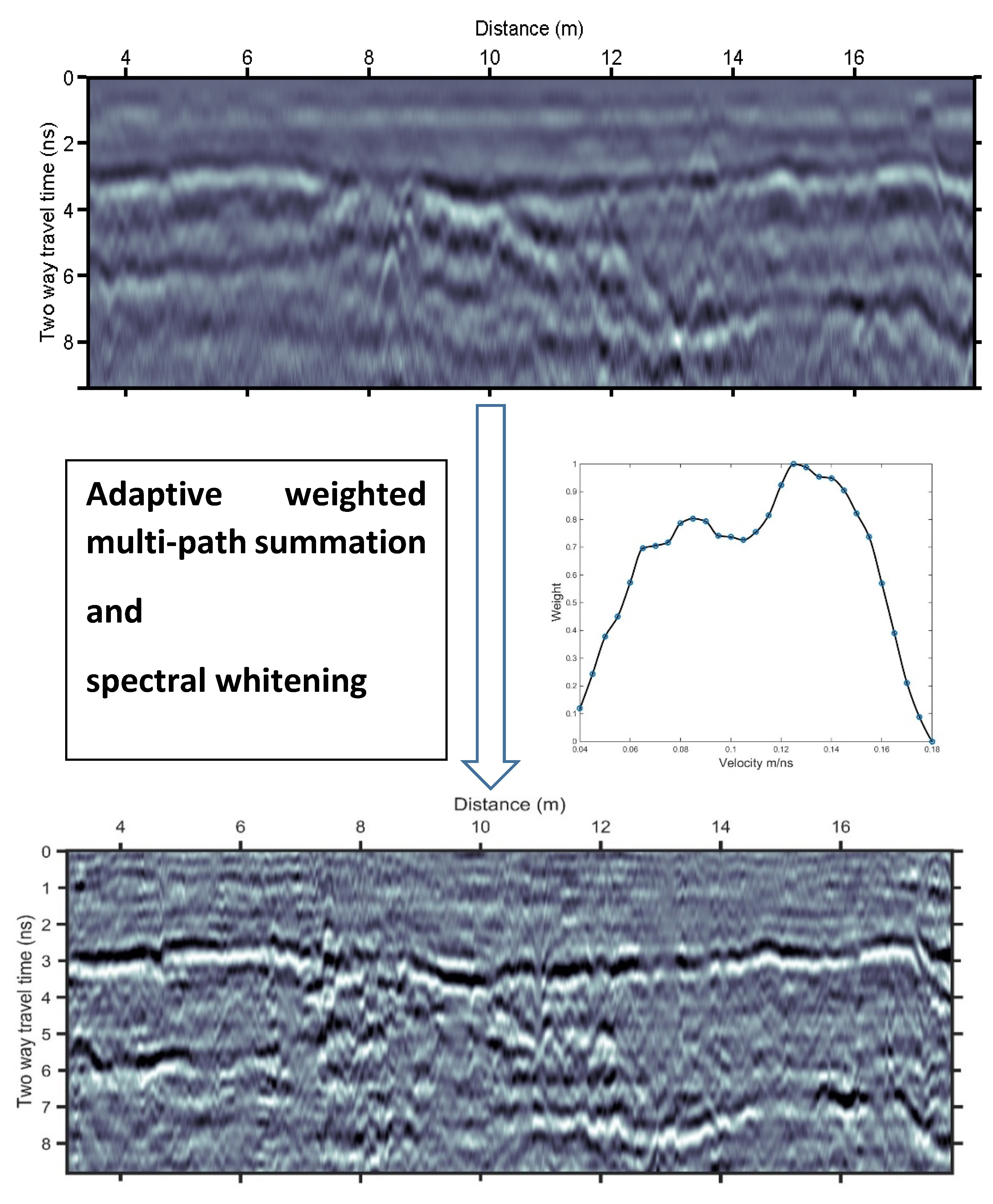
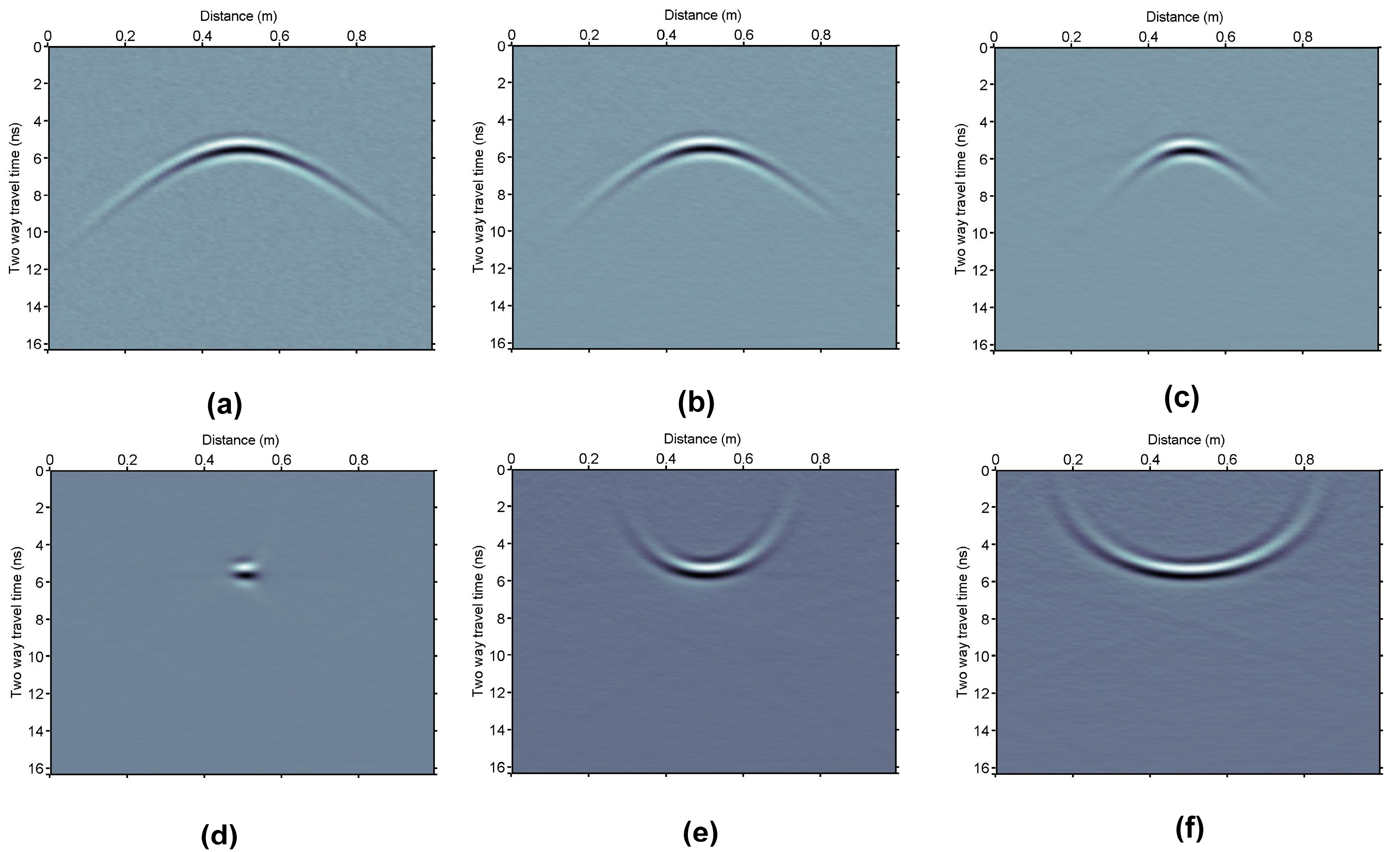
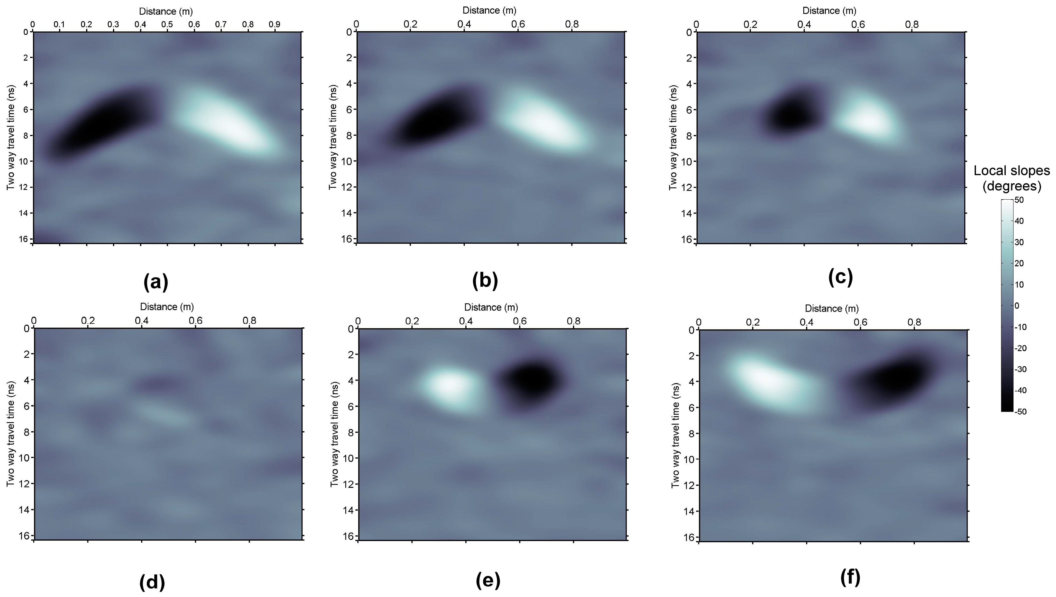
3. Synthetic Example
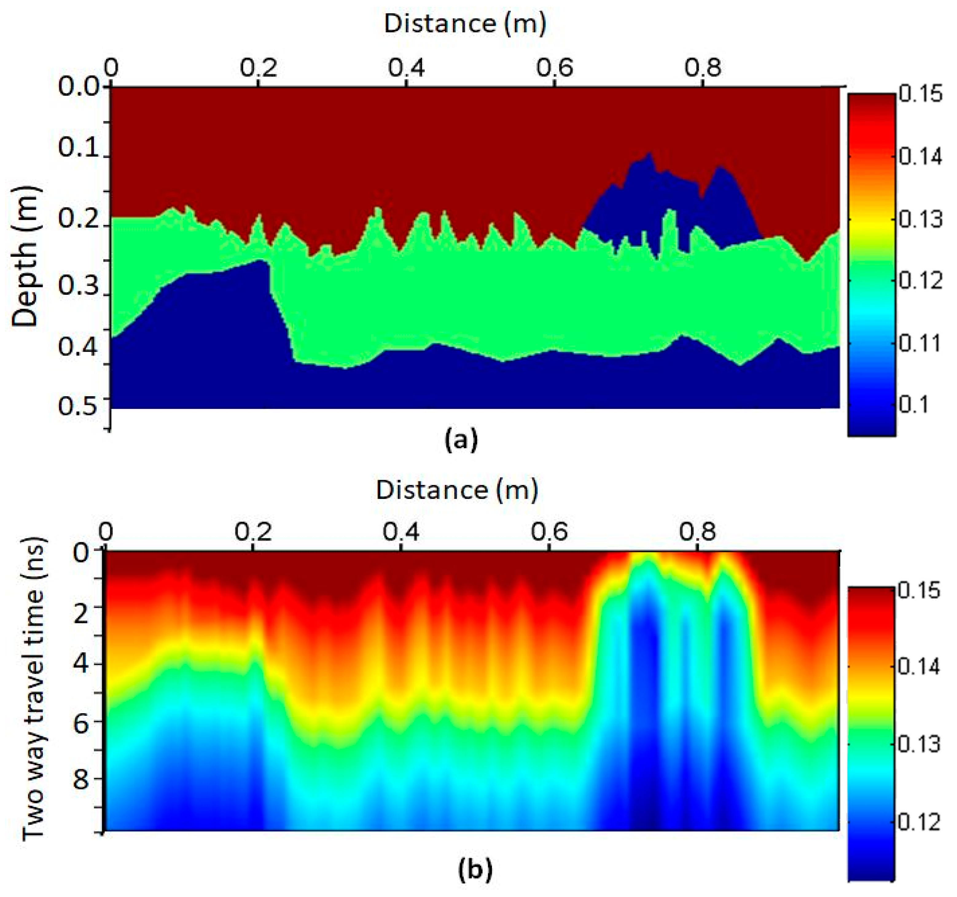
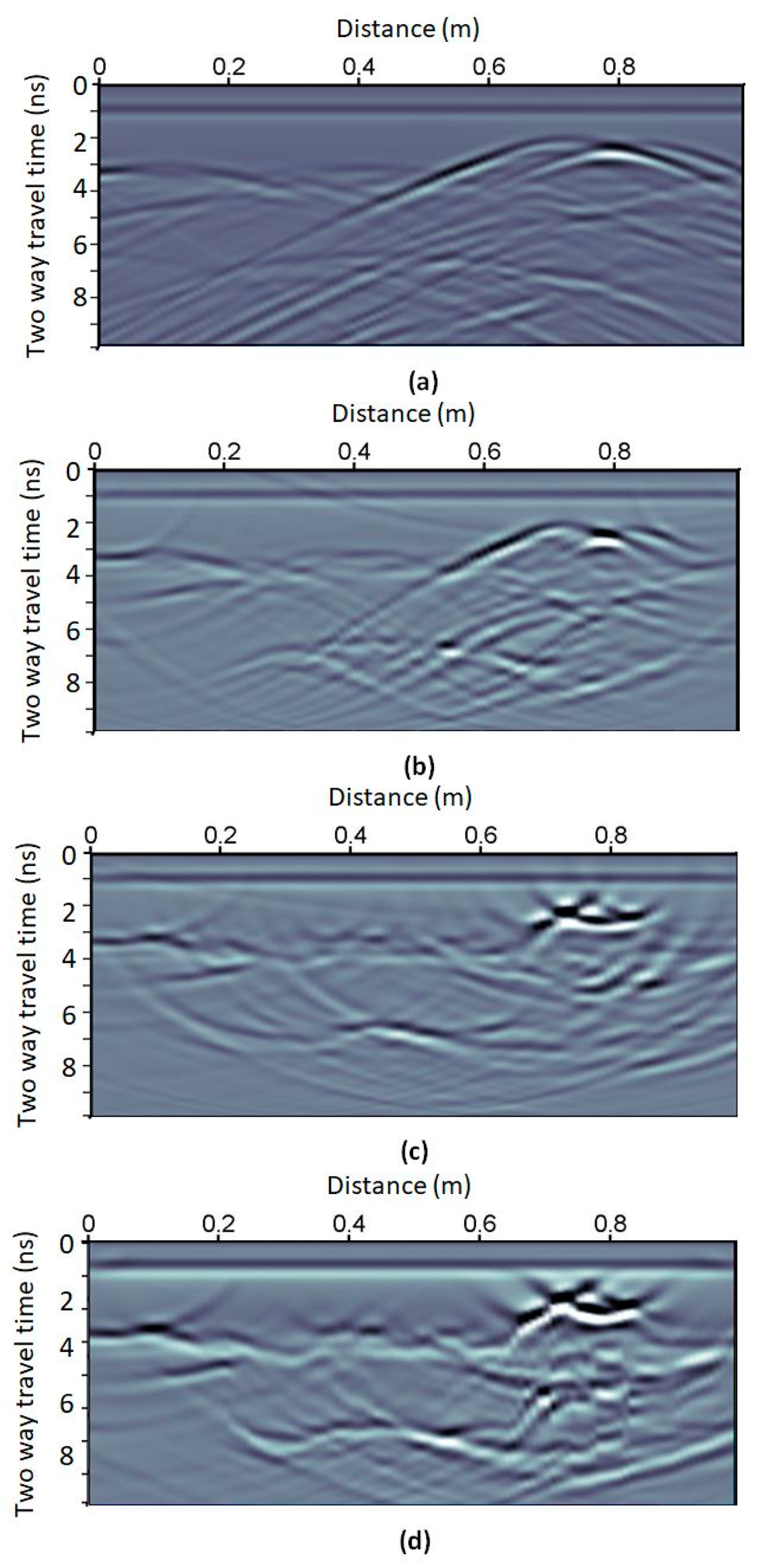
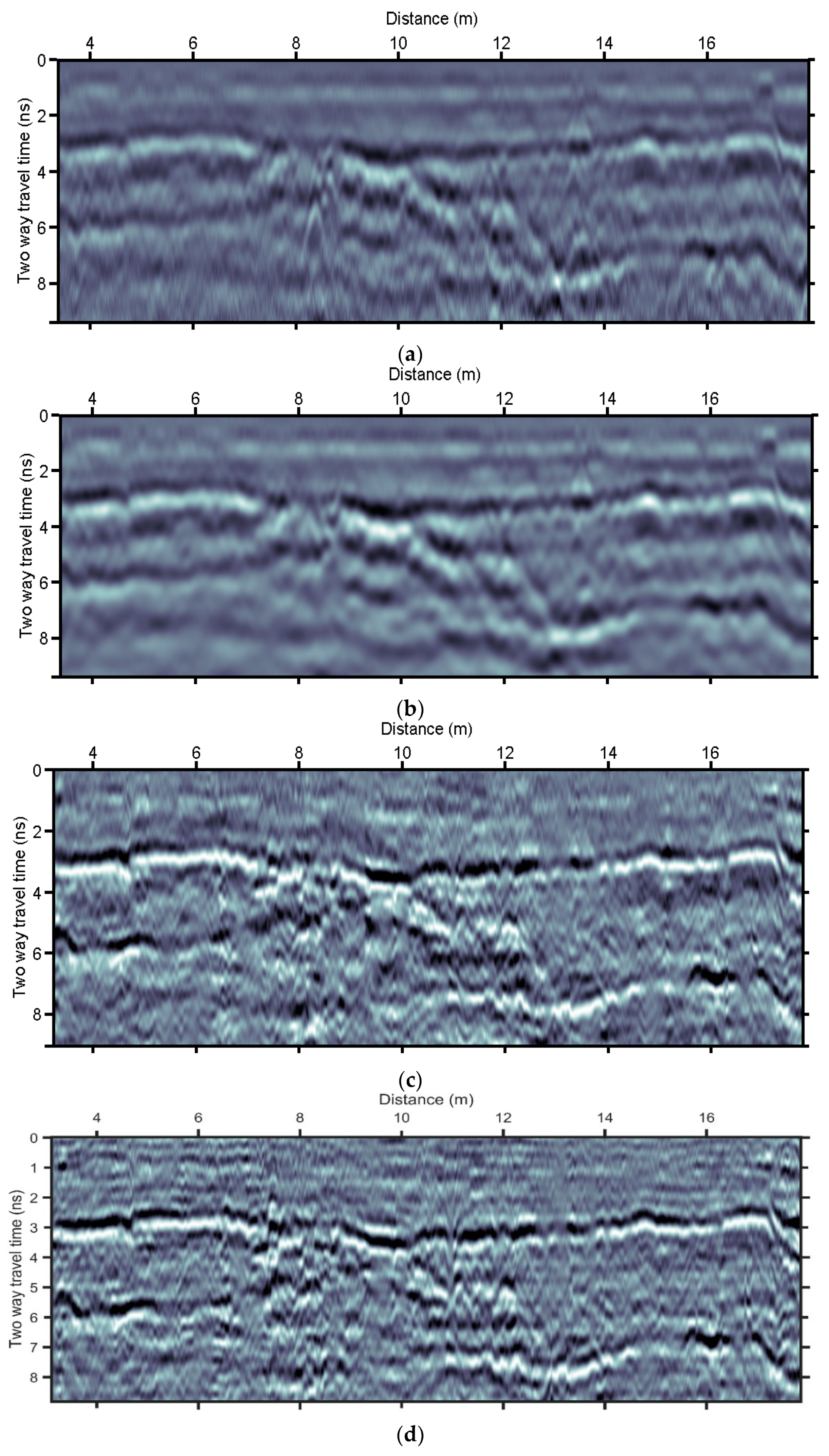
To evaluate our proposed approach, we used the Reflexw software version 9.1.3 [35] to generate a 1 m wide and 0.5 m depth data set. We employed Ricker wavelet with 1200 MHz dominant frequency, and a finite difference grid of 0.005 ns × 0.0005 m for time and scan directions, respectively. For the migration process, we obtained traces every 0.01 m and degraded the time interval to 0.05 ns, to simulate similar intervals used in true data acquisition. The electromagnetic (EM) velocities we used varied vertically and laterally from 0.1 to 0.15 m/ns, as shown in Figure 5a. The resulting synthetic GPR section (Figure 6a) lacks reflectors, as they are masked by diffractions. We tried to improve the lateral resolution by applying a constant velocity F-K migration using 0.12 m/ns velocity (Figure 6b), and one with constant velocity of 0.15 m/ns (Figure 6c). As expected, the former is more efficient at larger depths while the latter is focusing the diffracted energy at relatively early times because of the migration velocity used. Afterward, we applied Kirchhoff migration using the RMS velocities derived from the actual model (Figure 5b), which focused efficiently most of the GPR section (Figure 6d). Kirchhoff migration using the detailed known velocity model efficiently revealed the lateral nature of the reflectors and their correct locations (Figure 6d), much better than the constant velocity migrated sections (Figure 6b,c), but this is usually difficult to apply in real data since the actual velocity model is rarely known.
To apply the weighted multipath summation approach, we needed to estimate the local slopes required for stacking weights. We utilized triangle operator of 1 ns length for t direction and 0.2 m length for x direction, which corresponds to 20 samples for each direction. This gives us one-third of the dominant wavelet duration (3 ns in our data) as explained in Equation (3). Figure 7a shows the estimated weights, based on the local slopes, for a global range of velocities (0.04 m/ns to 0.24 m/ns) with 0.005 m/ns step, as per the approach proposed by Economou et al. [18].
We observed that a linear detrend of the weights is needed in most cases to smooth our data (Figure 7a). For our modified weighted multipath approach, we chose five distinct velocities among the global range: 0.04, 0.09, 0.14, 0.19, and 0.24 m/ns, to initialize the divide and conquer approach (Figure 7b, diamonds). Figure 7b depicts the weights after linear detrending the five velocities, shown with diamonds, but also the weight of all velocity values of Figure 7a for comparison (circles). By applying the proposed divide and conquer approach, we estimated the optimum velocity range (Figure 7c). We then applied the weighted migration on all velocities within the optimum velocity range and stacked them, resulting in the section presented in Figure 7d. It is clear that our proposed approach focused most of the diffracted energy and produced comparable results with that of the Kirchhoff migration, in terms of their lateral resolution. The resulting section shows accurately the location and continuity of the two reflectors with the possible exception of the first 20 cm of the second reflector, probably due to its steep slope. Still, our resulting section gives much better results than the conventional f–k migration results (Figure 6b,c) and similar information as shown in Figure 6d. The resolution of our section was degraded, however, because of the blurriness caused by stacking the migrated sections.

4. Real Data

We applied our proposed approach of data adaptive weighted multipath summation on two case studies of real GPR data sets. We chose one data set that is characterized by reflections and one data set with much diffraction, to better evaluate the efficiency of our approach on real complex data. For both case studies, we set a velocity range of 0.04 to 0.24 m/ns, in order to cover all the possible migration velocities, from saturated soils to dry sand. We kept the velocity interval to 0.005 m/ns as it proved efficient from the synthetic example.

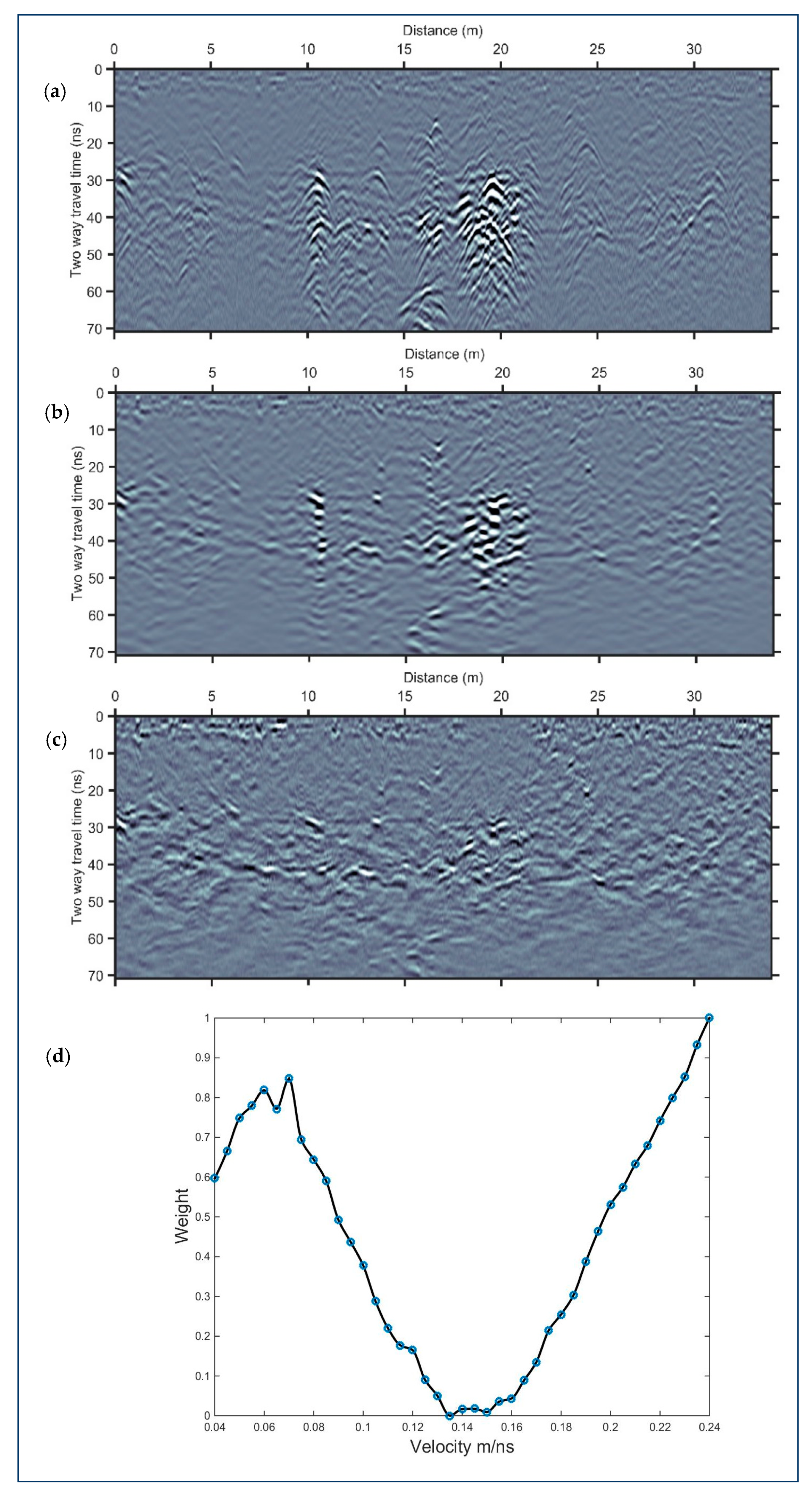
4.1. GPR Data Dominated by Reflections

The first data set comes from a utility detection survey, which also revealed the stratigraphy of the subsurface. The site is located in Abu Dhabi, UAE, where the main objective was to verify layout/routing of any existing underground utilities. The surface is flat and the subsurface formation consists mainly of silty sand. This data set was acquired using a GSSI 800 MHz antenna, where time and space intervals were set to 0.059 ns and 0.02 m, respectively. The initial processing included de-wow, band-pass filter, and time-varying gain (Figure 8a). Afterward, we estimated the local slopes employing a window operator of 20 × 20 size (time samples × number of traces), corresponding to 1.18 ns × 0.4 m, respectively. Based on the STD of the local slopes distribution, the weighted velocity range was set between 0.04 and 0.185 m/ns (Figure 9).
Weighted multipath summation focused most of the diffractions and adaptive spectral shaping technique managed to improve the resulting weighted multipath image resolution revealing the detailed subsurface stratigraphy (Figure 8b). The noise is suppressed and the diffractions are almost eliminated, even though the image resolution was degraded (blurriness) because of the migration velocities stacking. We manage to improve the image resolution significantly by applying the method of Economou and Vafidis [14] (Figure 8c). Still, this method needed the estimation of a reference amplitude spectrum, parameters regarding the effective frequency range for the application of the method, and a final band-pass to the output. The application of the proposed adaptive spectral shaping technique produced a similar output with increased resolution (Figure 8d). Both outcomes reveal the detailed subsurface stratigraphy, with good lateral resolution where most of the diffractions were eliminated.
To explain the effect of both methodologies, we plotted the amplitude spectra of two distinct events at 16 m from the origin of the data sections: the early arrival at 2.5 ns and the next strong event at 6.5 ns (Figure 8b). The amplitude spectra of these events are depicted in Figure 10a,d, respectively. An initial observation is the lower dominant frequency and spectrum width of the latter. The application of the method from Economou and Vafidis [14] adopts the scope of both increasing the resolution and restoring the dominant frequency stationarity, implemented as shown in Figure 10b,e, which are the corresponding amplitude spectra after spectral whitening. A reference wavelet was chosen from a shallower part of the section. Using the proposed methodology, spectral shaping the initial amplitude spectra, depicted in Figure 10a,d, increased the dominant frequency by also shifting the peak frequencies to almost 1.5 times the initial ones, but did not produce similar spectra, which would indicate dominant frequency stationarity. Still, the latter is fully adaptive and the output is similar to the conventional approach if one compares Figure 8c,d, which proves the similarity of the adaptive scheme output with the conventional scheme.

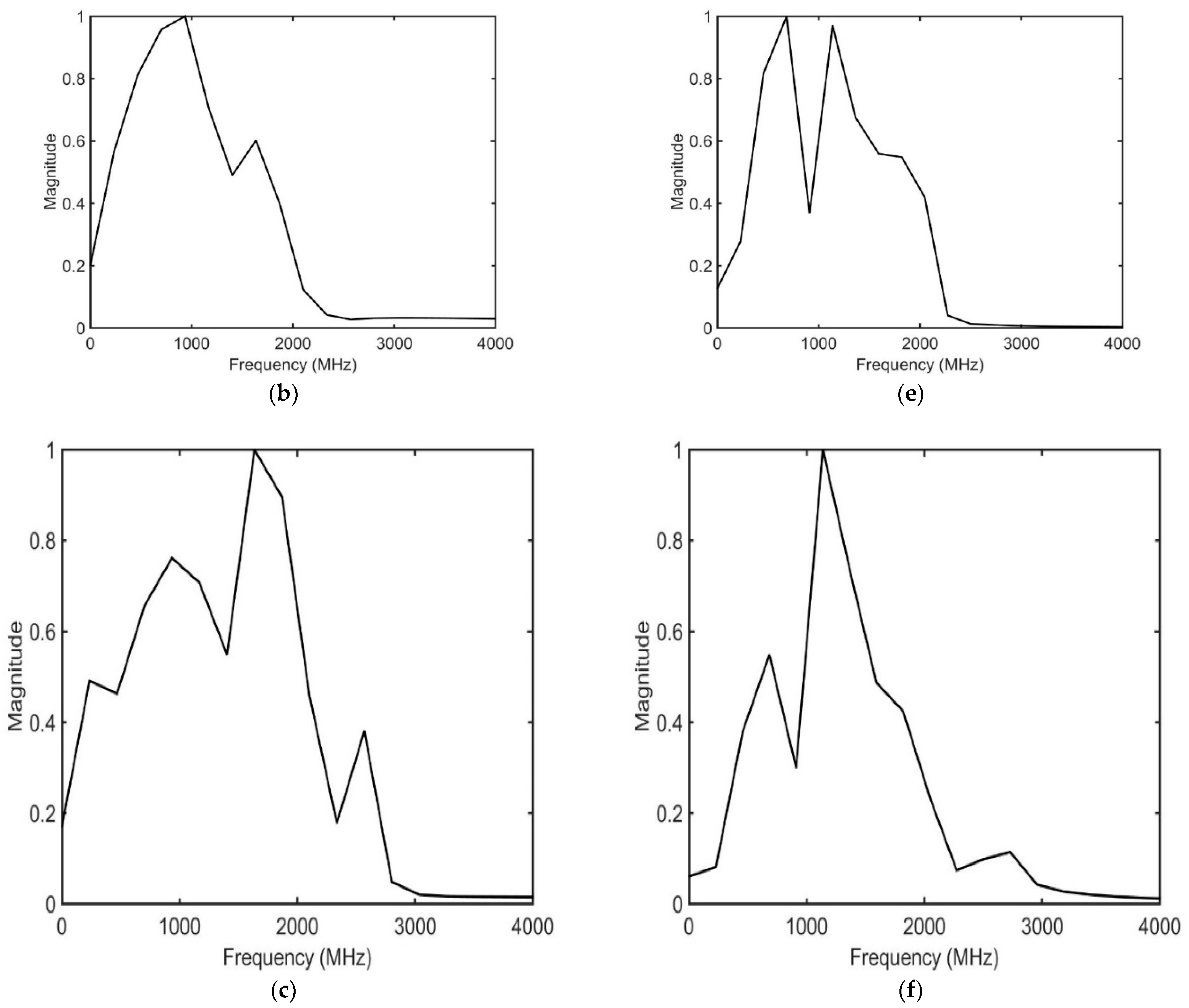
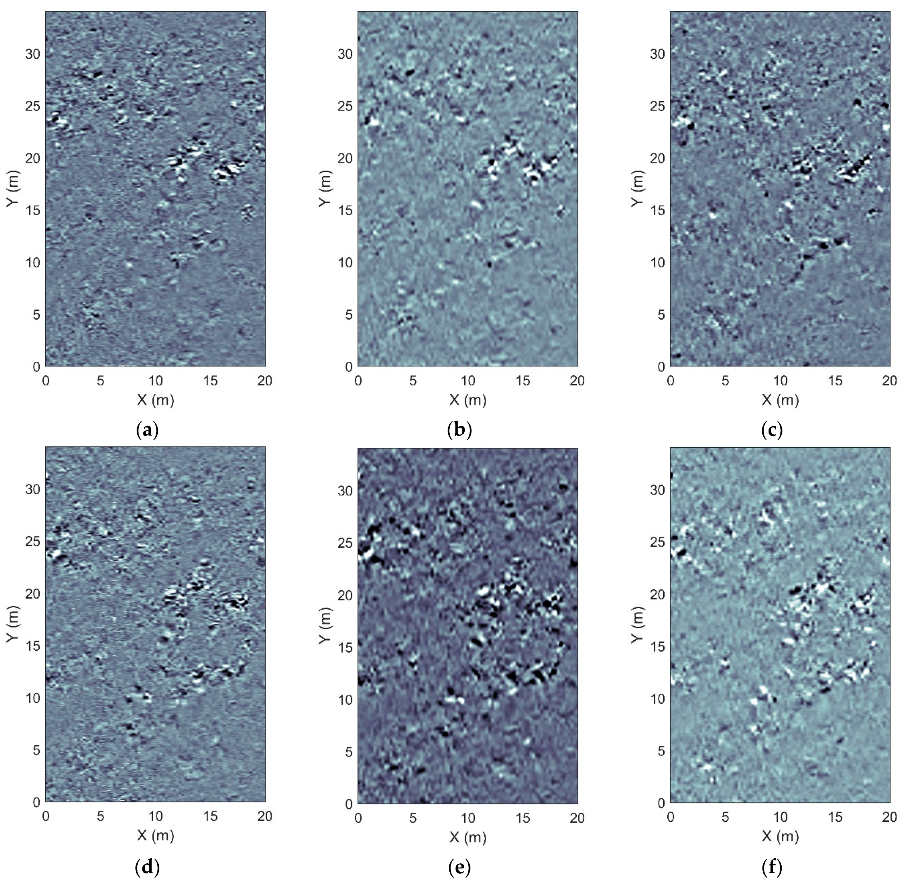
4.2. GPR Data Dominated by Diffractions

The second case study consists of a set of parallel GPR lines dominated by diffractions. The survey took place in the archeological site of Xochicalco in Mexico [36], where fractures and caverns are potential sources of the degradation of the archeological remains. The objective was to image weak zones in carbonates which may affect the stability of the walls remaining in Quetzalcoatl Temple. The subsurface consists mainly of pelagic limestones and breccias of the Xochicalco Formation [37] (Ruiz-Violante and Basañez-Loyola, 1994), where dissolution and cavern formation is expected. This case study helps us evaluate the applicability and efficiency of our proposed methodology on large data sets. The GPR survey was performed using a SIR-3000 system (GSSI) equipped with a shielded 400 MHz antenna. The GPR measurements were conducted in front of Quetzalcoatl Temple on a surface of 34 m × 20 m, involving 81 parallel study lines with lateral spacing of 0.25 m. The time interval was set to 0.1957 ns and the space interval to 0.02 m. Initial processing included time-zero shift, de-wow, and background removal filter of 200 traces, together with band-pass filtering 200–600 MHz and inverse exponential amplitude gain. A sample of the processed lines is presented in Figure 11a.
The data section after weighted multipath summation and spectral whitening is depicted in Figure 11b,c, respectively. The time-varying spectral whitening procedure reveals the detail of the lateral continuity of reflectors around 30 ns and 50 ns (Figure 11c). The windowing operator size for the local slopes estimation was set to (time samples × number of traces) = 20 × 20 corresponding to 3.9 ns × 0.4 m. The velocity range used for constant velocity migration and the evaluation of the STD of the local slopes distribution indicated a weighting function focusing to almost 0.075 m/ns (Figure 11d). The slope-dependent weighting function in Figure 11d underwent the proposed methodology for the adaptive estimation of the weights to be used for stacking and the weights within the range 0.04 to 0.15 m/ns was chosen. In Figure 11d and Figure 12, we show the whole range of velocities for the reader to see all the weights that would be estimated if the methodology of Economou et al. [20] was utilized. Economou et al. [36] utilized the methodology of Economou et al. [20] to extract depth slices from the specific data set. Namely, they estimated summation weights for the whole velocity range 0.04 to 0.24 m/ns and visually inspected the most appropriate weights to be further used for stacking constant velocity migration sections (Figure 11d and Figure 12).
Here, we applied the proposed methodology and adaptively estimated the same ranges of velocity values, without the need of user interference. These are representative results, while for all the other lines, the adaptive choice of weights was applied. This gave estimated ranges of 0.04–0.145, 0.04–0.125, 0.04–0.14, and 0.04–0.155 m/ns for Figure 12a–d, respectively. Note, except for the varying velocity ranges, the different peak values and the different shapes of the weighting functions. Similar variability but different values of velocity ranges and weights were chosen for each line of the whole 81 line data set, which demonstrates the need of the weights choice adaptiveness for such cases.
Horizontal time slices of the mean envelope of 31–36 ns (Figure 13a) and 37–42 ns (Figure 13d) were extracted, corresponding to approximately 1.65 and 1.87 m depths, respectively, for a mean velocity of 0.095 m/ns. The same time slices after multipath summation, except the focused energy, also indicate the increased blurriness (Figure 13b,e), which is avoided by the proposed spectral whitening method (Figure 13c,f).

5. Discussion

The weighted multipath summation method has been utilized by several researchers [18,19,20] to improve the lateral resolution of GPR sections by focusing the diffracted energy. The key word for the efficiency of the multipath summation is stacking. By stacking the different migrated sections using different velocities, the apices of the hyperbolas are enhanced against the moving tails of the over- or under-migrated parts of the constant velocity migrated sections. Therefore, after stacking the different migration sections, using the same range of constant velocity migration, this approach focuses most of diffracted energy despite spatial velocity variation. However, multipath summation images may suffer incomplete cancellation of the hyperbola tails due to not equally focused diffractions [19]. This is because the output of this methodology corresponds to an optimum combination of the existing migration velocities within the data, which produces an average focusing of all diffractions [19,20]. This is clear in Figure 8 and Figure 11 where some of the diffractions are not efficiently focused. Therefore, the main advantage of this approach is that it manages to focus most of the diffracted energy without requiring the knowledge or selection of a velocity model. Here, we presented a fully adaptive version of our previous approach of the weighted multipath summation method [20], with the scope to have a similar output, but with reduced computational and human intervention time.
We applied our proposed data adaptive approach on synthetic data dominated by diffractions, which masked the continuity of horizontal reflectors. Our approach managed to focus most of the diffracted energy and produced comparable results with that of the Kirchhoff migration, in terms of their lateral resolution, but without the need to build a velocity model. This was achieved with a significantly reduced number of constant velocity migrations compared to that of Economou et al.’s [20] approach and without the need of user intervention for finding the optimum weights. It is worth mentioning that the outcome of our proposed approach (Figure 7d) is closer to the real model than the ones of constant velocity migration (Figure 6b,c), but not as close as the outcome of the full velocity model migration (Figure 6d). The latter images also over-migrate artifacts due to the diffraction summation procedure of the Kirchhoff algorithm. Still, this outcome images the model in large details. The multipath summation outcome can be considered as a smoothed version of the Kirchhoff migrated section, which, although avoiding the migration procedure artifacts, it also lacks imaging detail. Finally, it should be noted that the high-dipping deeper reflector at a distance from almost 0.2 m to around 0.3 m is not imaged by any migration output as it is probably not recorded by the receiver; the reflected energy is transmitted further than the receiver’s position.
Encouraging results were also achieved when applying our approach on two different real data sets. The first was dominated by reflections while the second was dominated by diffractions. Our approach successfully suppressed most of the diffracted energy, improving the lateral resolution and emphasizing the accurate location of any reflectors. The expected degradation of the image resolution due to the introduced blurriness was remediated by the data-adaptive spectral whitening approach, with limited user interference. It was demonstrated that the adaptive scheme produces similar results as those with the conventional one, which is one of the main challenges for adaptive signal processing methods. Our approach was especially effective in reducing the computational time when applied to parallel GPR sections, as in the second real case study.
The interval of the study lines did not permit 3D migration, as aliasing would have occurred due to the large distance in comparison to the expected wavelength. Future research will focus on the implementation of a fully 3D approach. More effort will also be given in the direction of using our proposed focusing criteria for local focusing, which may lead to a migration velocity model to be used either for migration or for interpretational reasons.

6. Conclusions

We presented a strategy for adaptive diffraction focusing on zero-offset GPR data without the need to explicitly build a migration velocity model. We propose an improvement in the multipath summation method in order to reduce the user intervention in its implementation, and provide an alternative implementation of the local slopes estimation stage. We employed a “divide and conquer technique” for estimating the range of velocities to be used in the constant velocity migration in order to reduce the migrations needed and, subsequently, the implementation time. The alternative approach for estimating the local slopes presented here does not involve abstract vectors as in Economou et al. [20], but rather the x and t partial derivatives in data matrices. We also introduced a modified spectral scaling scheme for the spectral whitening of the results in migrated GPR sections. This method effectively restores the blurriness introduced by constant velocity migrated sections stacking and the migrations themselves, without the need to estimate a reference wavelet or other parameters for whitening stability, as well as a final band-pass to the output. The final output of applying our proposed data adaptive methodology managed to improve the lateral continuity of GPR sections, similar to our previous methodology. The need for a detailed velocity model is suppressed, and the user’s involvement is restricted to specifying a range of trial velocity values instead of applying velocity analysis, which usually requires multioffset GPR data. This velocity range can be wide enough to include velocity values that characterize the formations of the area under investigation.

Author Contributions

Conceptualization, H.H. and N.E.; Data curation, H.H., N.E. and J.O.-R.; Methodology, H.H., N.E. and M.B.; Software, N.E.; Supervision, A.V. and M.B.; Validation, A.V.; Writing—original draft, H.H. and N.E.; Writing—review & editing, A.V., M.B. and J.O.-R. All authors have read and agreed to the published version of the manuscript.

Funding

This research received no external funding.

Data Availability Statement

The data presented in this study are available on request from the corresponding author. The data are not publicly available due to privacy restriction.

Conflicts of Interest

The authors declare no conflict of interest.

References

  1. Özdemir, C.; Demirci, F.; Yilit, E.; Yilmaz, B. A review on migration methods in B-Scan Ground penetrating radar imaging. Math. Probl. Eng. 2014, 2014, 280738. [Google Scholar] [CrossRef] [Green Version]
  2. Olhoeft, G.R. Electromagnetic field and material properties in ground penetrating radar. In Proceedings of the 2nd International Workshop on Advanced Ground Penetrating Radar, Delft, The Netherlands, 14–16 May 2003; pp. 144–147. [Google Scholar] [CrossRef]
  3. Liu, L.; Li, Z.; Arcone, S.; Fu, L.; Huang, Q. Radar wave scattering loss in a densely packed discrete random medium: Numerical modeling of a box-of-boulders experiment in the Mie regime. J. Appl. Geophys. 2013, 99, 68–75. [Google Scholar] [CrossRef]
  4. Wei, X.; Zhang, Y. Autofocusing Techniques for GPR Data from RC Bridge Decks. IEEE J. Sel. Top. Appl. Earth Obs. Remote Sens. 2014, 7, 4860–4868. [Google Scholar] [CrossRef]
  5. Feng, D.; Li, T.; Li, G.; Wang, X. Reverse time migration of GPR data based on accurate velocity estimation and artifacts removal using total variation de-noising. J. Appl. Geophys. 2022, 198, 104563. [Google Scholar] [CrossRef]
  6. Sun, J.; Young, R. Recognizing surface scattering in ground-penetrating radar data. Geophysics 1995, 60, 1283–1597. [Google Scholar] [CrossRef]
  7. Özdemir, C.; Demirci, S.; Yigit, E. Practical Algorithms to Focus b-Scan GPR Images: Theory and Application to Real Data. Prog. Electromagn. Res. B 2008, 6, 109–122. [Google Scholar] [CrossRef] [Green Version]
  8. Bradford, J.H. Measuring water content heterogeneity using multi-fold GPR with reflection tomography. Vadose Zone J. 2008, 7, 184–193. [Google Scholar] [CrossRef]
  9. Bradford, J.H. Reverse-time prestack depth migration of GPR data from topography for amplitude reconstruction in complex environments. J. Earth Sci. 2015, 26, 791–798. [Google Scholar] [CrossRef]
  10. Forte, E.; Pipan, M. Review of multi-offset GPR applications: Data acquisition, processing and analysis. Signal Process. 2017, 132, 210–220. [Google Scholar] [CrossRef]
  11. Greaves, R.; Lesmes, D.; Lee, J.; Toksöz, M. Velocity variations and water content estimated from multi-offset ground-penetrating radar. Geophysics 1996, 61, 627–993. [Google Scholar] [CrossRef]
  12. Smitha, N.; UllasBharadwaj, D.R.; Abilash, S.; Sridhara, S.; Singh, V. Kirchhoff and F-K migration to focus ground penetrating radar images. Int. J. Geo-Eng. 2016, 7, 4. [Google Scholar] [CrossRef] [Green Version]
  13. Dou, Q.; Wei, L.; Magee, D.R.; Cohn, A.G. Real-Time Hyperbola Recognition and Fitting in GPR Data. IEEE Trans. Geosci. Remote Sens. 2017, 55, 51–62. [Google Scholar] [CrossRef] [Green Version]
  14. Yuan, H.; Montazeri, M.; Looms, M.; Nielsen, L. Diffraction imaging of ground-penetrating radar data. Geophysics 2019, 84, H1–H12. [Google Scholar] [CrossRef]
  15. Novais, A.; Costa, J.; Schleicher, J. GPR velocity determination by image-wave remigration. J. Appl. Geophys. 2008, 65, 65–72. [Google Scholar] [CrossRef]
  16. Clair, S.J.; Holbrook, W.S. Measuring snow water equivalent from common-offset GPR records through migration velocity analysis. Cryosphere 2017, 11, 2997–3009. [Google Scholar] [CrossRef] [Green Version]
  17. Fomel, S. Shaping regularization in geophysical estimation problems. Geophysics 2007, 72, R29–R36. [Google Scholar] [CrossRef]
  18. Landa, E.; Fomel, S.; Moser, T.J. Path-integral seismic imaging. Geophys. Prospect. 2006, 54, 491–503. [Google Scholar] [CrossRef]
  19. Merzlikin, D.; Fomel, S. Analytical path-summation imaging of seismic diffractions. Geophysics 2017, 82, S51–S59. [Google Scholar] [CrossRef]
  20. Economou, N.; Vafidis, A.; Bano, M.; Hamdan, H.; Ortega-Ramirez, J. Ground-penetrating radar data diffraction focusing without a velocity model. Geophysics 2020, 85, H13–H24. [Google Scholar] [CrossRef]
  21. Burnett, W.; Fomel, S.; Bansal, R. Diffraction velocity analysis bypath-integral seismic imaging. In Proceedings of the 81st Annual International Meeting, SEG, Expanded Abstracts, San Antonio, TX, USA, 18–22 September 2011; pp. 3898–3902. [Google Scholar]
  22. Schleicher, J.; Costa, J.C. Migration velocity analysis by double path-integral migration. Geophysics 2009, 74, WCA225–WCA231. [Google Scholar] [CrossRef] [Green Version]
  23. Santos, H.; Schleicher, J.; Novais, A.; Kurzmann, A.; Bohlen, T. Robust time-domain migration velocity analysis methods for initial-model building in a full waveform tomography workflow. In Proceedings of the 78th Annual International Conference and Exhibition, EAGE, Extended abstract, Vienne, Austria, 15–20 September 2019. [Google Scholar] [CrossRef]
  24. Economou, N.; Vafidis, A. GPR data time varying deconvolution by kurtosis maximization. J. Appl. Geophys. 2012, 81, 117–121. [Google Scholar] [CrossRef]
  25. Xia, G.; Sin, M.; Stoffa, P. 1-D Elastic Wave Inversion: A divide-and-conquer approach. Geophysics 1998, 63, 1670–1684. [Google Scholar] [CrossRef] [Green Version]
  26. Hamdan, H.; Economou, N.; Vafidis, A. Data Adaptive GPR Diffraction Focusing Using Multi-Path Summation. In Proceedings of the 26th European Meeting of Environmental and Engineering Geophysics, Online Conference, 7–8 December 2020; Volume 2020, pp. 1–5. [Google Scholar] [CrossRef]
  27. Bitri, A.; Grandjean, G. Frequency—Wavenumber modelling and migration of 2D GPR data in moderately heterogeneous dispersive media. Geophys. Prospect. 1998, 46, 287–301. [Google Scholar] [CrossRef]
  28. Claerbout, J.F. Earth Soundings Analysis: Processing versus Inversion, 1st ed.; Blackwell Scientific Publications: Hoboken, NJ, USA, 2004. [Google Scholar]
  29. Hale, D. Local dip filtering with directional laplacians. GWP Proj. Rev. 2007, 567, 91–102. [Google Scholar]
  30. Cyganek, B. Object Detection and Recognition in Digital Images: Theory and Practice, 1st ed.; John Wiley & Sons: Hoboken, NJ, USA, 2013; p. 109. ISBN 9781118618363. [Google Scholar]
  31. Million, E. The Hadamard Product. 2007. Available online: http://buzzard.ups.edu/courses/2007spring/projects/million-paper.pdf (accessed on 1 October 2021).
  32. Economou, N.; Vafidis, A. Spectral balancing of GPR data using time-variant bandwidth in t-f domain. Geophysics 2010, 75, J19–J27. [Google Scholar] [CrossRef]
  33. Economou, N.; Vafidis, A. Deterministic deconvolution for GPR data in t-f domain. Near Surf. Geophys. 2011, 9, 427–433. [Google Scholar] [CrossRef]
  34. Stockwell, R.G.; Mansinha, L.; Lowe, R.P. Localization of the complex spectrum: The S-transform. IEEE Trans. Signal Process. 1996, 44, 998–1001. [Google Scholar] [CrossRef]
  35. Sandmeier, K. Reflex Manual 2019; Version 9.0; Sandmeier Geophysical Research: Karlsruhe, Germany, 2019; Available online: www.sandmeier-geo.de (accessed on 1 April 2021).
  36. Economou, N.; Bano, M.; Ortega-Rameriz, J. Delineation of Fractures Using a 2D GPR Processing Strategy for 3D Imaging: Weak Zones within Carbonates at the Archaeological Site of Xochicalco in Mexico. Appl. Sci. 2021, 11, 5893. [Google Scholar] [CrossRef]
  37. Ruiz-Violante, A.; Basañez-Loyola, M. La Formacion Xochicalco, Unidad estratigráfica del Albiano-Cenomanianoenlos Estados de Morelos, Guerrero y México. In Proceedings of the XII Convención Geológica Nacional, Sociedad Geológica Mexicana, Toluca, Mexico, 1994; pp. 161–162. [Google Scholar]
Figure 1. Constant velocity migration of a simulated GPR section containing one diffractor into a homogeneous velocity background equal to 0.1 m/ns. (a) Simulated GPR data with additive white noise. Constant velocity migration of (a) by using a velocity value of (b) 0.04, (c) 0.07, (d) 0.1, (e) 0.16, and (f) 0.24 m/ns. Adapted with permission from Ref. [20].
Remotesensing 14 02547 g001
Figure 2. Estimated local slopes for the GPR sections shown in Figure 1: (a) local slope of simulated GPR data with additive white noise in Figure 1a; (bf) local slopes of the migrated sections of Figure 1b–f respectively. Adapted with permission from Ref. [20].
Remotesensing 14 02547 g002
Figure 3. The distribution of the global STD values of the estimated local slopes for (a) raw GPR data; migrated sections using constant velocity equal to (b) 0.04, (c) 0.07, (d) 0.1, (e) 0.16, and (f) 0.24 m/ns.
Remotesensing 14 02547 g003
Figure 4. Comparison between (a) the constant velocity points and their estimated weights used for stacking the migrated data in the path summation approach, and (b) the procedure of the “divide and conquer” approach for the optimum velocity range for multipath summation.
Remotesensing 14 02547 g004
Figure 5. Velocity model for the simulation of GPR data: (a) velocity model; (b) RMS velocity model based on (a).
Remotesensing 14 02547 g005
Figure 6. Simulation of GPR data: (a) simulated GPR data; (b) simulated GPR data after constant velocity migration with 0.12 m/ns velocity and (c) 0.15 m/ns; (d) shows (a) after migration using the velocity model depicted in Figure 5b.
Remotesensing 14 02547 g006
Figure 7. Construction of a data-dependent weighting function and multipath summation: (a) stacking weights using the reciprocal values of local slopes STD values from each of the constant velocity migrated data, employing velocities within the range 0.04 to 0.24 m/ns and step 0.005 m/ns; (b) shows (a) after detrend (circles) and the initial velocity values chosen for the divide and conquer approach (diamonds); (c) estimated optimum weights for constant velocity migrated sections stacking and (d) is the output of stacking.
Remotesensing 14 02547 g007
Figure 8. Real example dominated by reflections: (a) GPR data obtained using a 800 MHz GSSI shielded antenna over silty sand; (b) weighted multipath summation using the local slopes distribution as a weighting function (Figure 9); (c) shows (b) after spectral whitening using the method presented by Economou and Vafidis [31,32]; and (d) shows (b) after spectral whitening using the proposed methodology of time-varying spectral scaling.
Remotesensing 14 02547 g008
Figure 9. Constant velocity migrated data stacking weights as estimated by the proposed methodology, referring to the data depicted in Figure 8a.
Remotesensing 14 02547 g009
Figure 10. Representative amplitude spectra of selected events: (a) amplitude spectra of a distinct event at 16 m and 2.5 ns, shown in Figure 8b; (b) corresponding amplitude spectra of (a) after spectral whitening; (c) corresponding amplitude spectra of (a) after using our approach; (d) amplitude spectra of a distinct event at 16 m and 6.5 ns, shown in Figure 8b; (e) corresponding amplitude spectra of (d) after spectral whitening; (f) corresponding amplitude spectra of (a) after using our approach.
Remotesensing 14 02547 g010aRemotesensing 14 02547 g010b
Figure 11. Real example dominated by diffractions: (a) example of GPR data obtained using a 400 MHz GSSI shielded antenna over carbonates around the middle (10 m) of parallel GPR lines covering an area of 20 m; (b) weighted multipath summation using the local slopes distribution dependent weighting function in (d) and velocity values range 0.04 to 0.15 m/ns and step 0.005 m/ns; (c) shows (b) after spectral whitening and (d) is the whole velocity range stacking weights.
Remotesensing 14 02547 g011
Figure 12. Stacking weights estimated for representative GPR lines of a 3D acquisition (parallel study lines) over an area of 34 × 20 m. From (ad), corresponding GPR study lines located at 1, 6, 16 and 19 m.
Remotesensing 14 02547 g012
Figure 13. Horizontal depth slices of the 3D data acquisition example. The first row of images corresponds to the mean amplitude of 31 to 36 ns, or approximately at 1.65 m depth of (a) the initially processed data, (b) the multipath summation data, and (c) the spectral whitened data of (b). The second row of images (df) depicts the same information as above for the mean amplitude of 37 to 42 ns or approximately at depth 1.87 m.
Remotesensing 14 02547 g013
Publisher’s Note: MDPI stays neutral with regard to jurisdictional claims in published maps and institutional affiliations.

