An Optimal Transport Based Global Similarity Index for Remote Sensing Products Comparison

Abstract

Remote sensing products, such as land cover data products, are essential for a wide range of scientific studies and applications, and their quality evaluation and relative comparison have become a major issue that needs to be studied. Traditional methods, such as error matrices, are not effective in describing spatial distribution because they are based on a pixel-by-pixel comparison. In this paper, the relative quality comparison of two remote sensing products is turned into the difference measurement between the spatial distribution of pixels by proposing a max-sliced Wasserstein distance-based similarity index. According to optimal transport theory, the mathematical expression of the proposed similarity index is firstly clarified, and then its rationality is illustrated, and finally, experiments on three open land cover products (GLCFCS30, FROMGLC, CNLUCC) are conducted. Results show that based on this proposed similarity index-based relative quality comparison method, the spatial difference, including geometric shapes and spatial locations between two different remote sensing products in raster form, can be quantified. The method is particularly useful in cases where there exists misregistration between datasets, while pixel-based methods will lose their robustness.

1. Introduction

With the quick and great development of remote sensing technologies, together with the spread of open science, there are many available similar remote sensing products, and global land cover products are very typical examples, which are typically presented as digital thematic maps in raster. Thus, to facilitate common users’ easy-to-choose appropriate products, the need to compare their accuracy is growing. An ideal accuracy assessment is based on comparing a dataset with its true value; however, usually, it is impossible to obtain ‘ground truth’ in practice, thus accuracy assessments are usually conducted by comparing the dataset with some ‘reference data’. We know that remote sensing products from different sources are different in many aspects, including data source, classification scheme, methodology and resolution, etc. [1]. This is not surprising, given the fact that quantitative analyses of complex land cover types remain an arduous task [2].

2. Related Works

Table 1. Relative comparison methods.

Comparison Methods		Processing Unit	Qualitative/Quantitative	Evaluating Indicator	Attention Scale
Error Matrix-based methods	Pixel-by-pixel based Statistical method [3,4,5]	pixel	qualitative	OA, UA, PA, kappa coefficient, information entropy, etc.	Local scale
			quantitative	Mean, standard deviation, entropy, correlation coefficient, Tau coefficient, etc.
	Quantity and location-based method [6]		qualitative	Location-based kappa coefficient, quantity-based kappa coefficient, etc.
local spatial feature-based methods	Spatial distribution-based method [7,8,9]	category	qualitative	Goodman–Kruskal Cramér’s V statistics Theil’s U statistics	Global scale
	Neighborhood-based comparison method [10]			Spatial structure and overlap index
Other methods	Fuzzy comparison [11,12]	pixel and category	qualitative	Fuzzy Kappa coefficient fuzzy similarity index.	Specific scope
	Curvature-fit based method [13,14]	category		Polygon matching index	Specific scope
	Sliding-window based method [15]	sliding window	quantitative	Euclidean distance, correlation coefficient

lists some commonly used relative comparison methods of remote sensing products. Considering their definition, processing units and evaluating indicators, relative comparison methods can be classified into three categories: error matrix-based, local spatial feature-based and others. In these methods, spatial features are expressed at three scales: (i) a local scale for statistical analysis of pixels, (ii) a global scale for analysis of the whole image, and (iii) specific scopes, such as sliding windows.

Existing relative comparison methods are mostly based on the confusion or error matrix method [16,17]. However, error matrix-based methods ignore the underlying geometry of the space. For example, the blue pixels in Figure 1 represent water bodies. It is clear that the error matrix, user’s accuracy, and producer’s accuracy in datasets 2 and 3 are the same (because the number of water pixels is the same). However, it is obvious that the spatial positions of the two different areas in datasets 2 and 3 are different compared to dataset 1, and the difference between dataset 2 and dataset 1 is more like a real water body than an error. Therefore, the spatial distribution of “errors” and the information contained in the “errors” are also very important in a relative quality evaluation system. Moreover, the validation techniques based on pixel statistics rely heavily on probability sampling design for collecting validation data [3]. In the error matrix-based methods, reference data are taken as real data, and some studies have shown that if errors in the reference data are related to the predicted data, the comparison accuracy will be overestimated, and if the error is conditional independent, the accuracy will be underestimated [18]. The kappa coefficient based on the error matrix is also considered to be unsuitable [19].

Researchers have proposed some improved methods based on the error matrix. For example, Enøe et al. [20] used a maximum likelihood method to deal with unknown binary reference data. However, this method can only verify the reference data and cannot revise the result. The authors of [21] proposed to simulate the geometric deviation in different directions with a certain step size based on the reference image, and then calculate the geometric accuracy of coarse-resolution remote sensing data by calculating the correlation between the migrated reference image and the image to be evaluated, while there are still uncertainties in determining the size of step. To sum up, these methods based on error matrix lack the description of the spatial structure of remote sensing products.

In order to comprehensively consider and quantify the possible spatial features in different remote sensing products in the form of raster datasets, we attempted to design a “similarity index” by taking raster datasets as the probability distributions in a two-dimensional space, and then measured the difference between two distributions, thus the problem of accuracy comparison between different raster datasets is turned into a multi-category optimal transmission question. Therefore, in fact, it is now a question of spatial similarity measurement.

Optimal transport theory gives a good framework for comparing two measures in a Lagrangian framework, and Wasserstein distance is an important concept arising from optimal transport, which are the metrics of probability distributions. At present, some applications of optimal transport theory in the field of remote sensing have been proposed [22] to fuse remote sensing products with social media information by using the natural interpretation of distribution distance in Wasserstein metric space [23] using high-resolution satellite time-series images to evaluate the accuracy of remote sensing mapping products in the absence of field verification data by using EMD transmission and Sinkhorn transmission.

The optimal transport theory establishes a geometric tool for effectively comparing probability distributions. The relative similarity concept in the paper is based on max-sliced Wasserstein distance [24]. The main contributions of this paper are the following:

(i)

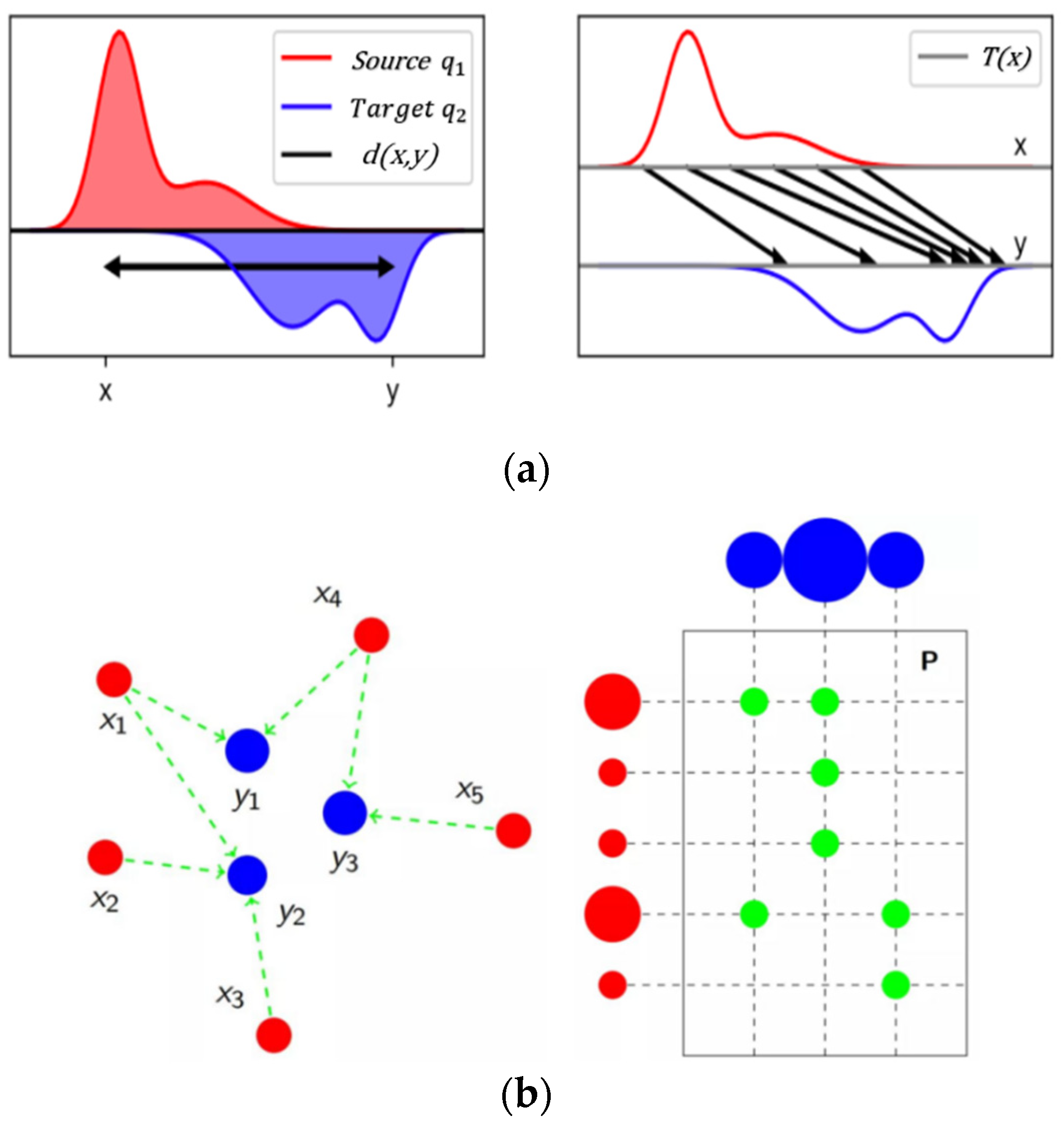
Category information contained in multi-source raster datasets is treated as a probability distribution of spatial information in a 2D space, and then the problem of consistency measurement between remote sensing products is converted into a measurement question of probability distribution.

(ii)

A max-sliced Wasserstein distance-based similarity index is designed and calculated, which could solve the product comparison problem in the case of misregistration.

3. Methodology

Wasserstein distance provides a way to measure the distance between two non-empty datasets, and a raster dataset can be taken as a set of multiple types of pixel coordinates, so this measurement applies.

Wasserstein-P distance between two pixel-based distributions $q_1$and $q_2$could be expressed as follows:

$$W_P\left(q_1,q_2\right)={\left(\underset{\gamma \left(x,y\right)\in \Gamma \left(q_1,q_2\right)}{inf}{E}_{\left(x,y\right)~\gamma \left(x,y\right)}[d\left(x,y{)}^P\right]\right)}^{\frac{1}{P}}$$

(1)

where x,y are the distribution of pixel coordinates in the two raster datasets, respectively,$\Gamma \left(q_1,q_2\right)$ is the set of all possible joint distributions on (x,y) with marginals $q_1$ and $q_2$, d(x,y) is the distance metric between $x$ and $y$, generally, the Euclidean distance is taken. In a two-dimensional case, P = 2.

Figure 2a illustrates the one-dimensional case, that is, using the minimum cost to convert one distribution into another distribution. Figure 2b is a two-dimensional case, using a transmission matrix P to describe the transmission plan.

In fact, it is difficult to calculate the Wasserstein distance in two or more dimensions directly through the optimal transport theory. Kantorovich–Rubinstein duality can be used to calculate its one-dimensional case:

$$W\left(q_1,q_2\right)=\underset{\Vert f{\Vert }_L\leqq 1}{sup}{E}_{x~q_1}\left[f\left(x\right)\right]-E_{x~q_2}\left[f\left(x\right)\right]$$

(2)

where the supremum is over all the 1-Lipschitz functions $f \mathrm{X}\to \mathrm{R}$. The function $f$ is commonly represented via a deep net and various ways have been suggested to enforce the Lipschitz constraint [25].

Then, a sliced version of the Wasserstein-2 distance, proposed by [26], shows its advantage, which only requires estimating distances of one-dimensional distributions and is more efficient. The “sliced Wasserstein-p distance” between distributions $q_1,q_2$ is defined as:

$${\tilde{W}}_{\mathrm{p}}\left(q_1,q_2\right)={[ \underset{\mathsf{\omega }\in \mathsf{\Omega }}{{\displaystyle \int }}{W}_P^P\left(q_1^{\omega },q_2^{\omega }\right)d\mathsf{\omega }]}^{\frac{1}{P}}$$

(3)

where $q_1^{\omega },q_2^{\omega }$ denote the projection (i.e., marginal) of $q_1,q_2$ onto the direction $\mathsf{\omega }$, and$\mathsf{\Omega }$ is the set of all possible directions on the unit sphere.

The ${\tilde{W}}_{\mathrm{p}}\left(q_1,q_2\right)$distance has important practical implications: provided that the projected distributions $q_1^{\omega },q_2^{\omega }$ can be computed, then for any $\mathsf{\omega }\in \mathsf{\Omega }$, the distance ${\tilde{W}}_{\mathrm{p}}\left(q_1,q_2\right)$, as well as its optimal transport map and the corresponding Kantorovich potential can be analytically computed by using projected measures that are one-dimensional.

For two given datasets $\mathit{D}=\left\{\left(\mathrm{x}\right)\right\}$of samples $\mathrm{x}\sim q_1$,$\mathit{F}=\left\{\left(\mathrm{y}\right)\right\}$of samples $\mathrm{y}\sim q_2$:

$$W_2^2\left({\mathit{D}}^{\omega },{\mathit{F}}^{\omega }\right)=\frac{1}{\left|\mathit{D}\right|}{\displaystyle \sum }_{i=1}^{\left|\mathit{D}\right|}\Vert {\mathit{D}}_{\phi \mathit{D}\left(i\right)}^{\omega }-{\mathit{F}}_{\phi \mathit{F}\left(i\right)}^{\omega }\Vert {}_2^2$$

(4)

where $\phi \mathit{D}$and $\phi \mathit{F}$ are permutations that sort the projected sample sets ${\mathit{D}}^{\omega }$ and ${\mathit{F}}^{\omega }$, respectively.

$${\mathit{D}}_{\phi \mathit{D}\left(1\right)}^{\omega }\le {\mathit{D}}_{\phi \mathit{D}\left(2\right)}^{\omega }\le \cdots \le {\mathit{D}}_{\phi \mathit{D}\left(\left|\mathit{D}\right|\right)}^{\omega }$$

(5)

$${\mathit{F}}_{\phi \mathit{F}\left(1\right)}^{\omega }\le {\mathit{F}}_{\phi \mathit{F}\left(2\right)}^{\omega }\le \cdots \le {\mathit{F}}_{\phi \mathit{F}\left(\left|\mathit{F}\right|\right)}^{\omega }$$

(6)

When the number of elements in the two datasets $\left|\mathit{D}\right|$,$\left|\mathit{F}\right|$ are different, find the greatest common divisor $\mathsf{\theta }$ of $\left|\mathit{D}\right|$ and $\left|\mathit{F}\right|$, then make ${\left|\mathit{D}\right|}^{*}=\frac{\left|\mathit{F}\right|}{\mathsf{\theta }}$, ${\left|\mathit{F}\right|}^{*}=\frac{\left|\mathit{D}\right|}{\mathsf{\theta }}$, and replace $\mathit{D}\left(i\right)$ with ${\left|\mathit{D}\right|}^{*}$ elements, together with replacing $\mathit{F}\left(i\right)$ with ${\left|\mathit{F}\right|}^{*}$ elements. Because ${\left|\mathit{D}\right|}^{*}\left|\mathit{D}\right|={\left|\mathit{F}\right|}^{*}\left|\mathit{F}\right|$, it is sure that the element numbers in the two new sets are the same.

If we could find the most meaningful projection direction, the 2D max-sliced-Wasserstein distance will be calculated, and it is defined as follows:

$$max-{\tilde{W}}_2\left(q_1,q_2\right)={\left[ma{x}_{\omega \in \Omega }{W}_2^2\left(q_1^{\omega },q_2^{\omega }\right)\right]}^{\frac{1}{2}}$$

(7)

This metric satisfies the properties of non-negativity, the identity of indiscernible, symmetry, and subadditivity [27]. Hence, it is a true metric.

Taking two land cover datasets, A and B, with K categories and the size of $\mathrm{Row}\times \mathrm{Col}$ as an example, after each$max-{\tilde{W}}_2$ is calculated by categories, the similarity between A and B can be defined:

$$\begin{gathered} Similarity\left(A,B\right)= \\ {\displaystyle \sum }_{\mathrm{i}=1}^{\mathrm{K}}[1-\frac{1}{\sqrt[2]{{\mathrm{Row}}^2+{\mathrm{Col}}^2}}\times min(\sqrt[2]{{\mathrm{Row}}^2+{\mathrm{Col}}^2},\frac{max-\widetilde{W_2}\left(i\right)}{1-\frac{N\left(i\right)}{\mathrm{Row}\times \mathrm{Col}}})]\times \frac{N\left(i\right)}{\mathrm{Row}\times \mathrm{Col}} \end{gathered}$$

(8)

where $max-\widetilde{W_2}\left(i\right)$ is the max-sliced Wasserstein distance of category$i$, and N(i) is the average number of pixels of category i in datasets A and B, that is, $N\left(i\right)=\frac{1}{2}\left[N_A\left(i\right)+N_B\left(i\right)\right]$.

It could also be deduced that the similarity between two datasets is order independent, so we have:

$$Similarity\left(A,B\right)=Similarity\left(B,A\right)$$

(9)

This method has the following advantages: (1) It can quantify the difference in both spatial position and shape, then measure it under a unified standard; (2) it can give a continuous transformation process while preserving geometric features; (3) it has symmetry and can still give reasonable measurement results in the case of regional misregistration.

4. Experiment

To demonstrate the rationality of the above-proposed similarity index, we designed several validation experiments both on test datasets and real datasets. For test datasets, we set four cases, and use a gradient descent method to give the continuous transformation process. For real datasets, we calculate the similarity index among three open land cover products.

4.1. Experiments on Test Datasets

(i)

Max-sliced Wasserstein distance between two points

Suppose there are two points on the two-dimensional plane, the coordinates of the two points are (9.0, 9.0) and (13.0, 12.0), respectively.

The results of the max-sliced Wasserstein distance with the number of projections and the percentage difference with the Euclidean distance are shown in

Table 2. Distance with the number of projections.

Number of projections	5	10	15	20
Max-Wasserstein distance	4.9700	4.9961	4.9970	4.9994
Difference	0.6%	0.078%	0.06%	0.012%

.

The Euclidean distance between the two points is 5.0. Because the sliced distance is calculated by using projection, there is a deviation from the Euclidean distance. We consider that when the number of projections is not less than 20, the deviation is within the allowable range.

(ii)

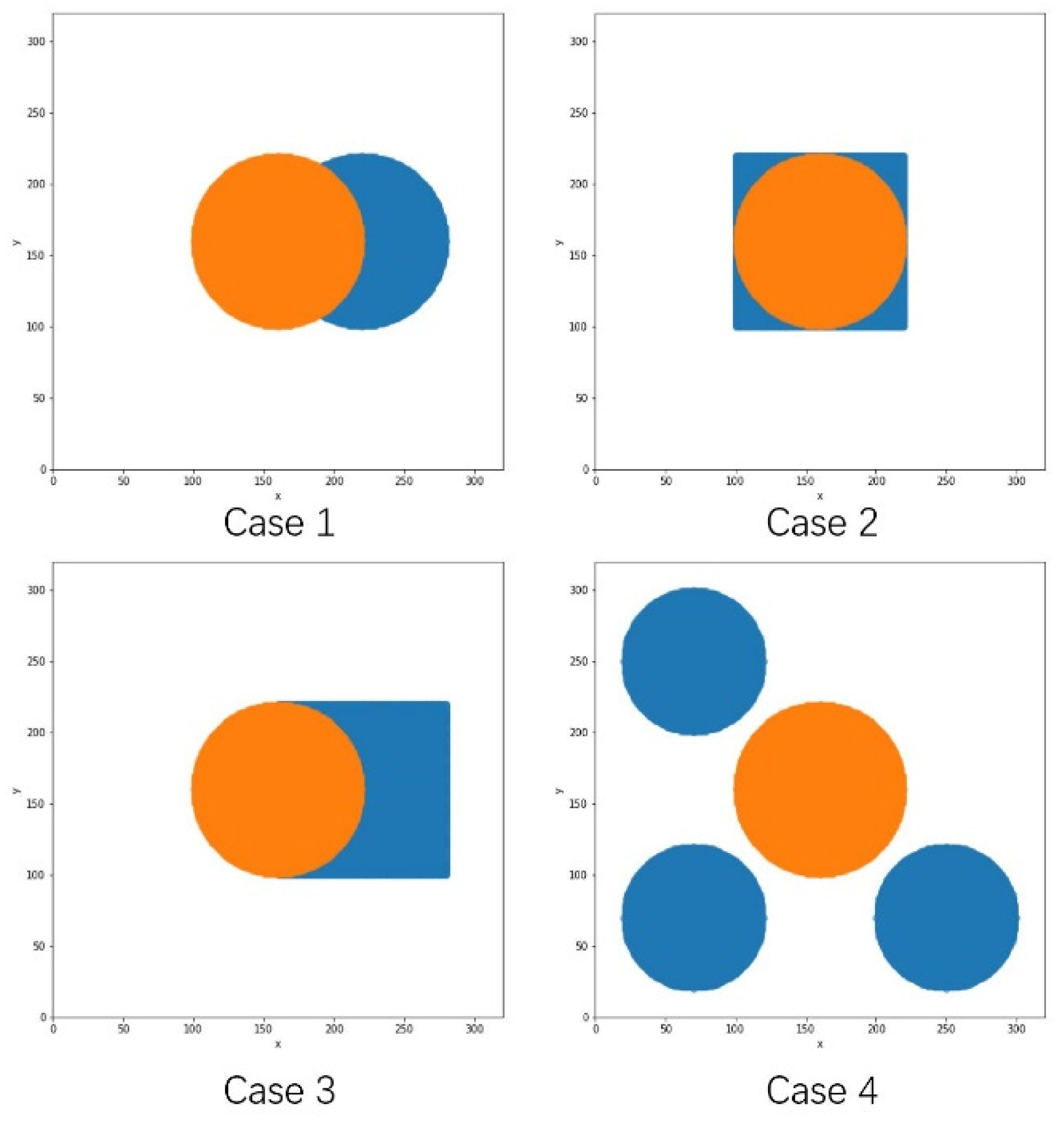
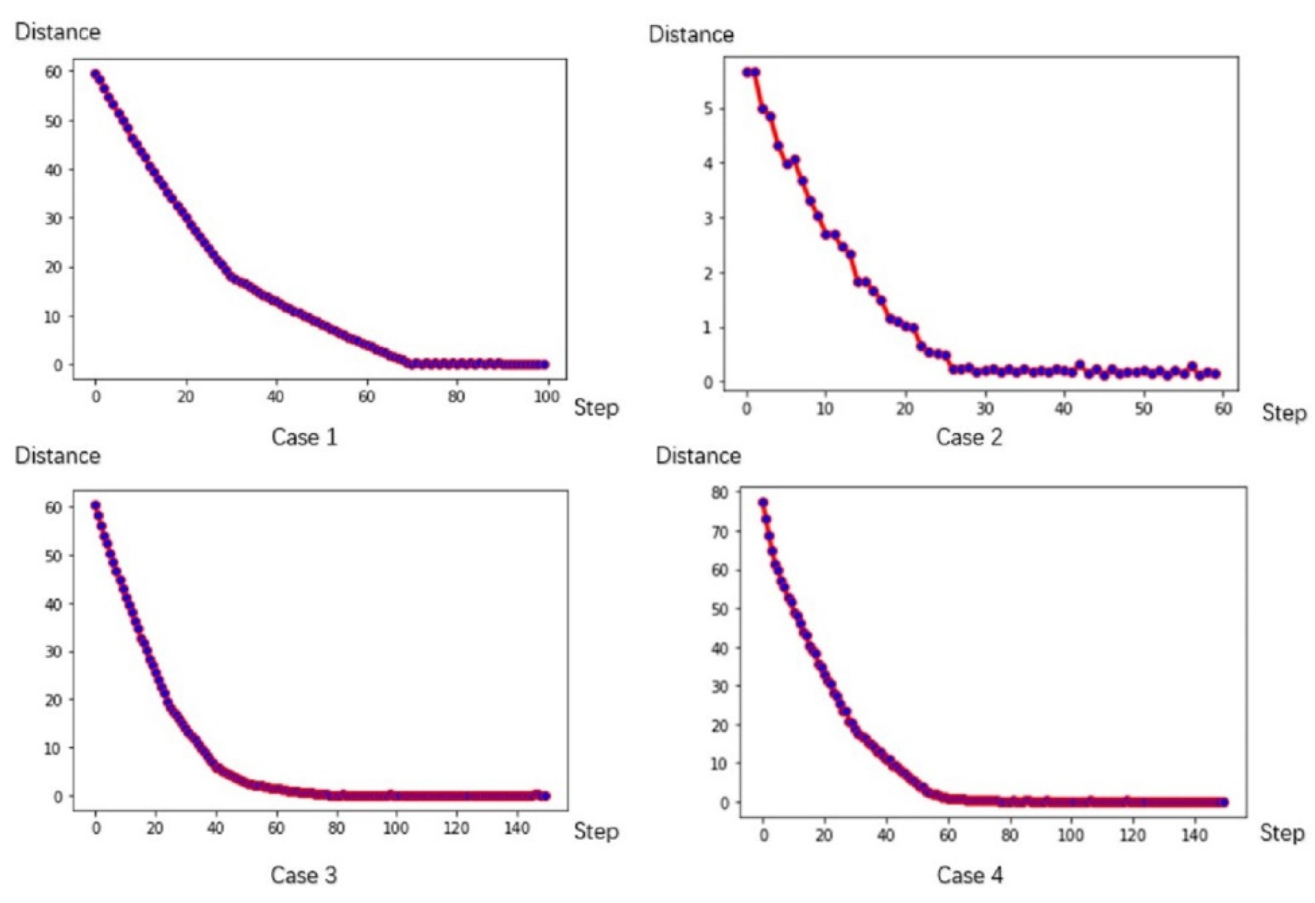
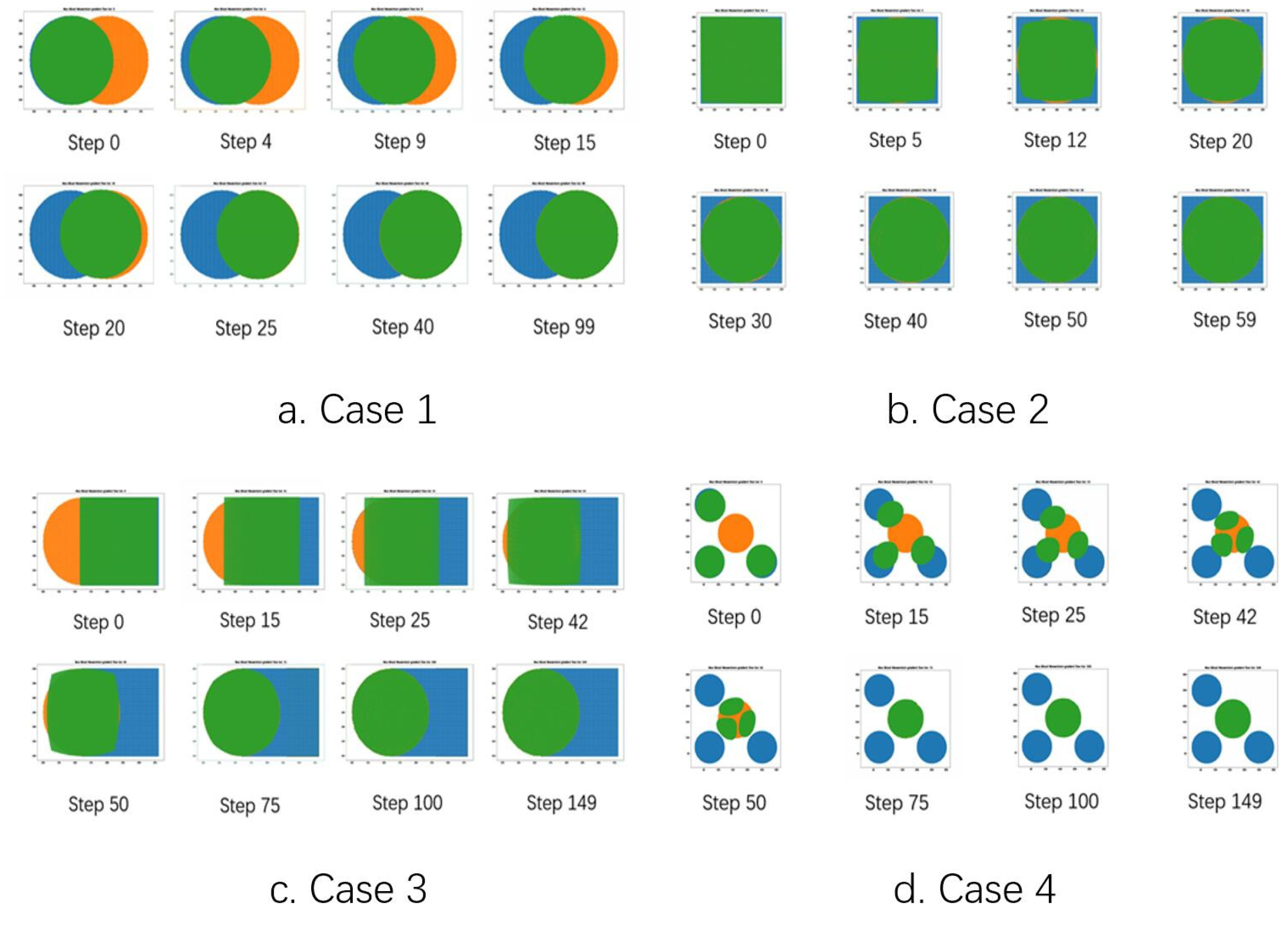
Max-sliced Wasserstein distance between areas

The geometric shape and spatial position difference between point sets (usually represented as polygons in a raster dataset) cannot be simply measured by the Euclidean distance between points. Here, we design four cases to illustrate the rationality of the proposed index:

Case 1: Shapes of the polygons in two datasets to be compared are the same, and the spatial position has a translation transformation;

Case 2: The centroid of polygons is the same, but the shapes are different;

Case 3: The polygon shapes and spatial positions are both different;

Case 4: The distribution is not continuous and there are multiple areas.

Then, we used the gradient descent method to construct the continuous transformation process.

The initial states of the four examples are shown in

Table 3. Initial state of four cases.

Case.	Distribution		Centroid		Radius/Side Length
	A	B	A	B	A	B
1	Circle	Circle	(160,160)	(220,160)	60	60
2	Circle	Square	(160,160)	(160,160)	60	60
3	Circle	Square	(160,160)	(220,160)	60	60
4	3 Circles	Circle	(70,70),(70,250),(250,70)	(160,160)	50	60

and Figure 3.

The projection number is set to 20, and then the max-sliced Wasserstein distances of each case are shown in

Table 4. Max-sliced Wasserstein distance of four cases.

Case	1	2	3	4
Distance	59.9964	5.6467	61.2305	77.3263

.

Distance changes during the gradient descent process are shown in Figure 4. As the number of iterations increases, the distance tends to decrease, which means that distribution is shifted to the target distribution.

The process of continuous transformation of four cases in the gradient descent process is shown in Figure 5.

In Case 1, the shapes of the two polygons are the same, and the max-sliced Wasserstein distance measures their difference in spatial position. When it goes to the 99th step, the initial distribution is transferred to the target distribution (the green circle moves to the same position as the orange circle).

In Case 2, the positions of the two centroids are the same, so the factor that affects the max-sliced Wasserstein distance measurement is only their geometric shapes.

In Case 3, both their geometric shapes and spatial positions affect the final measurement, so compared with that in Case 1 and Case 2, the distance is the largest.

In Case 4, the distribution of the points is discontinuous, and there are multiple parts (blue points). This simulates a more complicated situation in raster datasets. This metric gives a reasonable result and a continuous transformation process of multiple regions.

4.2. Experiments on Real Remote Sensing Products

We choose open-source global land-use raster datasets to verify the proposed index, and the three selected datasets are GLC_FCS30 [28], FROM_GLC [29], CNLUCC [30] in 2015.

The selected area is a rectangle with the coordinates range of (116.18575, 40.00125) and (116.37300, 40.18375) in the coordinate system of WGS84. The three datasets are the land-use data of this area at the same time (2015), created by different researchers, with the same resolution of 30 m.

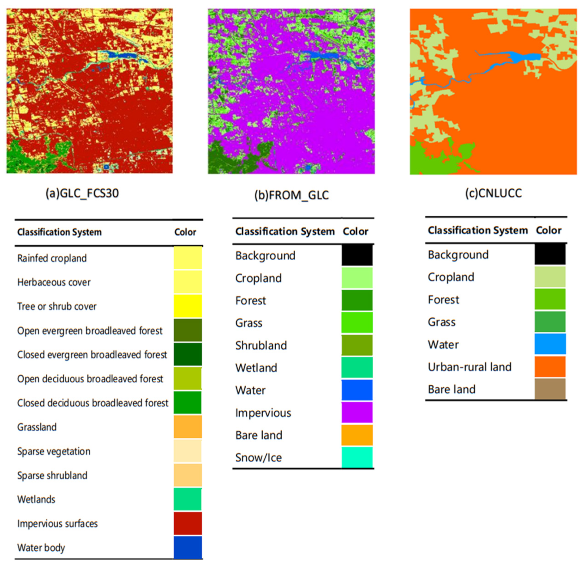
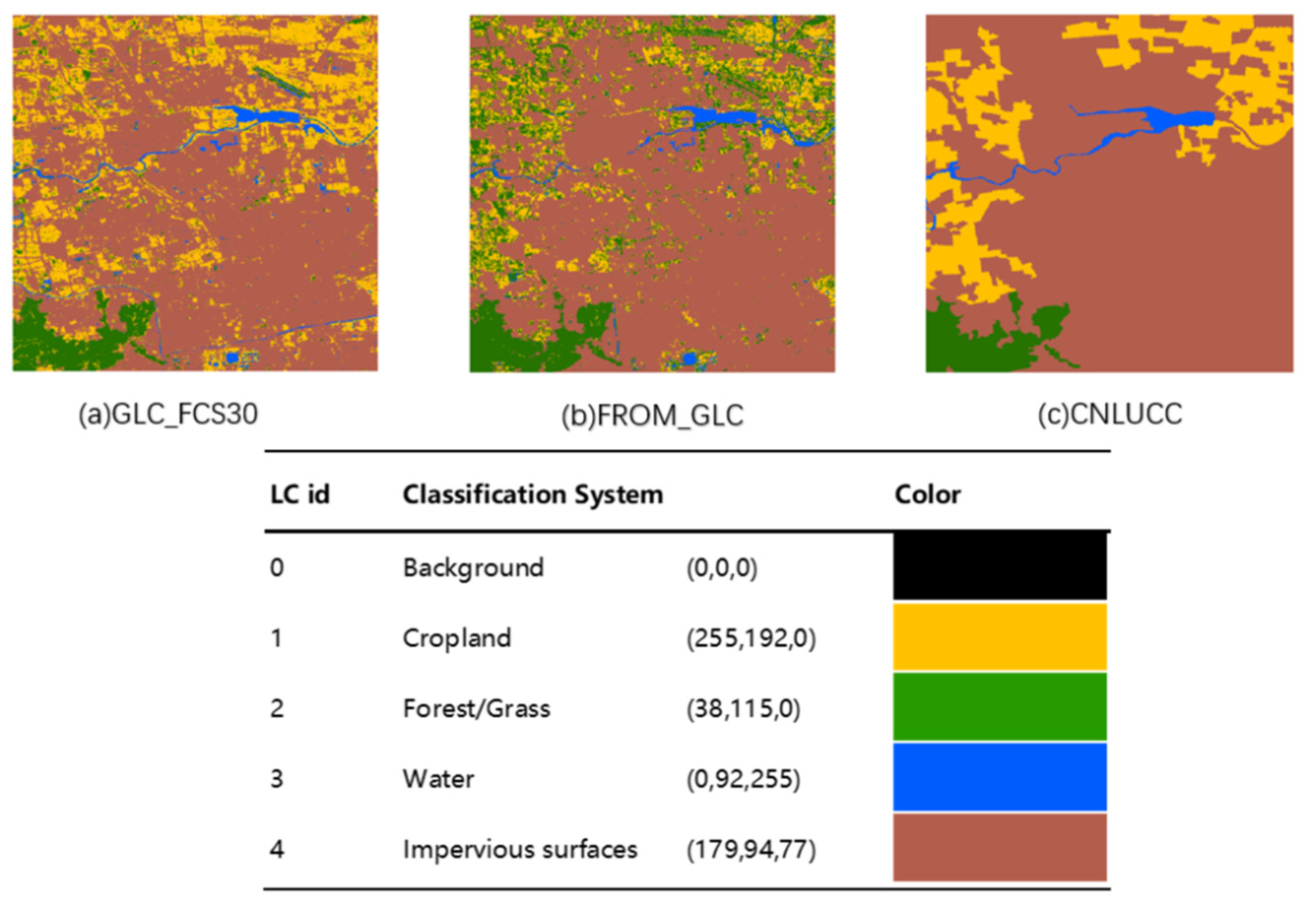
4.2.1. Dataset Preprocessing

The classification systems of the three datasets are shown in Figure 6:

Comparisons cannot be made under the original non-uniform classification system, so we reclassified the pixels and classified them into four types:(1) Cropland; (2) Forest/Grass; (3) Water body; (4) Impervious surfaces. Figure 7 illustrates the classification system and reclassification results.

Table 5. The number of pixels of four types.

	Cropland	Forest/Grass	Water	Impervious Surfaces	Total
GLC_FCS30	123,957	39,076	12,966	370,771	546,770
FROM_GLC	73,795	92,438	11,936	368,601	546,770
CNLUCC	95,176	26,149	8522	416,923	546,770

shows the pixel numbers of four classification types in each dataset.

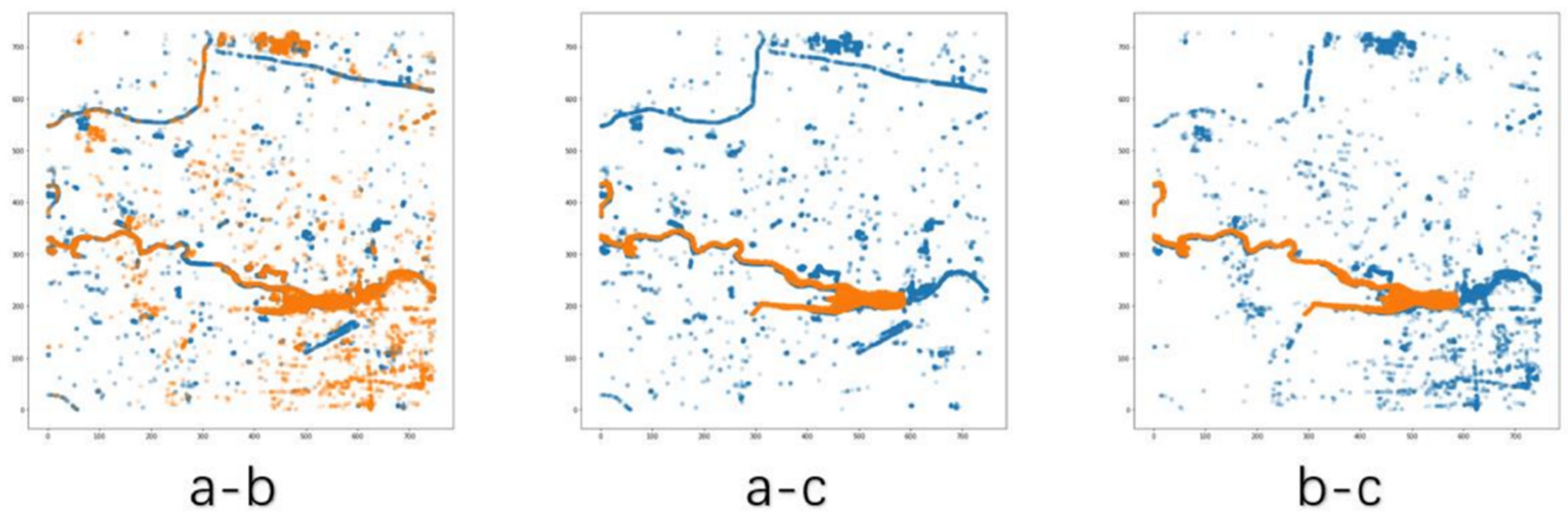
4.2.2. Similarity Calculation

Taking water bodies as an example, distributions of water bodies on the three datasets are shown in Figure 8.

Compare the three datasets in pairs separately to calculate the max-sliced Wasserstein distance of the water distribution (Figure 9 and

Table 6. Results of water body.

	Distance	Row × Col	Similarity
a-b	86.9853	749 × 730	91.49%
a-c	180.1471	749 × 730	82.43%
b-c	153.8637	749 × 730	85.01%

):

The results show that the comparison between GLC_FCS30 and FROM_GLC products (a-b) has the smallest max-sliced Wasserstein distance and thus, the highest similarity, which is consistent with the visual judgment.

The multi-category comparison results among the three chosen products are listed in

Table 7. Results of three datasets.

		a-b	a-c	b-c
Cropland	Distance	26.9367	93.0022	71.9183
	Similarity	96.85%	88.88%	91.87%
Forest/Grass	Distance	232.7238	260.1100	423.1698
	Similarity	74.71%	72.11%	54.62%
Water	Distance	86.9853	180.1471	153.8637
	Similarity	91.49%	82.43%	85.01%
Impervious	Distance	13.4117	9.71133	15.3557
surfaces	Similarity	96.04%	96.68%	94.79%
Total Similarity		93.51%	96.89%	89.80%

:

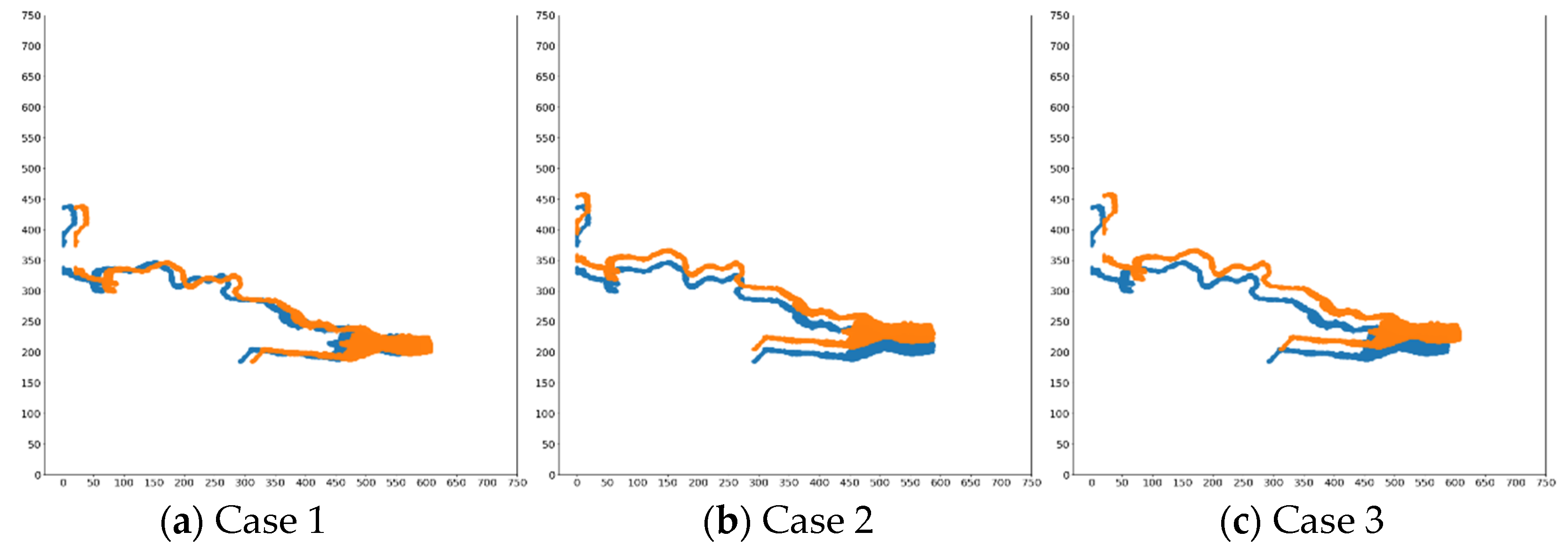
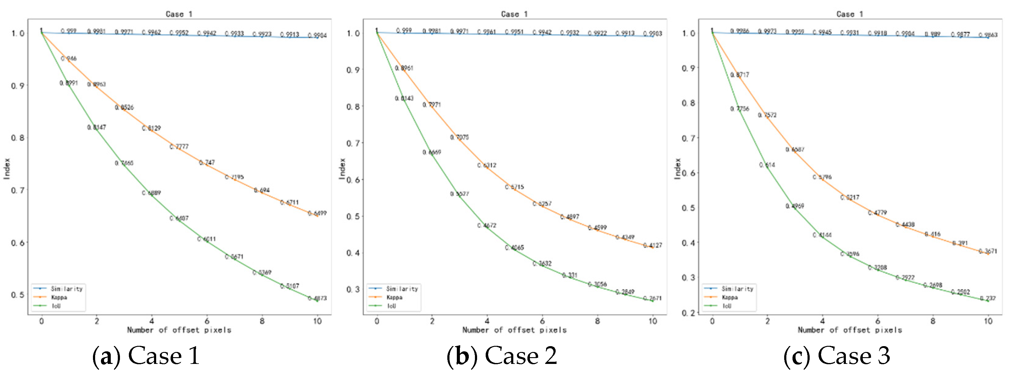
4.2.3. Comparison in Unregistered Case

We designed an experiment to illustrate a significant advantage of the proposed similarity index: it pays more attention to the shape and structure of spatial distribution than traditional methods, therefore, it can better represent the spatial features of data. We simulated a misregistered case of a water body in CNLUCC data. Cases 1–3 offset 1 to 20 pixels on the x-axis, y-axis, x- and y-axis, respectively (Figure 10), and then we calculated according to the similarity index, kappa coefficient and intersection over union (IoU). The results are shown in

Table 8. Similarity, Kappa and IoU results of three unregistered cases.

Offset Pixel	Case 1			Case 2			Case 3
	Similarity	Kappa	IoU	Similarity	Kappa	IoU	Similarity	Kappa	IoU
1	0.9990	0.9460	0.8991	0.999	0.8961	0.8143	0.9986	0.8717	0.7756
2	0.9981	0.8963	0.8147	0.9981	0.7971	0.6669	0.9973	0.7572	0.6140
3	0.9971	0.8526	0.7465	0.9971	0.7075	0.5527	0.9959	0.6587	0.4969
4	0.9962	0.8129	0.6889	0.9961	0.6312	0.4672	0.9945	0.5796	0.4144
5	0.9952	0.7777	0.6407	0.9951	0.5715	0.4065	0.9931	0.5217	0.3596
6	0.9942	0.7470	0.6011	0.9942	0.5257	0.3632	0.9918	0.4779	0.3208
7	0.9933	0.7195	0.5671	0.9932	0.4897	0.3310	0.9904	0.4438	0.2922
8	0.9923	0.6940	0.5369	0.9922	0.4599	0.3056	0.989	0.416	0.2698
9	0.9913	0.6711	0.5107	0.9913	0.4349	0.2849	0.9877	0.391	0.2502
10	0.9904	0.6499	0.4873	0.9903	0.4127	0.2671	0.9863	0.3671	0.2320

.

It could be seen that traditional methods are very sensitive to registration accuracy (shown in Figure 11).

Both the kappa coefficient and IoU are not robust in three cases, because these methods do not consider spatial features of pixels; therefore, their results are quite different in cases of different pixel offsets. The similarity index proposed in this paper focuses on the structure and characteristics of space, thus, the max-sliced Wasserstein distance is close to the true pixel offset and the change of similarity result is small.

5. Discussion

In the above experiments, test datasets are used to illustrate the rationality of Wasserstein distance for quantitatively calculating the distribution of pixels in two-dimensional space. This index can comprehensively consider spatial location information and geometric shape information, which has practical significance.

After unifying the spatial resolution and classification standards of three chosen land cover products, single-category similarity and overall similarity are both calculated. In the calculation of water body similarity, the distribution of large-area water objects in products GLC_FCS30 and FROM_GLC is relatively consistent, and the difference in the surrounding scattered and small water bodies is the main reason for the generation of the distance measurement. The overall similarity results indicate that the GLC_FCS30 and CNLUCC data have a higher similarity. This is because, in FROM_GLC, the confusion between Cropland and Forest/Grass types appears more frequently, resulting in a large gap in the number of pixels between these two types. Therefore, after calculating the overall similarity with the number of pixels and similarity in the similarity evaluation index, the overall similarity is quite different from the other two products. The most similar type is Impervious surfaces, and the pixels of this type account for a large proportion of the total number of pixels, therefore, it is the main factor that affects the final similarity.

Compared with the error matrix and IoU, the similarity index represents more characteristics of spatial structure. We hope to propose this index to make up for the shortcomings of existing methods. It can better characterize the spatial relationship between datasets and solve the comparison problem under a certain degree of misregistration.

6. Conclusions

With the increasing demand for quantitative evaluation of different remote sensing products, the traditional pixel-based accuracy evaluation system needs to be improved. The proposed similarity index is a promising way to facilitate this need. It is not limited to pixel-by-pixel comparison in the case of complete alignment. In a word, the main idea of this study is to transform the relative accuracy comparison problem of multi-source raster datasets into an optimal transmission problem in two-dimensional space. For the mathematical expression of similarity index, based on max-sliced Wasserstein distance, when the number of projections reaches the threshold, it can be regarded as the true value. Using the gradient descent method to give the continuous transformation process also shows that the index can reasonably quantify the spatial distribution. Based on this similarity index, the spatial difference between multi-source raster datasets can be quantified. Theoretically, this index is more suitable for land-use change monitoring and continuous raster datasets comparison. More theoretical development and practical application of this index are still under work, and we will continue to improve it.

References

1. Hansen, M.C.; Reed, B. A comparison of the IGBP DISCover and University of Maryland 1 km global land cover products. Int. J. Remote Sens. 2000, 21, 1365–1373. [Google Scholar] [CrossRef]
2. Zhu, Z.; Waller, E. Global forest cover mapping for the United Nations Food and Agriculture Organization forest resources assessment 2000 program. For. Sci. 2003, 49, 369–380. [Google Scholar]
3. Stehman, S.V. Sampling designs for accuracy assessment of land cover. Int. J. Remote Sens. 2009, 30, 5243–5272. [Google Scholar] [CrossRef]
4. Visser, H.; Nijs, T.D. The Map Comparison Kit. Environ. Model. Softw. 2006, 21, 346–358. [Google Scholar] [CrossRef]
5. Ma, Z.; Redmond, R.L. Tau coefficients for accuracy assessment of classification of remote sensing data. Photogramm. Eng. Remote Sens. 1995, 61, 435–439. [Google Scholar]
6. Pontius, R., Jr.; Huffaker, D.; Denman, K. Useful techniques of validation for spatially explicit land-change models. Ecol. Model. 2004, 179, 445–461. [Google Scholar] [CrossRef]
7. Rees, W.G. Comparing the spatial content of thematic maps. Int. J. Remote Sens. 2008, 29, 3833–3844. [Google Scholar] [CrossRef]
8. Wu, B.; Zhang, L.; Zhao, Y. Feature selection via Cramer’s V-test discretization for remote-sensing image classification. IEEE Trans. Geosci. Remote Sens. 2013, 52, 2593–2606. [Google Scholar] [CrossRef]
9. Ohana-Levi, N.; Gao, F.; Knipper, K.; Kustas, W.P.; Anderson, M.C.; del Mar Alsina, M.; Sanchez, L.A.; Karnieli, A. Time-series clustering of remote sensing retrievals for defining management zones in a vineyard. Irrig. Sci. 2021, 1–15. [Google Scholar] [CrossRef]
10. Hagen-Zanker, A. Map comparison methods that simultaneously address overlap and structure. J. Geogr. Syst. 2006, 8, 165–185. [Google Scholar] [CrossRef]
11. San-Miguel-Ayanz, G.H. Conventional and fuzzy comparisons of large scale land cover products: Application to CORINE, GLC2000, MODIS and GlobCover in Europe. ISPRS J. Photogramm. Remote Sens. 2012, 74, 185–201. [Google Scholar]
12. Dou, W.; Ren, Y.; Wu, Q.; Ruan, S.; Chen, Y.; Bloyet, D.; Constans, J.M. Fuzzy kappa for the agreement measure of fuzzy classifications. Neurocomputing 2007, 70, 726–734. [Google Scholar] [CrossRef] [Green Version]
13. Hargrove, W.W.; Hoffman, F.M.; Hessburg, P.F. Mapcurves: A quantitative method for comparing categorical maps. J. Geogr. Syst. 2006, 8, 187. [Google Scholar] [CrossRef]
14. White, R. Pattern based map comparisons. J. Geogr. Syst. 2006, 8, 145–164. [Google Scholar] [CrossRef]
15. Zhu, D.; Chen, T.; Wang, Z.; Niu, R. Detecting ecological spatial-temporal changes by remote sensing ecological index with local adaptability. J. Environ. Manag. 2021, 299, 113655. [Google Scholar] [CrossRef]
16. Giri, C.; Zhu, Z.; Reed, B. A comparative analysis of the Global Land Cover 2000 and MODIS land cover data sets. Remote Sens. Environ. 2005, 94, 123–132. [Google Scholar] [CrossRef]
17. Strahler, A.H.; Boschetti, L.; Foody, G.M.; Friedl, M.A.; Hansen, M.C.; Herold, M.; Mayaux, P.; Morisette, J.T.; Stehman, S.V.; Woodcock, C.E. Global Land Cover Validation: Recommendations for Evaluation and Accuracy Assessment of Global Land Cover Maps. Eur. Communities Luxemb. 2006, 51, 1–60. [Google Scholar]
18. Foody, G.M. Assessing the accuracy of land cover change with imperfect ground reference data. Remote Sens. Environ. 2010, 114, 2271–2285. [Google Scholar] [CrossRef] [Green Version]
19. Foody, G.M. Explaining the unsuitability of the kappa coefficient in the assessment and comparison of the accuracy of thematic maps obtained by image classification. Remote Sens. Environ. 2020, 239, 111630. [Google Scholar] [CrossRef]
20. Enøe, C.; Georgiadis, M.P.; Johnson, W.O. Estimation of sensitivity and specificity of diagnostic tests and disease prevalence when the true disease state is unknown. Prev. Vet. Med. 2000, 45, 61–81. [Google Scholar] [CrossRef]
21. Wu, X.; Naegeli, K.; Wunderle, S. Geometric accuracy assessment of coarse-resolution satellite datasets: A study based on AVHRR GAC data at the sub-pixel level. Earth Syst. Sci. Data 2020, 12, 539–553. [Google Scholar] [CrossRef] [Green Version]
22. Wang, H.; Skau, E.; Krim, H.; Cervone, G. Fusing heterogeneous data: A case for remote sensing and social media. IEEE Trans. Geosci. Remote Sens. 2018, 56, 6956–6968. [Google Scholar] [CrossRef]
23. Tardy, B.; Inglada, J.; Michel, J. Assessment of optimal transport for operational land-cover mapping using high-resolution satellite images time series without reference data of the mapping period. Remote Sens. 2019, 11, 1047. [Google Scholar] [CrossRef] [Green Version]
24. Deshpande, I.; Hu, Y.T.; Sun, R.; Pyrros, A.; Schwing, A. Max-Sliced Wasserstein Distance and its use for GANs. In Proceedings of the 2019 IEEE/CVF International Conference on Computer Vision Workshop, Seoul, Korea, 27–28 October 2019; pp. 10648–10656. [Google Scholar]
25. Gulrajani, I.; Ahmed, F.; Arjovsky, M.; Dumoulin, V.; Courville, A. Improved training of wasserstein gans. arXiv Prepr. 2017, arXiv:1704.00028. [Google Scholar]
26. Kolouri, S.; Rohde, G.K.; Hoffmann, H. Sliced wasserstein distance for learning gaussian mixture models. In Proceedings of the IEEE Conference on Computer Vision and Pattern Recognition, Salt Lake City, UT, USA, 18–23 June 2018; pp. 3427–3436. [Google Scholar]
27. Kolouri, S.; Park, S.R.; Rohde, G.K. The radon cumulative distribution transform and its application to image classification. IEEE Trans. Image Processing 2015, 25, 920–934. [Google Scholar] [CrossRef]
28. Zhang, X.; Liu, L.; Chen, X.; Gao, Y.; Xie, S.; Mi, J. GLC_FCS30: Global land-cover product with fine classification system at 30 m using time-series Landsat imagery. Earth Syst. Sci. Data 2021, 13, 2753–2776. [Google Scholar] [CrossRef]
29. Gong, P.; Wang, J.; Yu, L.; Zhao, Y.; Chen, J. Finer resolution observation and monitoring of global land cover: First mapping results with Landsat TM and ETM+ data. Int. J. Remote Sens. 2013, 34, 48. [Google Scholar] [CrossRef] [Green Version]
30. Xu, X.; Liu, J.; Zhang, S.; Li, R.; Yan, C.; Wu, S. China’s Multi-Period Land Use Land Cover Remote Sensing Monitoring Data Set (CNLUCC); Resource and Environment Data Cloud Platform: Beijing, China, 2018. [Google Scholar]
Figure 1. Three datasets of water body distribution (areas with differences are circled in red).
Remotesensing 14 02546 g001
Figure 2. Optimal transport problems: (a) one-dimensional case; (b) two-dimensional case.
Remotesensing 14 02546 g002
Figure 3. Initial state of four cases.
Remotesensing 14 02546 g003
Figure 4. Distance with steps.
Remotesensing 14 02546 g004
Figure 5. Transformation process of source distribution to target.
Remotesensing 14 02546 g005
Figure 6. Detail of GLC_FCS30, FROM_GLC and CNLUCC datasets.
Remotesensing 14 02546 g006
Figure 7. Classification System and results of reclassification.
Remotesensing 14 02546 g007
Figure 8. Water body distribution. (a) GLC_FCS30; (b) FROM_GLC; (c) CNLUCC.
Remotesensing 14 02546 g008
Figure 9. Overlay of raster data map frames (a-b. GLC_FCS30-FROM_GLC; a-c. GLC_FCS30-CNLUCC; b-c. FROM_GLC-CNLUCC).
Remotesensing 14 02546 g009
Figure 10. Unregistered cases (Case 1: x-axis; Case 2: y-axis; Case 3: both).
Remotesensing 14 02546 g010
Figure 11. Line charts of three indicators changes with pixel offset.
Remotesensing 14 02546 g011