Figure 1.
Different strategies of input: (a) the overlapping original information strategy, (b) the overlapping high-pass information strategy, and (c) the differential information mapping strategy.
Figure 1.
Different strategies of input: (a) the overlapping original information strategy, (b) the overlapping high-pass information strategy, and (c) the differential information mapping strategy.
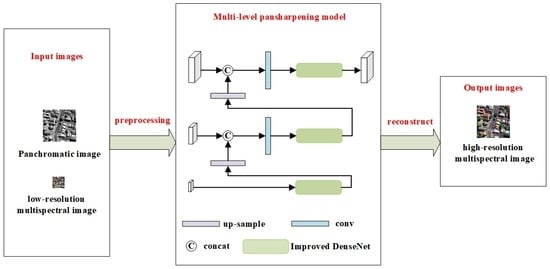
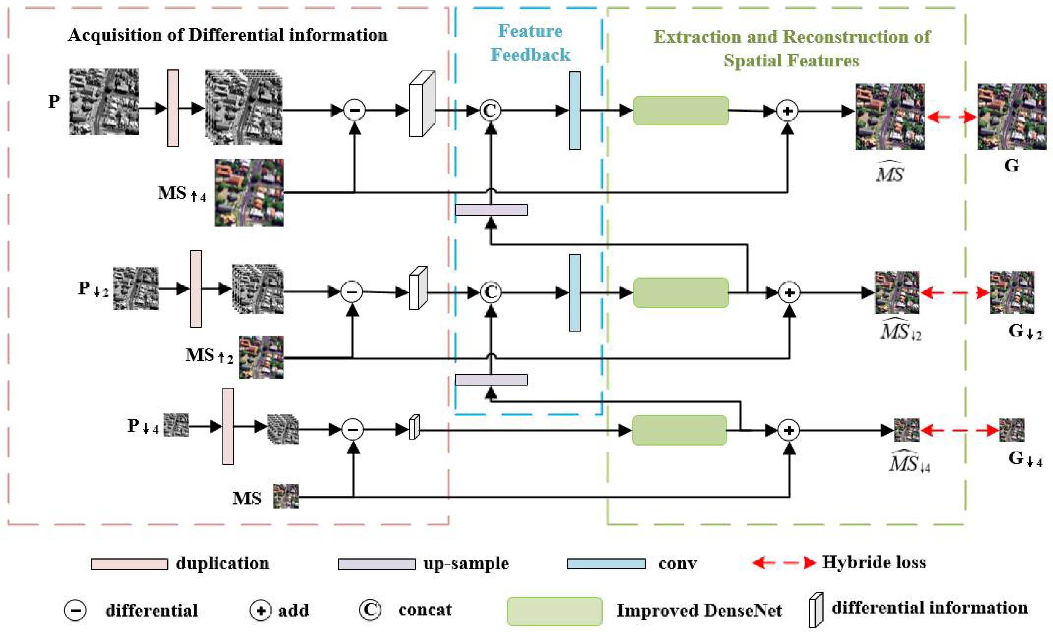
Figure 2.
The framework of the proposed DS-MDNP.
Figure 2.
The framework of the proposed DS-MDNP.
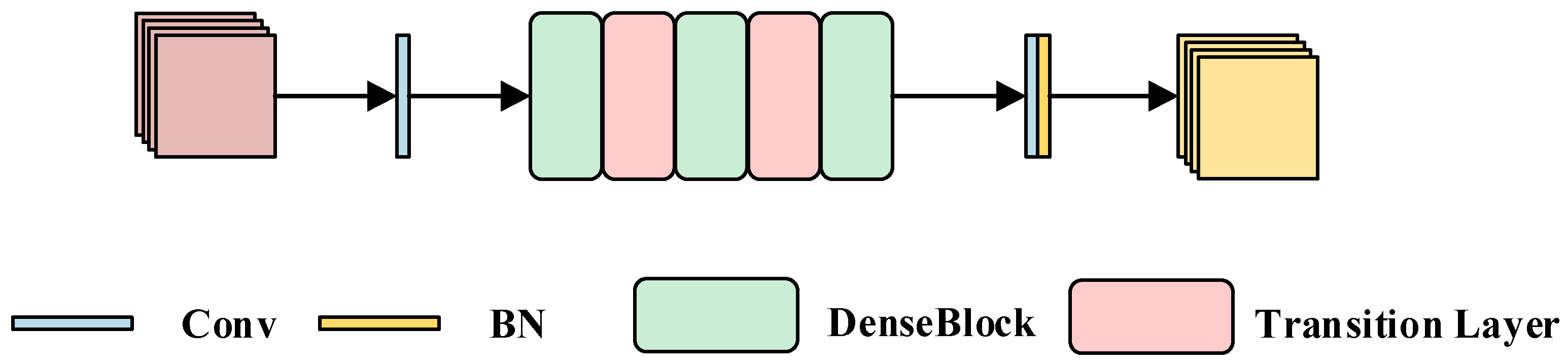
Figure 3.
The framework of improved DenseNet.
Figure 3.
The framework of improved DenseNet.
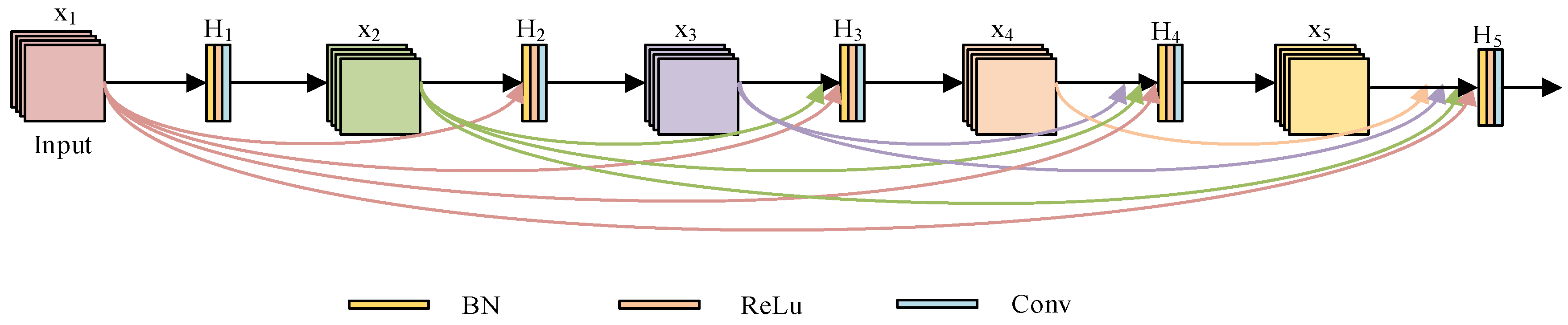
Figure 4.
Architecture of DenseBlock.
Figure 4.
Architecture of DenseBlock.
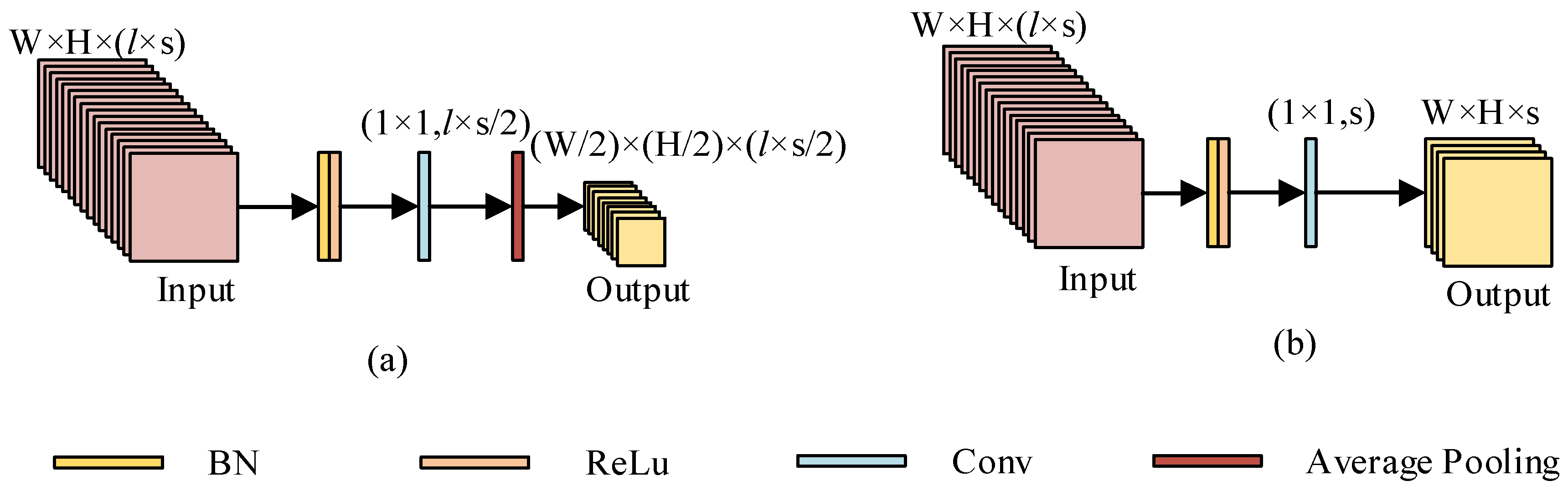
Figure 5.
The transition layers: (a) the traditional transition layer and (b) the improved transition layer.
Figure 5.
The transition layers: (a) the traditional transition layer and (b) the improved transition layer.
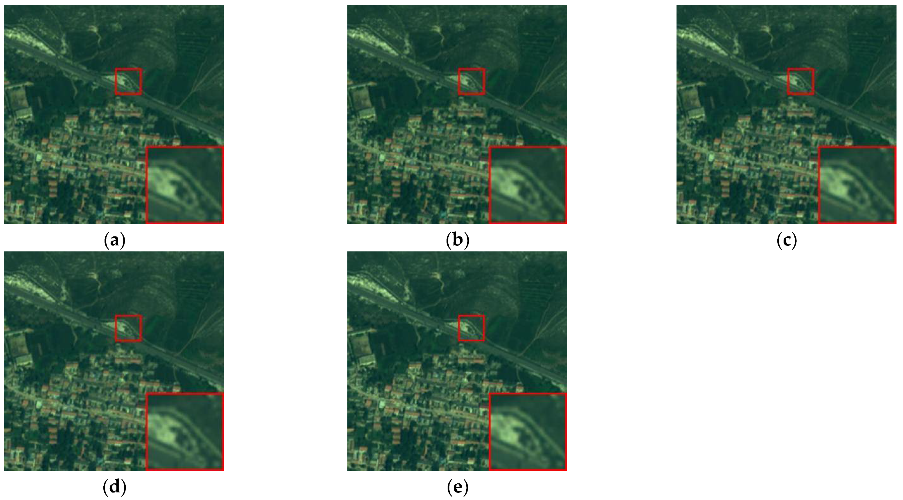
Figure 6.
Fused image of WorldView-2. (a) Base line, (b) differential, (c) DenseNet, (d) differential + DenseNet, (e) differential + DenseNet + Hybrid Loss.
Figure 6.
Fused image of WorldView-2. (a) Base line, (b) differential, (c) DenseNet, (d) differential + DenseNet, (e) differential + DenseNet + Hybrid Loss.
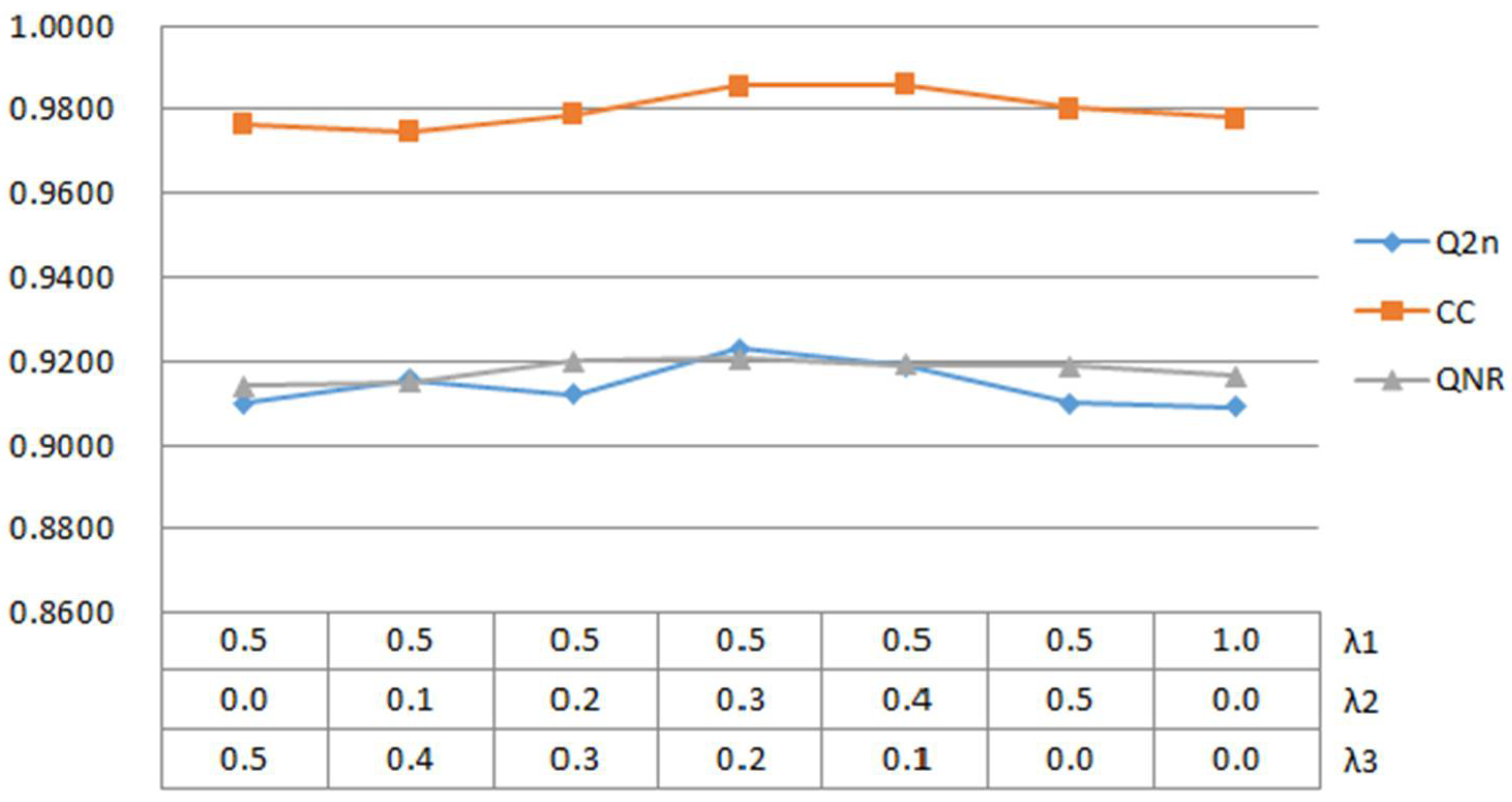
Figure 7.
Line graph for mixed loss parameter validation.
Figure 7.
Line graph for mixed loss parameter validation.
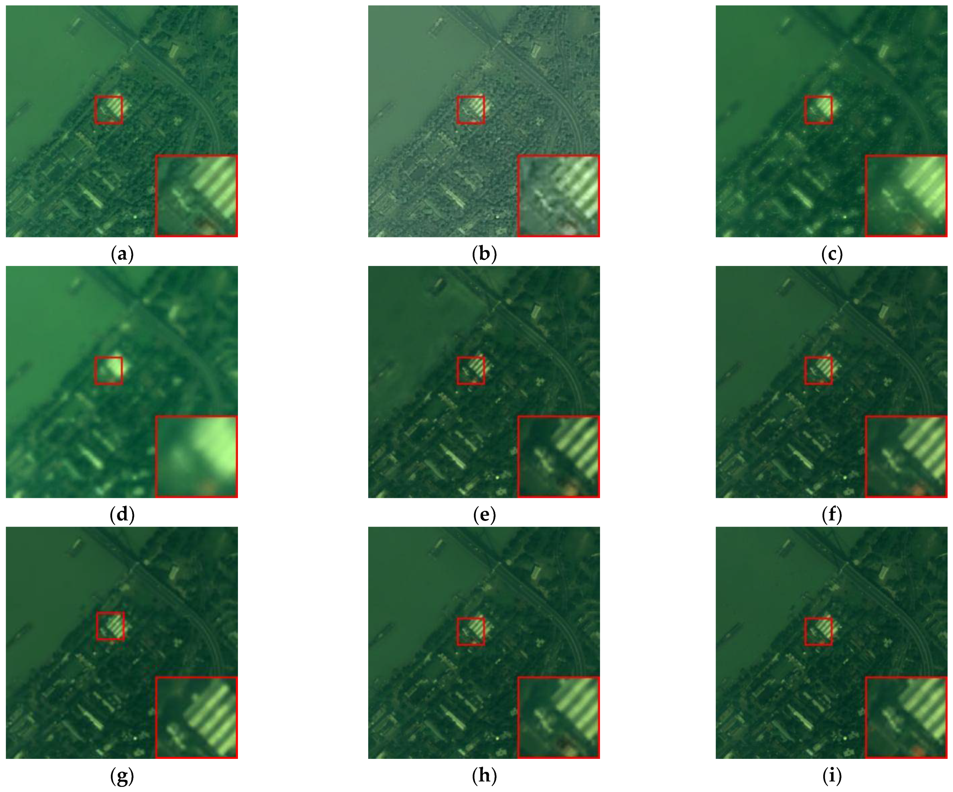
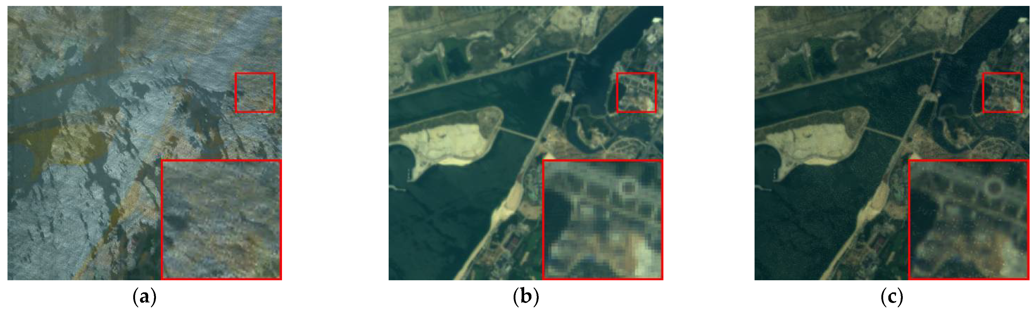
Figure 8.
Fused images of QuickBird where (a) IHS, (b) Wavelet, (c) HPF, (d) PRACS, (e) PNN, (f) Fusion-Net, (g) SSConv, (h) DS-MDNP, and (i) GT.
Figure 8.
Fused images of QuickBird where (a) IHS, (b) Wavelet, (c) HPF, (d) PRACS, (e) PNN, (f) Fusion-Net, (g) SSConv, (h) DS-MDNP, and (i) GT.
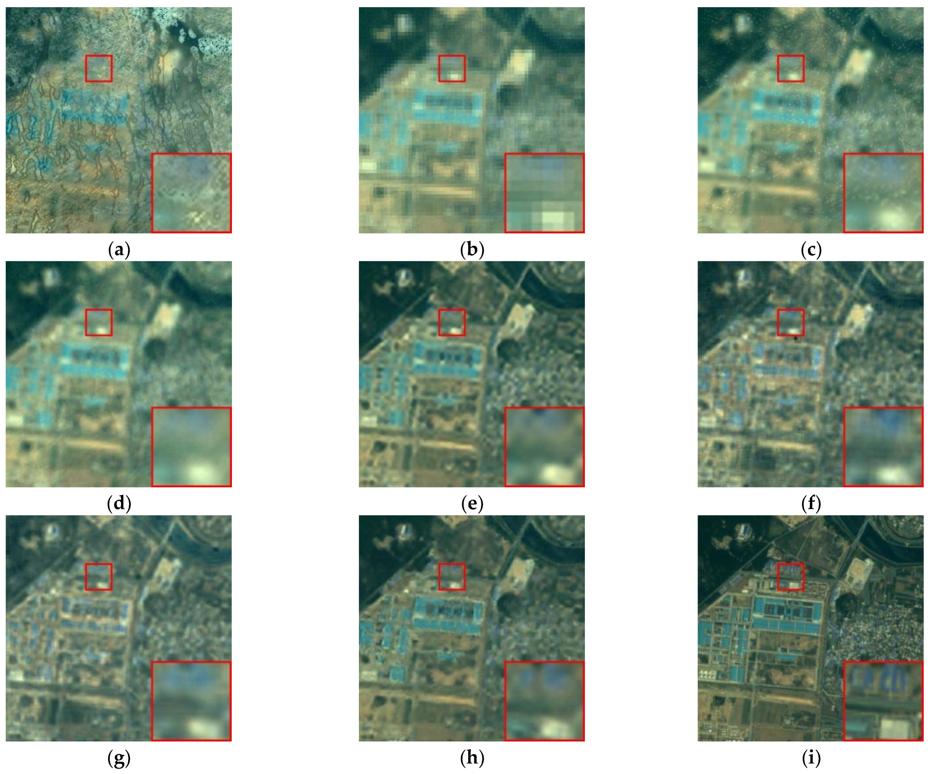
Figure 9.
The fused images of GaoFen-1 where (a) IHS, (b) Wavelet, (c) HPF, (d) PRACS, (e) PNN, (f) Fusion-Net, (g) SSConv, (h) DS-MDNP, and (i) GT.
Figure 9.
The fused images of GaoFen-1 where (a) IHS, (b) Wavelet, (c) HPF, (d) PRACS, (e) PNN, (f) Fusion-Net, (g) SSConv, (h) DS-MDNP, and (i) GT.
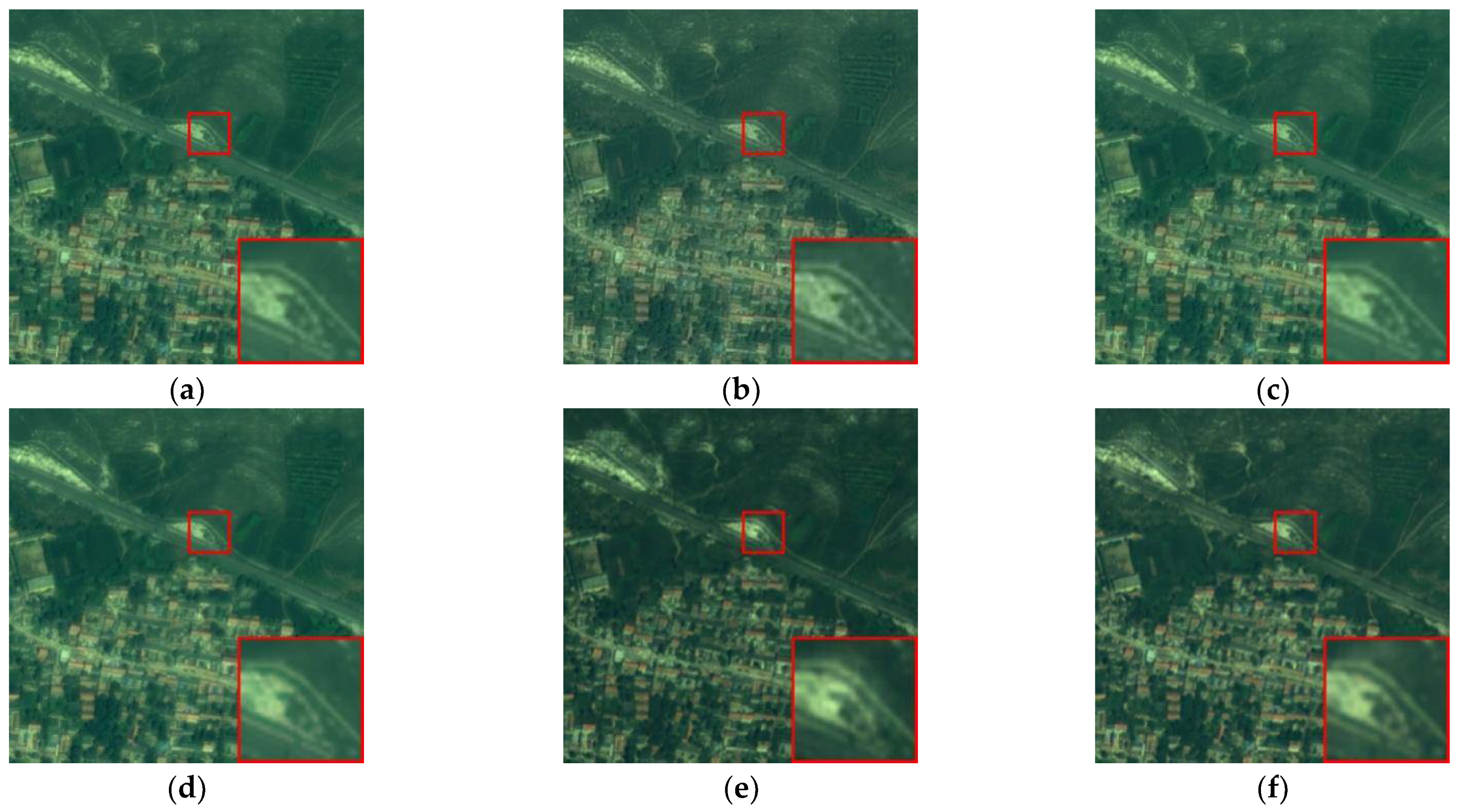
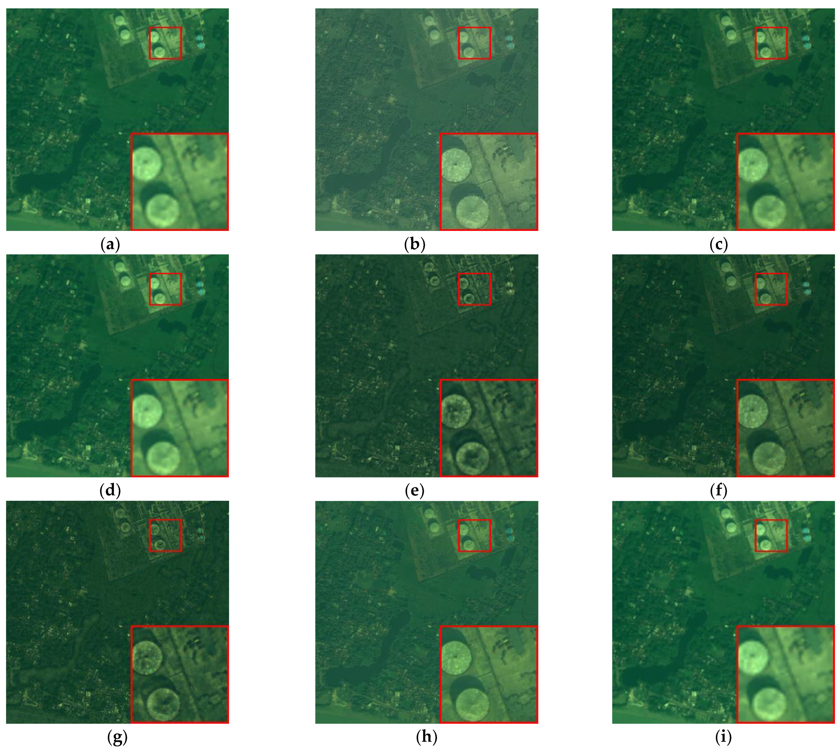
Figure 10.
Fused images of WorldView-2 where (a) IHS, (b) Wavelet, (c) HPF, (d) PRACS, (e) PNN, (f) Fusion-Net, (g) SSConv, (h) DS-MDNP, and (i) GT.
Figure 10.
Fused images of WorldView-2 where (a) IHS, (b) Wavelet, (c) HPF, (d) PRACS, (e) PNN, (f) Fusion-Net, (g) SSConv, (h) DS-MDNP, and (i) GT.
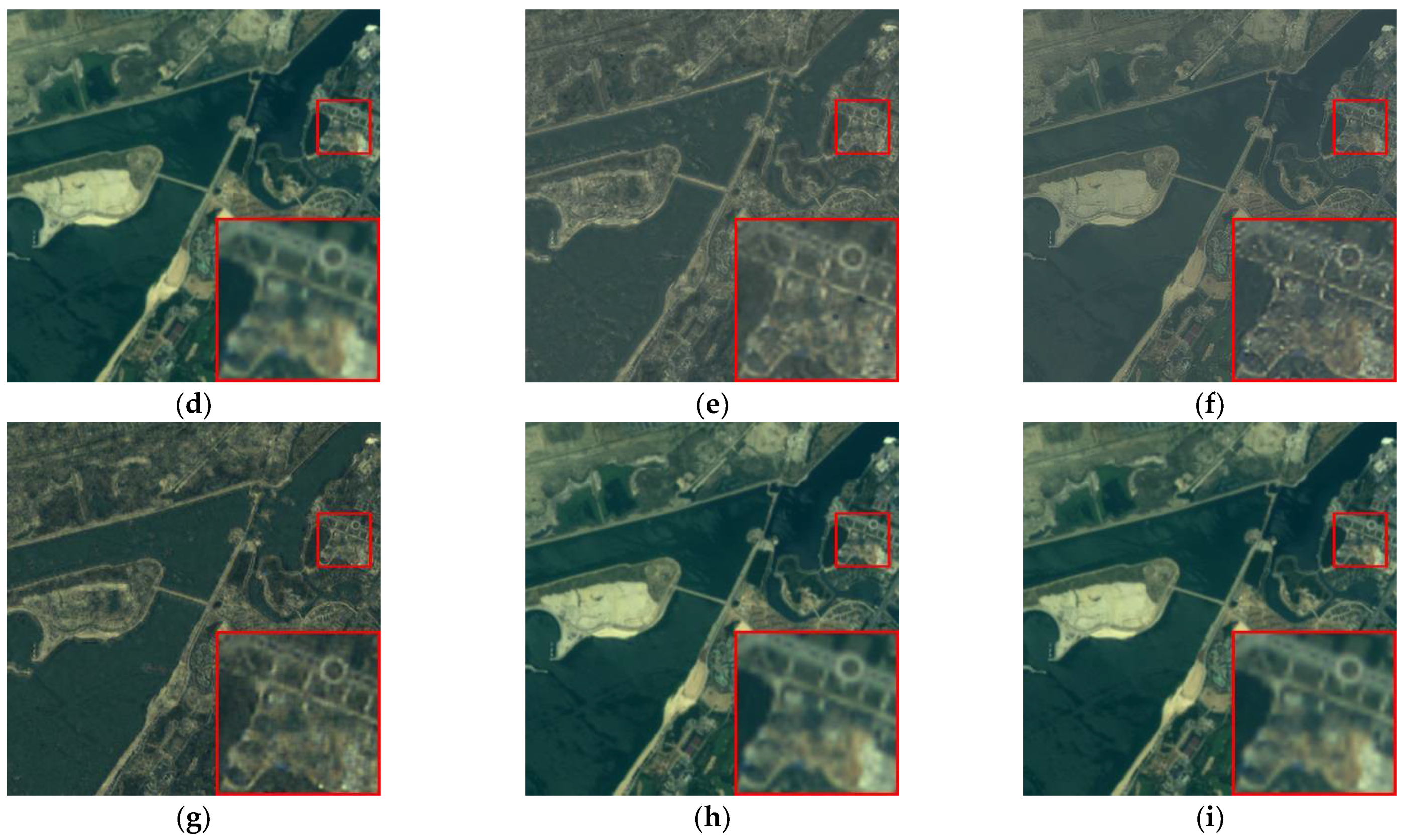
Figure 11.
Fused images of WorldView-2 where (a) IHS, (b) Wavelet, (c) HPF, (d) PRACS, (e) PNN, (f) Fusion-Net, (g) SSConv, (h) DS-MDNP, and (i) Bicubic.
Figure 11.
Fused images of WorldView-2 where (a) IHS, (b) Wavelet, (c) HPF, (d) PRACS, (e) PNN, (f) Fusion-Net, (g) SSConv, (h) DS-MDNP, and (i) Bicubic.
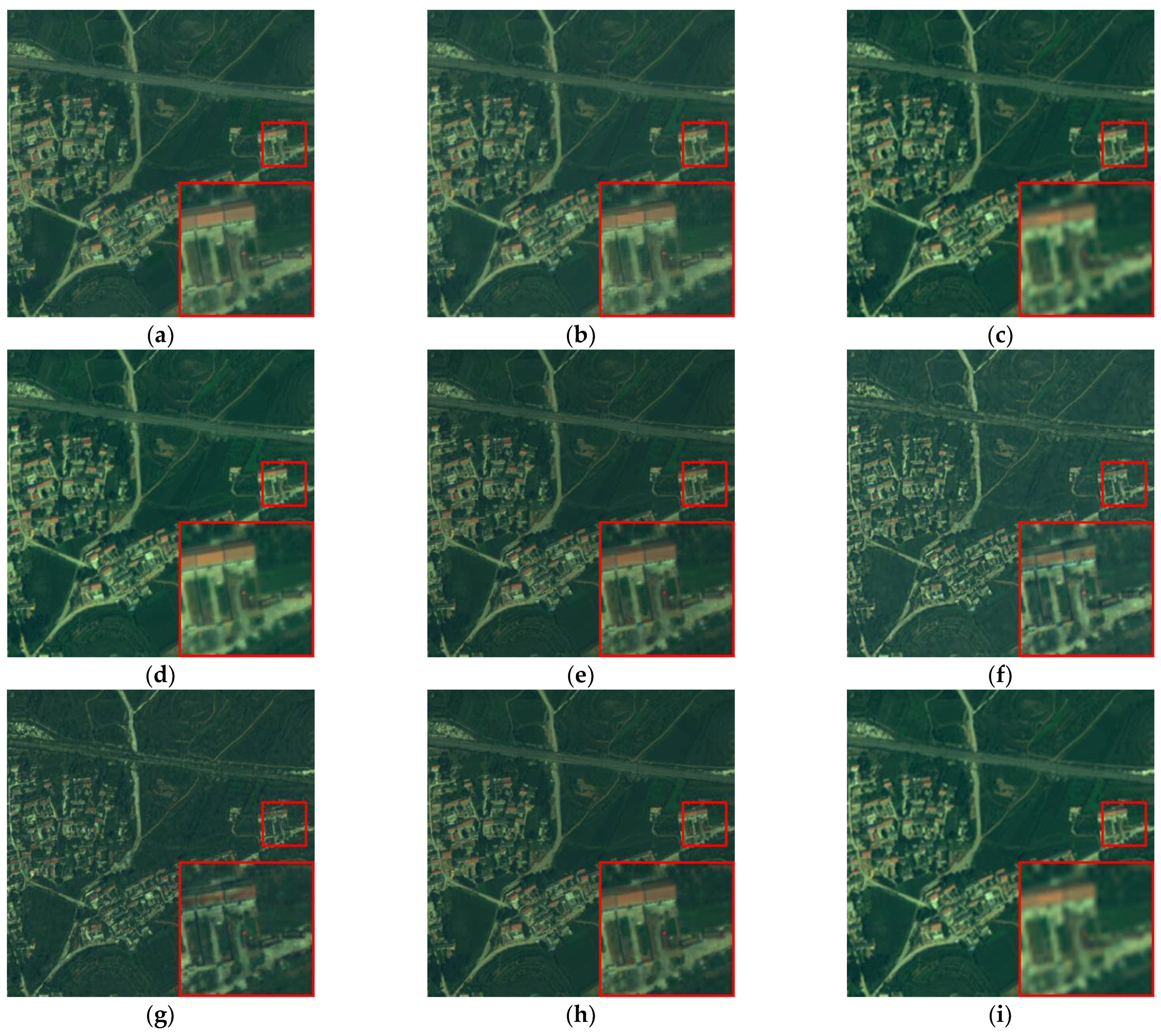
Figure 12.
Fused images of QuickBird where (a) IHS, (b) Wavelet, (c) HPF, (d) PRACS, (e) PNN, (f) Fusion-Net, (g) SSConv, (h) DS-MDNP, and (i) Bicubic.
Figure 12.
Fused images of QuickBird where (a) IHS, (b) Wavelet, (c) HPF, (d) PRACS, (e) PNN, (f) Fusion-Net, (g) SSConv, (h) DS-MDNP, and (i) Bicubic.
Figure 13.
Fused images of GaoFen-1 where (a) IHS, (b) Wavelet, (c) HPF, (d) PRACS, (e) PNN, (f) Fusion-Net, (g) SSConv, (h) DS-MDNP, and (i) Bicubic.
Figure 13.
Fused images of GaoFen-1 where (a) IHS, (b) Wavelet, (c) HPF, (d) PRACS, (e) PNN, (f) Fusion-Net, (g) SSConv, (h) DS-MDNP, and (i) Bicubic.
Table 1.
Size of training and validation sets for GaoFen-1, QuickBird, and WorldView-2.
Table 1.
Size of training and validation sets for GaoFen-1, QuickBird, and WorldView-2.
| Dataset | Training Set | Validation Set | Size of Original PAN Image | Size of Original MS Images |
|---|
| QuickBird | 2187 | 546 | 16,251 × 16,004 | 4063 × 4001 × 4 |
| GaoFen-1 | 2779 | 694 | 18,192 × 18,000 | 4548 × 4500 × 4 |
| WorldView-2 | 1603 | 400 | 16,384 × 16,384 | 4096 × 4096 × 4 |
Table 2.
Size of PAN image, MS images, and GT images for GaoFen-1, QuickBird, and WorldView-2.
Table 2.
Size of PAN image, MS images, and GT images for GaoFen-1, QuickBird, and WorldView-2.
| Dataset | PAN | MS | GT |
|---|
| QuickBird | 64 × 64 | 16 × 16 × 4 | 64 × 64 × 4 |
| GaoFen-1 | 64 × 64 | 16 × 16 × 4 | 64 × 64 × 4 |
| WorldView-2 | 64 × 64 | 16 × 16 × 4 | 64 × 64 × 4 |
Table 3.
Quantitative evaluation results of ablation experiments on the WorldView-2 dataset. The values in bold represent the best results.
Table 3.
Quantitative evaluation results of ablation experiments on the WorldView-2 dataset. The values in bold represent the best results.
| Method | Strategies | Quantitative Evaluation Indices |
|---|
| | Differential | DenseNet | Hybrid Loss | SAM | ERGAS | Q | Q2n | CC |
|---|
| 1 | | | | 3.5142 | 2.1057 | 0.9342 | 0.9309 | 0.96439 |
| 2 | √ | | | 2.6416 | 1.8835 | 0.9432 | 0.9473 | 0.9754 |
| 3 | | √ | | 2.6377 | 1.8916 | 0.9595 | 0.9479 | 0.9785 |
| 4 | √ | √ | | 2.6085 | 1.8952 | 0.9456 | 0.9509 | 0.9757 |
| 5 | √ | √ | √ | 2.5606 | 1.8755 | 0.9751 | 0.9624 | 0.9865 |
Table 4.
Quantitative evaluation comparison of fusion results on the QuickBird dataset. The values in bold represent the best result.
Table 4.
Quantitative evaluation comparison of fusion results on the QuickBird dataset. The values in bold represent the best result.
| Method | SAM | ERGAS | Q | Q2n | CC |
|---|
| IHS | 4.6574 | 2.6945 | 0.9137 | 0.6521 | 0.9141 |
| Wavelet | 4.2887 | 3.4220 | 0.9068 | 0.6884 | 0.8771 |
| HPF | 4.5232 | 2.7628 | 0.9134 | 0.6617 | 0.9022 |
| PRACS | 2.7181 | 1.8431 | 0.9640 | 0.7682 | 0.9668 |
| PNN | 2.6906 | 1.7205 | 0.9635 | 0.8718 | 0.9687 |
| Fusion-Net | 1.7285 | 1.2036 | 0.9497 | 0.9172 | 0.9840 |
| SSConv | 1.7875 | 1.2364 | 0.9818 | 0.9086 | 0.9825 |
| DS-MDNP | 1.7560 | 1.1964 | 0.9834 | 0.9231 | 0.9857 |
Table 5.
Quantitative evaluation comparison of fusion results on the GaoFen-1 dataset. The values in bold represent the best result.
Table 5.
Quantitative evaluation comparison of fusion results on the GaoFen-1 dataset. The values in bold represent the best result.
| Method | SAM | ERGAS | Q | Q2n | CC |
|---|
| IHS | 1.2739 | 1.1711 | 0.9438 | 0.6288 | 0.9480 |
| Wavelet | 1.3809 | 1.0898 | 0.9593 | 0.7231 | 0.9567 |
| HPF | 1.3013 | 1.0562 | 0.9638 | 0.7634 | 0.9614 |
| PRACS | 1.2743 | 0.9921 | 0.9642 | 0.7705 | 0.9645 |
| PNN | 1.1612 | 0.8953 | 0.9586 | 0.8486 | 0.9528 |
| Fusion-Net | 1.0354 | 0.8778 | 0.9577 | 0.8956 | 0.9546 |
| SSConv | 1.0315 | 0.7912 | 0.9590 | 0.9012 | 0.9551 |
| DS-MDNP | 1.0276 | 0.6907 | 0.9682 | 0.9240 | 0.9703 |
Table 6.
Quantitative evaluation comparison of fusion results on the WorldView-2 dataset. The values in bold represent the best result.
Table 6.
Quantitative evaluation comparison of fusion results on the WorldView-2 dataset. The values in bold represent the best result.
| Method | SAM | ERGAS | Q | Q2n | CC |
|---|
| IHS | 4.7252 | 3.5953 | 0.9343 | 0.8487 | 0.9577 |
| Wavelet | 5.5041 | 3.7325 | 0.9211 | 0.8417 | 0.9500 |
| HPF | 4.7003 | 3.7872 | 0.9278 | 0.7992 | 0.9458 |
| PRACS | 4.6301 | 3.1958 | 0.9356 | 0.8706 | 0.9587 |
| PNN | 3.7531 | 2.9329 | 0.9563 | 0.9007 | 0.9708 |
| Fusion-Net | 2.6965 | 1.9571 | 0.9703 | 0.9559 | 0.9849 |
| SSConv | 2.5626 | 1.8764 | 0.9746 | 0.9580 | 0.9860 |
| DS-MDNP | 2.5606 | 1.8755 | 0.9751 | 0.9624 | 0.9865 |
Table 7.
Comparison of training and testing times on WorldView-2.
Table 7.
Comparison of training and testing times on WorldView-2.
| Method | Training Time (s) | Testing Time (s) |
|---|
| IHS | - | 1.44 |
| Wavelet | - | 1.17 |
| HPF | - | 7.98 |
| PRACS | - | 0.43 |
| PNN | 3.99 | 0.36 |
| FusionNet | 4.57 | 0.41 |
| SS-Conv | 5.52 | 0.30 |
| DS-MDNP | 11.14 | 0.38 |
Table 8.
Quantitative evaluation comparison of real data experiments on three datasets. The values in bold represent the best result.
Table 8.
Quantitative evaluation comparison of real data experiments on three datasets. The values in bold represent the best result.
| Method | QuickBird | GaoFen-1 | WorldView-2 |
|---|
| | QNR | Dλ | DS | QNR | Dλ | DS | QNR | Dλ | DS |
|---|
| IHS | 0.8278 | 0.0899 | 0.0904 | 0.8032 | 0.0246 | 0.1753 | 0.8893 | 0.0267 | 0.0855 |
| Wavelet | 0.5479 | 0.3132 | 0.2023 | 0.9300 | 0.0153 | 0.0464 | 0.8257 | 0.1149 | 0.0628 |
| HPF | 0.8505 | 0.0416 | 0.1126 | 0.9320 | 0.0078 | 0.0607 | 0.8479 | 0.0580 | 0.0999 |
| PRACS | 0.8463 | 0.0472 | 0.1118 | 0.9284 | 0.0643 | 0.0507 | 0.8852 | 0.0326 | 0.0850 |
| PNN | 0.9235 | 0.0405 | 0.0375 | 0.9369 | 0.0260 | 0.0380 | 0.8587 | 0.0355 | 0.0785 |
| Fusion-Net | 0.9399 | 0.0268 | 0.0342 | 0.9504 | 0.0152 | 0.0347 | 0.9202 | 0.0271 | 0.0541 |
| SSConv | 0.9331 | 0.0337 | 0.0342 | 0.9673 | 0.0101 | 0.0227 | 0.9162 | 0.0290 | 0.0563 |
| DS-MDNP | 0.9455 | 0.0239 | 0.0312 | 0.9841 | 0.0044 | 0.0115 | 0.9206 | 0.0240 | 0.0501 |


