Article

Pre-Seismic Temporal Integrated Anomalies from Multiparametric Remote Sensing Data

State Key Laboratory of Earthquake Dynamics, Institute of Geology, China Earthquake Administration, Beijing 100029, China
*
Author to whom correspondence should be addressed.
Remote Sens. 2022, 14(10), 2343; https://doi.org/10.3390/rs14102343
Submission received: 13 April 2022 / Revised: 3 May 2022 / Accepted: 10 May 2022 / Published: 12 May 2022
(This article belongs to the Topic Natural Hazards and Disaster Risks Reduction)

Abstract

:
Pre-seismic anomalies have the potential to indicate imminent strong earthquakes in the short to medium terms. However, an improved understanding of the statistical significance between anomalies and earthquakes is required to develop operational forecasting systems. We developed a temporal integrated anomaly (TIA) method to obtain the temporal trends of multiparametric anomalies derived from the Atmospheric Infrared Sounder (AIRS) product before earthquakes. A total of 169 global earthquakes that occurred from 2006 to 2020 and had magnitudes of ≥7.0 and focal depths of ≤70 km were used to test this new method in a retrospective manner. In addition, 169 synthetic earthquakes were randomly generated to demonstrate the suppression capacity of the TIA method for false alarms. We identified four different TIA trends according to the temporal characteristics of positive and negative TIAs. Long-term correlation analyses show that the recognition ability was 12.4–28.4% higher for true earthquakes than for synthetic earthquakes (i.e., higher than that of a random guess). Incorporating 2–5 kinds of TIAs offered the best chance of recognizing imminent shocks, highlighting the importance of multiparameter anomalies. Although the TIA trend characteristics before the earthquakes were not unique, we identified certain unexplained pre-seismic phenomena within the remote sensing data. The results provide new insight into the relationships between pre-seismic anomalies and earthquakes; moreover, the recognition ability of the proposed approach exceeds that of random guessing.

Graphical Abstract

1. Introduction

Earthquakes and their associated disasters are major hazards around the world. Accurately predicting earthquakes would give communities more time to prepare [1,2]; however, despite decades of research, earthquake prediction remains an open question [2,3,4,5,6,7]. Utilizing pre-seismic anomalies in remote sensing data has become a research focus owing to the continuous development of space-based remote sensing technologies that provide various geophysical parameters from the top of the atmosphere (TOA) to the Earth’s surface [8,9]. However, current anomaly detection methods fail to meet the requirements of operational earthquake forecasting systems [10,11]. In particular, improved pre-seismic anomaly recognition is fundamental to advancing short-to-medium term earthquake forecasting based on remote sensing data.
Precursory signals are most significant in epicentral areas and close by, and their possible correlation with earthquake preparation phases is the basis of earthquake forecasts. By monitoring tectonic activity using remote sensing technologies in seismically active areas, we can further our scientific understanding of pre-seismic diagnostic variation [12,13]. An earthquake is a dynamic process that involves the transition of mechanical energy, electromagnetic radiation, and thermal effects [14]. Thus, many physical pre-seismic parameters have been used to analyze the anomalous signals of earthquake events during preparation phases [2,15,16,17,18,19]. Remote sensing data offer a variety of geophysical and geochemical parameters, and thereby provide abundant data for pre-seismic anomaly detection [8,20]. Moreover, remotely sensed data derived from satellite platforms are of high spatial and temporal resolution, take global measurements, generate rigorously validated data products, are easily accessed, and have broad community applications. Therefore, observable parameters have the potential to indicate the spatial extent, time window, and magnitude of an imminent event at different time scales with various degrees of probability. As such, remote sensing is the principal means of gathering and discerning pre-seismic anomalous information to prepare for potentially destructive earthquakes.
The earthquake preparation phase involves complex nucleation and non-linear faulting processes, and a variety of geophysical parameters have been considered for pre-seismic anomaly analysis [15,21]. Promising correlations between pre-seismic anomalies and strong earthquakes have been reported [4,8,9,15,20,22,23]. Surface temperature is a widely used parameter to detect earthquake-related thermal effects, with anomalous changes of ± 10   K being reported before earthquakes [24,25,26]. Near-surface air temperature is strongly related to surface temperature, and significant anomalies of air temperature have been observed prior to large earthquakes because of degassing and air ionization along the fault system [27,28]. Column water vapor, which can be accurately estimated from remote sensing data, shows anomalous changes in epicentral areas, possibly related to ascending fluids and surface latent heat flux [29,30]. Outgoing longwave radiation (OLR) at the TOA is another candidate precursor for predicting earthquakes [31]. OLR anomalies represent the overall thermal effects from the clouds, atmosphere, and Earth’s surface, all of which are impacted by seismogenic activity; large variations of >10 W/m2 have been reported prior to earthquakes [32,33]. Finally, multi-parametric analyses have been carried out with the aim of improving correlations between pre-seismic anomalies and imminent shocks [30,33,34].
However, despite some promising advances, in practice, earthquake forecasting results indicate the low statistical significance of these precursors. As a result, forecasts suffer from a high rate of false alarms when using remotely sensed land surface temperatures [11], while the false alarm rate can be effectively suppressed using seismic catalog data based on the natural time analysis approach [23]. Surface and atmospheric anomalies can have different effects. The impacts of short-term meteorological disturbances and anthropogenic interferences are difficult to eliminate. As such, anomaly detection methods require improved knowledge of pre-seismic anomalous characteristics in both the spatial and temporal domains to improve the forecasting ability.
Pre-seismic anomalies are influenced by topography, land cover, meteorology, and deep tectonic features. Observable information that is drawn from deep strata only accounts for a small proportion of most dominant features. Therefore, it is difficult to eliminate the influence of non-tectonic factors on thermal infrared radiation and to extract weak signals (i.e., pre-seismic anomalies) from strong noise backgrounds that reflect both natural processes and anthropogenic activities. Meanwhile, the pre-seismic phase before a significant earthquake is important for identifying anomalous signals. Therefore, we developed a pre-earthquake temporal integrated anomaly (TIA) method to describe the overall anomalous variation in a specified period (from days to months). The foreshocks before strong earthquakes are accompanied by a significant nucleation process [35] and exhibit intensive enhancement with a power law [36,37,38]. This will affect the occurrence and evolution of pre-seismic anomalies to a certain extent. By using the TIA, the influence of the weakness, transience, and discontinuity of the anomaly was reduced to highlight the overall change over a specific period. Then, the cumulative temporal trend of the TIA was used to identify the intensive enhancement of seismic-related anomalies in different time periods. Moreover, multiparametric TIAs were analyzed to inspect their feasibility for improving earthquake forecasting ability.

2. Data

2.1. Atmospheric Infrared Sounder (AIRS) Product

Hyperspectral infrared data make it possible to retrieve surface and atmospheric properties into various geophysical parameters [39]. Since 2002, the AIRS on the Aqua satellite has measured thermal infrared radiation emitted from the Earth’s surface and atmosphere in a three-dimensional structure on a global scale twice a day. In this study, we used the Aqua/AIRS L3 Daily Standard Physical Retrieval (AIRS-only) V7.0 (AIRS3STD) product with 1-degree spatial resolution from descending (nighttime) orbits to estimate pre-seismic anomalies, including skin temperature (ST; K), near-surface air temperature (AT; K), total integrated column water vapor burden (CWV; kg/m2), OLR (W/m2), and clear-sky OLR (COLR; W/m2). These parameters measure information at different vertical levels from the surface to the TOA and reflect the process of thermal radiative energy, which can be affected by seismic-related anomalous interference. Using nighttime remote sensing data minimizes the effect of solar radiation and improves the reliability of pre-seismic anomalies [40,41]. The AIRS data from 2002 to 2020 were used for pre-seismic anomalies.

2.2. Global Earthquake Events

A total of 169 earthquakes representing the most significant seismic events of recent years were collected from the USGS Earthquake Hazards Program (Figure 1). The earthquakes were divided into inland, oceanic, and coastal for comparison, wherein most earthquakes belonged to the coastal class. In addition, to validate the forecasting effectiveness of TIA, 169 synthetic earthquakes were randomly generated based on three criteria: (1) within ± 75 ° latitudes; (2) occurring between 2006 and 2020; and (3) for day t and position p, we built a spatiotemporal cube of 11 × 11 pixels around p as the spatial dimension, within which a day ranged between t − 60 and t + 90 as the time dimension, and if no M 5.5 earthquakes occurred within this cube, it was reserved. Randomly generated earthquakes were iteratively produced to check these restrictions, and we collected the first 169 valid events. The synthetic events were more widely dispersed compared with the true earthquakes in earthquake-prone regions (Figure 1a, light gray areas). This was due to the random generation mechanism; compared with the true earthquakes, a higher proportion of the synthetic earthquakes were in the ocean and inland classes; therefore, the number of synthetic coastal earthquakes was very small compared with that of the true earthquakes. As shown in Figure 1b, the temporal distribution of synthetic earthquakes was similar to that of true earthquakes, and their interoccurrence time presented similar statistical characteristics in Figure 1c, which indicates the rationality of the randomly generated synthetic earthquakes.

3. Methods

3.1. Pre-Seismic Anomaly Detection

A simple and yet widely used anomaly detection method was used to calculate the initial anomalous values from five surface and atmospheric parameters. The Z-Score (ZS) method is defined as the multiple of standard deviation (STD) between measured and mean values [42], and its mathematical formula is:
ZS x , y , t = v x , y , t μ x , y δ x , y ,
where v x , y , t is the pixel value at position x , y and at time t, μ x , y is the average of the reference field for the same or similar period in multiple years, and δ x , y is the standard deviation of the reference field.
The daily reference field for each geophysical parameter is essential for calculating anomalies on a robust basis. A time series-based reference field synthesis method was developed to filter outliers in order to improve stability. A dataset of one parameter (e.g., ST) at the same location on the same day during historical years was collected from AIRS3STD data. Negative outliers were removed by retaining only samples with a negative deviation from the mean value of the dataset less than n times STD, where n is a scaling coefficient of 3. Next, samples with a deviation from the mean value greater than n times STD were regarded as positive outliers and were excluded from the dataset. These two steps were executed for each pixel within the study area, and finally, a daily reference field image was created to represent the long-term average status on that specific day. The 11-day moving window approach was applied to generate daily reference field according to aforementioned method. For example, the reference field for 6 January 2010 was calculated using AIRS data from 1 January to 11 January for each year from 2002 to 2010, representing a 9-year average.
Anomalies calculated by any anomaly detection methods are based on mathematical formula and observation data. A correlation between anomalies and seismogenic conditions is not guaranteed. Moreover, real pre-seismic anomalous signals triggered by earthquakes remain unclear. Therefore, recognition criteria were proposed based on empirical evidence in order to refine anomalies and make them as close as possible to the true situation in terms of spatial and temporal correlations [43]. In a 5° × 5° spatial window surrounding a central pixel (a total of 25 pixels), if pixels had absolute anomaly values of ≥2 (i.e., valid pixels), and the average absolute anomaly value from these valid pixels was ≥2.5, the anomaly value at the central pixel was considered valid and was retained for subsequent analyses.

3.2. Definition of TIA

The TIA of a pixel is a weighted average calculated from daily anomaly values within a specific time interval (from several days to months). Two types of TIAs were calculated using positive and negative anomalies (e.g., warming and cooling anomalies for temperature) derived from the ZS method for each selected parameter. Daily anomalies were weighted by a given integration function with a temporal distance from the time of earthquake occurrence used as the input. The integration function significantly affects the value of temporally integrated anomalies. Thus, three functions were used to analyze their differences and feasibility in detecting multiparametric anomalies prior to an earthquake. The constant (CST) weighted integration function is an arithmetic mean method using all selected daily anomaly values. Its formula is as follows:
TIA ¯ CST = t = 1 n Θ A t t = 1 n Θ n ,
where t is the temporal distance relative to the day of an earthquake, which is set to zero; n is the number of days used in the calculation; Θ is a flag with 1 for valid A t and 0 for invalid A t ; and A t is the valid anomaly value at day t, which was first calculated by Equation (1), and then filtered according to the recognition criteria in Section 3.1.
Generally, anomaly magnitudes measured closer to the time of an earthquake are more significant. Nevertheless, a TIA with constant weighted integration cannot denote this temporal characteristic. Hence, using two additional methods, we assigned different weights to anomaly points for each day of the integration interval. The Gaussian distribution is widely used to describe a normal distribution in statistics and to define the Gaussian filter in signal processing. The distribution of a Gaussian function is suitable for situations where anomalies occurring closer to the occurrence day have a higher weight. The Gaussian (GAU) weighted integration function was calculated as follows:
TIA ¯ GAU = t = 0 n Θ 1 σ 2 π e t μ 2 2 σ 2 · A t t = 0 n Θ 1 σ 2 π e t μ 2 2 σ 2 ,
where μ is set to 0, and σ is the STD that controls the width of the shape of the Gaussian function. The other integration function was the Laplace (LAP) distribution, which has a steeper distribution, causing the weight assigned to anomaly values to vary more significantly. LAP is calculated as follows:
TIA ¯ LAP = t = 0 n Θ 2 σ e t μ σ · A t t = 0 n Θ 2 σ e t μ σ ,
where μ is set to 0, t is a positive value of zero to n, and σ is the STD of the distribution.
In general, the closer the timing of an anomaly to the time of an earthquake, the greater the weight value for the GAU and LAP, but not for the CST (Figure 2). Among them, the largest weight is from the LAP function in the first few days. If the anomalies for some days are invalid, the corresponding weights of the integration functions are set to zero and the change of the sum of weights reallocates the relative weights, causing different relative weights among different functions. The TIA was calculated using 5 × 5 window data around the epicenter pixel, where valid positive/negative anomalies were used to calculate positive/negative TIAs (PTIA and NTIA, respectively). The temporal range for predicting impending earthquakes was from 60 days before until the day of the earthquake itself. Note that a longer anomaly window could capture more anomaly counts for anomalies with short durations; however, it would also record more irrelevant anomalies, resulting in higher uncertainties.

4. Results

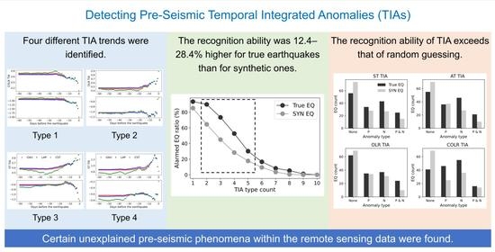
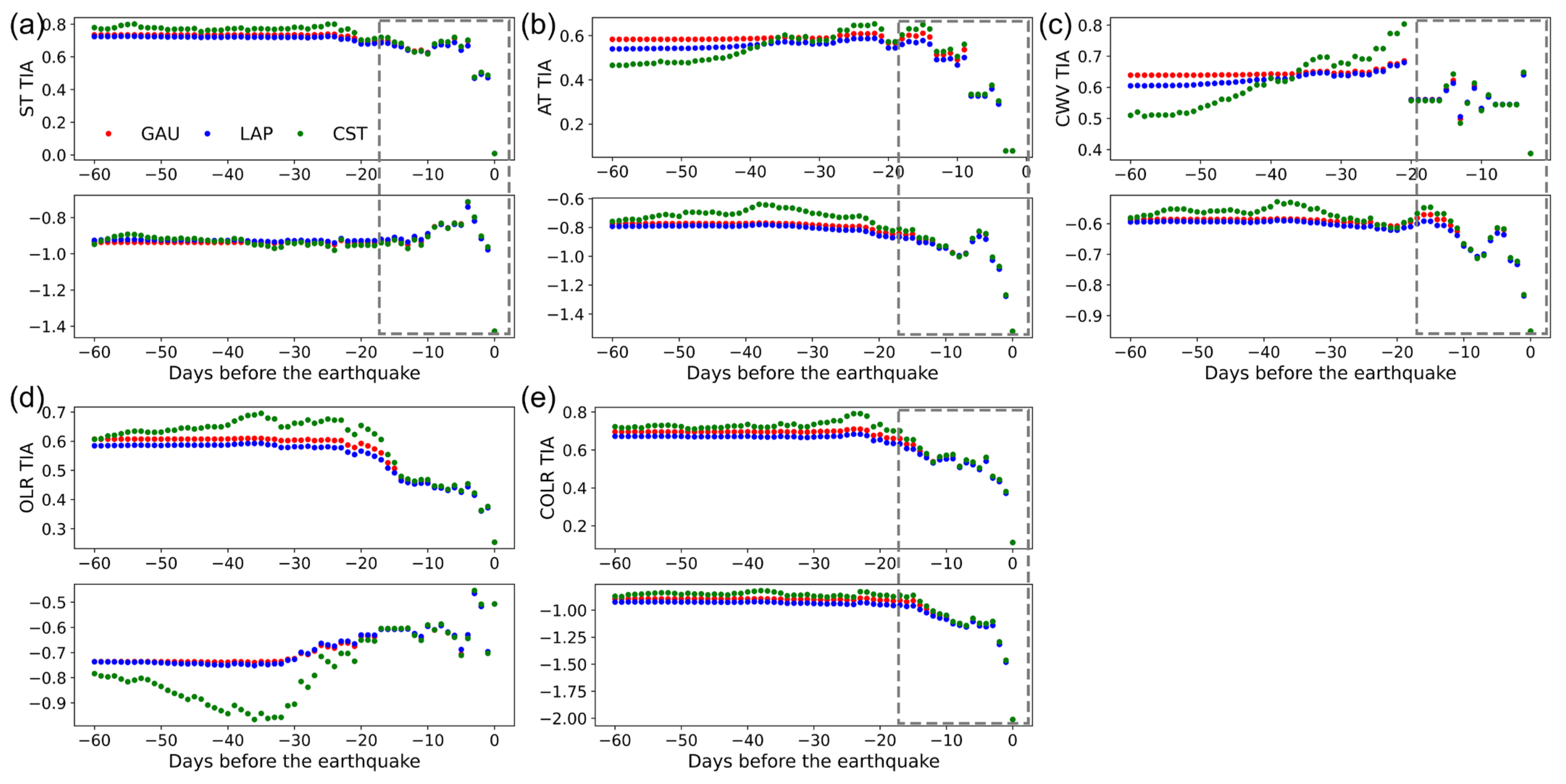
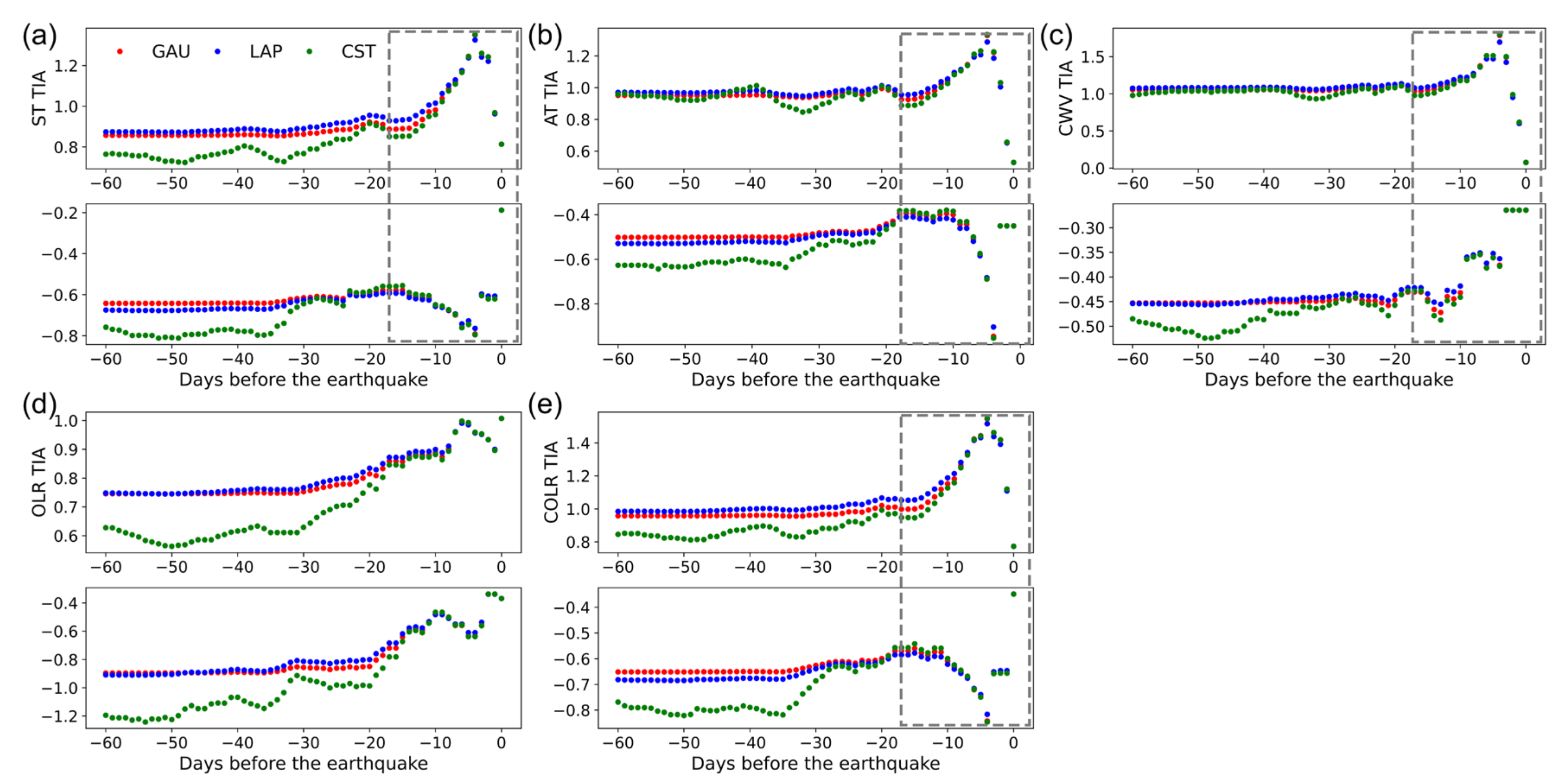
4.1. Trend Characteristics of Multiparametric TIA

The time series of pre-seismic anomalies of different geophysical parameters used in this study was first obtained within 60 days prior to a true or synthetic earthquake. The TIA for each parameter was calculated with different time intervals according to the method described in Section 3.2, and then the calculated TIA values were plotted in a cumulative manner (Figure 3a). For example, the ST TIA value for the 10th day was calculated using data from 0 to 10 days before the earthquake. Thus, the time series indicates the temporal evolution characteristics of pre-seismic anomalies. When anomalies were observed in multiple parameters, a pre-seismic anomaly was identified, and an alarm warned that an M ≥ 7 earthquake would likely take place within the 5° × 5° grid within the next few days (Table 1). We identified four different TIA trends, especially for the first ~30 days prior to the events. For one earthquake, five parameters could present different TIA trends, even when some parameters had no anomalous variation.
Type 1: PTIA and NTIA decrease rapidly before the earthquake with negative anomalies dominating the area near the epicenter (e.g., significant temperature reduction effects) (see ST, AT, CWV, and COLR TIAs in Figure 3). Prior to the 2011 M9.1 Great Tohoku Earthquake, significant crust uplift was detected along with the full southward alignment of Global Positioning System (GPS) azimuths [19], which may have led to cold water upwelling from the seafloor. Meanwhile, in a well 155 km northwest of the epicenter, anomalous decreases in groundwater level and temperature were observed starting 3 months before the earthquake due to possible pre-seismic crustal deformation [44]. These observations could explain negative anomaly phenomena. Similar phenomena can also be observed for inland earthquakes. Significant cooling phenomena along the Himalayas prior to the 2015 Mw 7.9 Nepal earthquake have been reported, and stress relaxation is suggested as a possible explanation [24].
Type 2: PTIA and NTIA increase rapidly before the earthquake with positive anomalies dominating the area near the epicenter (e.g., significant warming effects) (see AT, CWV, OLR, and COLR TIAs in Figure 4). This phenomenon has been reported by many studies; that is, anomalous increases in diverse parameters prior to earthquakes [15].
Type 3: PTIA increases and NTIA decreases rapidly before the earthquake, with both positive and negative anomalies apparent in the area near the epicenter before the earthquake (see ST, AT, OLR, and COLR TIAs in Figure 5). This bidirectional trend indicates strongly anomalous perturbation around the epicenter [45].
Type 4: Similar to Type 3, with either PTIA or NTIA reaching a peak and then rapidly disappearing within several days following the strong earthquakes (Figure 6). This delayed phenomenon was observed for only a small percentage of the tested earthquakes.

4.2. Comparison between True and Synthetic Earthquake TIAs

A higher rate of earthquake alarms was triggered for true earthquakes compared with synthetic earthquakes, and the rates decreased from 93.5% to 0% and from 85.2% to 0% as the number of TIA parameters increased for true and synthetic earthquakes, respectively (Figure 7a). The optimal number of parameters was found to be 2–5, for which the recognition ability for true earthquakes was 12.4–28.4% higher than that for synthetic earthquakes; when >6 TIA parameters were used, the rate of earthquake recognition dropped significantly for both true and synthetic events. In total, we identified 627 TIA for true earthquakes and 430 TIA for synthetic earthquakes. The different TIA types were similar between the true and synthetic earthquakes (Figure 7b,c). For true earthquakes, the NTIAs of ST, AT, CWV, and COLR had slightly more counts; for the synthetic earthquakes, the PTIAs of AT and CWV, and NTIA of COLR had slightly more counts. This suggests that NTIAs tend to correlate with true earthquakes, while PTIAs correlate with synthetic earthquakes. This is consistent with the results of past studies in which significant negative anomalies were confirmed around epicenters [24,45]. For true earthquakes, positive and negative TIAs of AT and CWV had the highest recognition counts (>15); for synthetic earthquakes, positive and negative TIAs of ST and AT had the highest recognition counts (>20) (Figure 7d,e). The TIA trend characteristics before earthquake occurrence were not unique; however, the data revealed certain unexplained anomalous phenomena.
Positive/negative anomalies could have one of four combinations: (1) neither positive nor negative TIA, (2) only positive TIA, (3) only negative TIA, and (4) both positive and negative TIAs. For each geophysical parameter, the likelihood of identifying pre-seismic anomalies was higher for true earthquakes than for synthetic earthquakes (Figure 8). More specifically, synthetic earthquakes had more no-TIA situations, and the counts of the other three combinations were less than those of the true earthquakes. While we identified a small number of exceptions for the AT and CWV TIAs, these results confirm that TIAs for all parameters can identify pre-seismic anomalous signals to some extent (Figure 7). As such, the proposed approach has good potential for predicting future earthquakes. Remote sensing observations from space-borne platforms contain seismogenic information that is subtle and transient compared with the strong background signals from natural processes and anthropogenic activities. As a result, most precursory parameters also had high missed detection and false alarm rates. Moreover, when the false alarm rate was suppressed, the accuracy rate also decreased [45]. The TIA provides the potential to improve forecast accuracy.

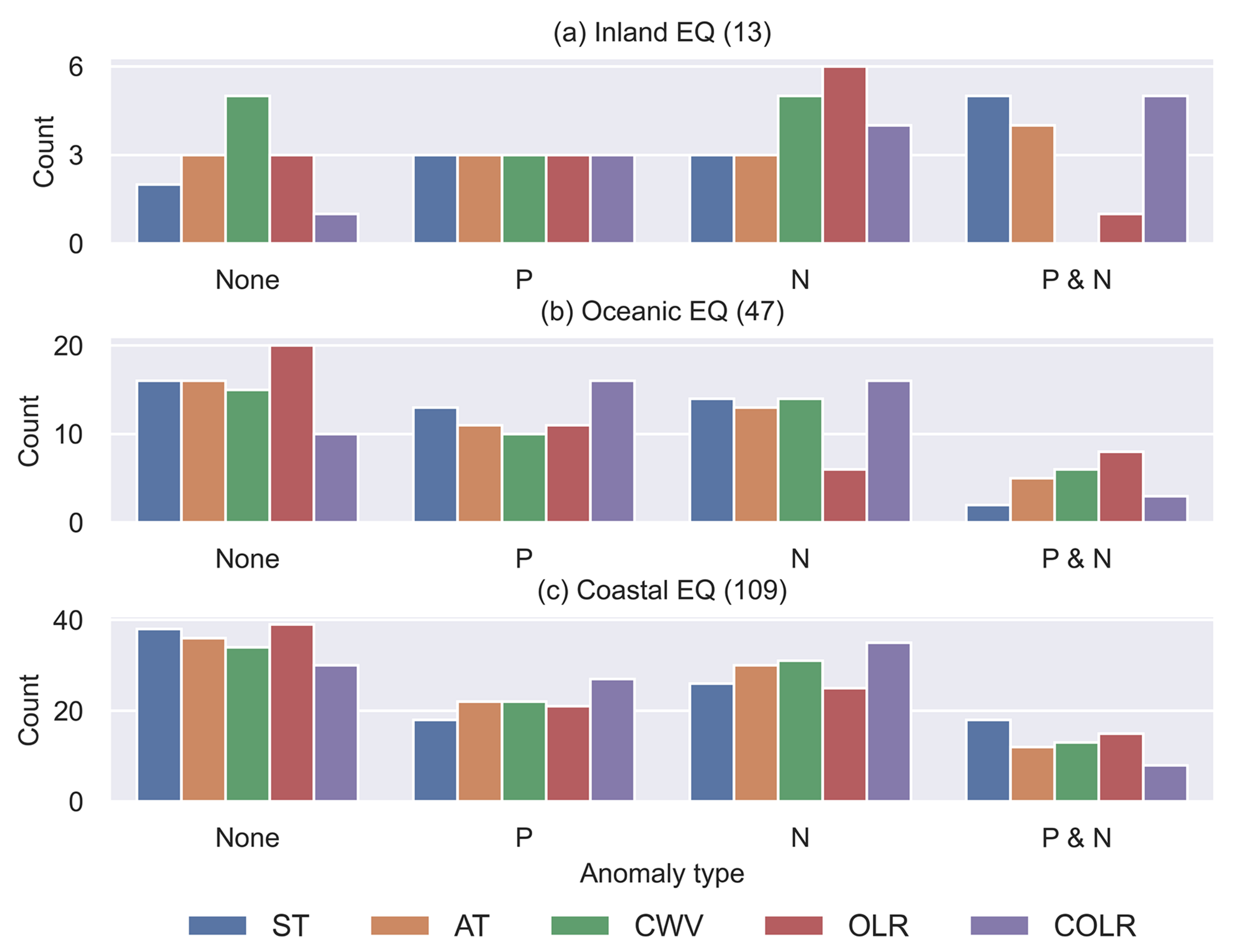
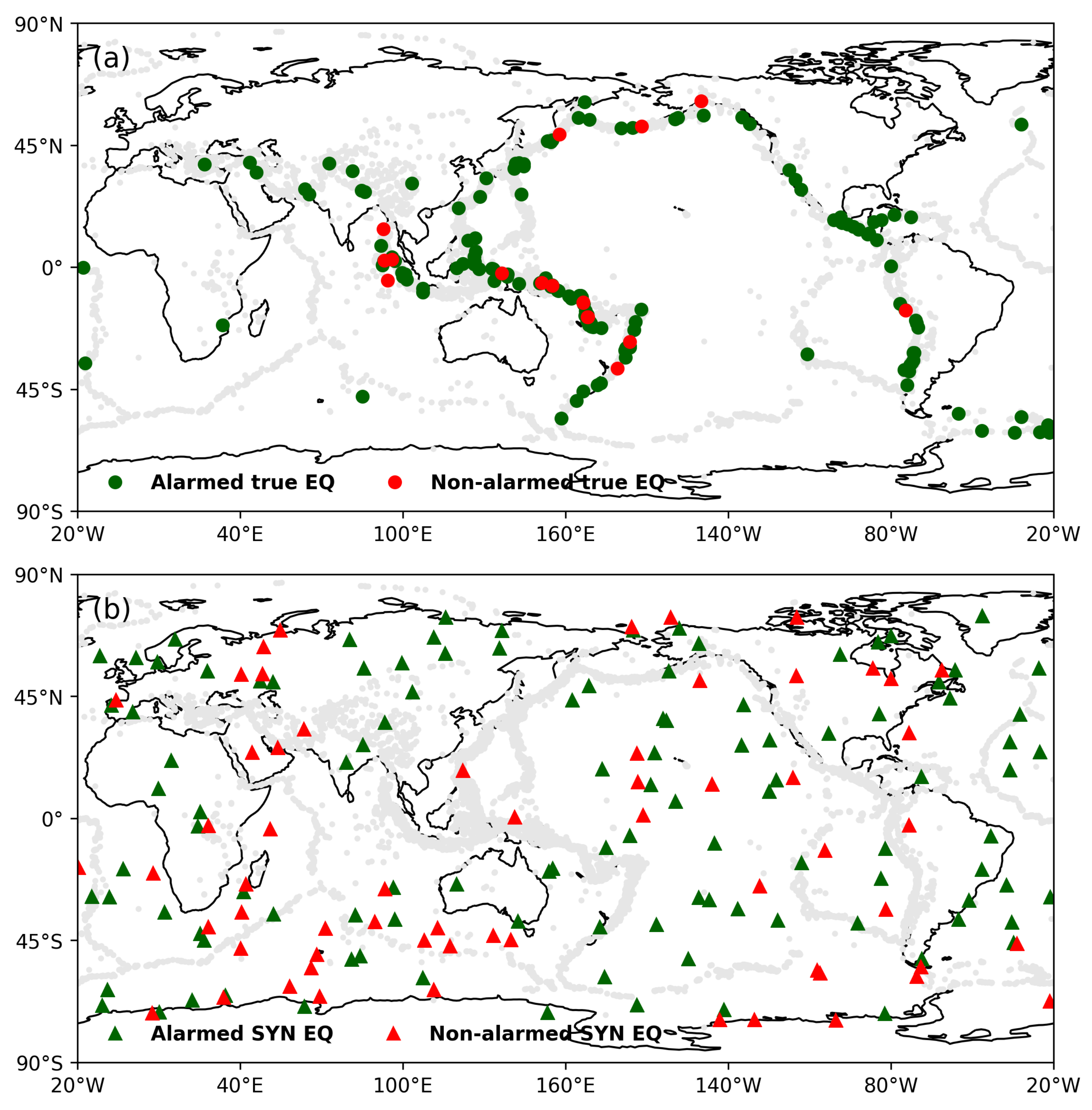
4.3. Statistical Analysis Based on Earthquake Locations

Earthquake location influences anomaly characteristics owing to different underlying surfaces and medium properties. For true earthquakes, coastal earthquakes were the most common (109), and inland earthquakes were the least common (13; Figure 9). OLR and CWV NTIAs recognized more inland earthquakes but with higher missed earthquakes (Figure 9a). COLR TIA had a strong ability to recognize oceanic earthquakes with both positive and negative anomalies. Similar patterns were observed for coastal and oceanic earthquakes (Figure 9c). The synchronous positive and negative TIAs always had poor recognition ability for oceanic and coastal earthquakes. Land cover affects the spatial distributions of diverse parameters, leading to high spatial heterogeneity, while seawater has high thermal inertia, which changes thermal radiative transfer from the seabed to the sea surface [8]. For instance, CWV increased after the 2001 Gujarat earthquake, for which the epicenter was beneath the sea [29]. Significantly reduced sea surface temperatures have been observed prior to some earthquakes and may be related to the upwelling of cold water from the ocean floor [46].
Figure 10 shows the spatial distributions of recognition and non-recognition earthquakes. The recognized rates were higher near earthquake-prone regions (light gray areas). Therefore, the proposed method provides insight into the apparent statistical significance between anomaly phenomena and earthquakes and has a forecasting ability that exceeds that of random guessing. Our results clearly demonstrate that seismically active regions are the most appropriate for testing methods to forecast earthquakes (e.g., in Japan; [32,43]).

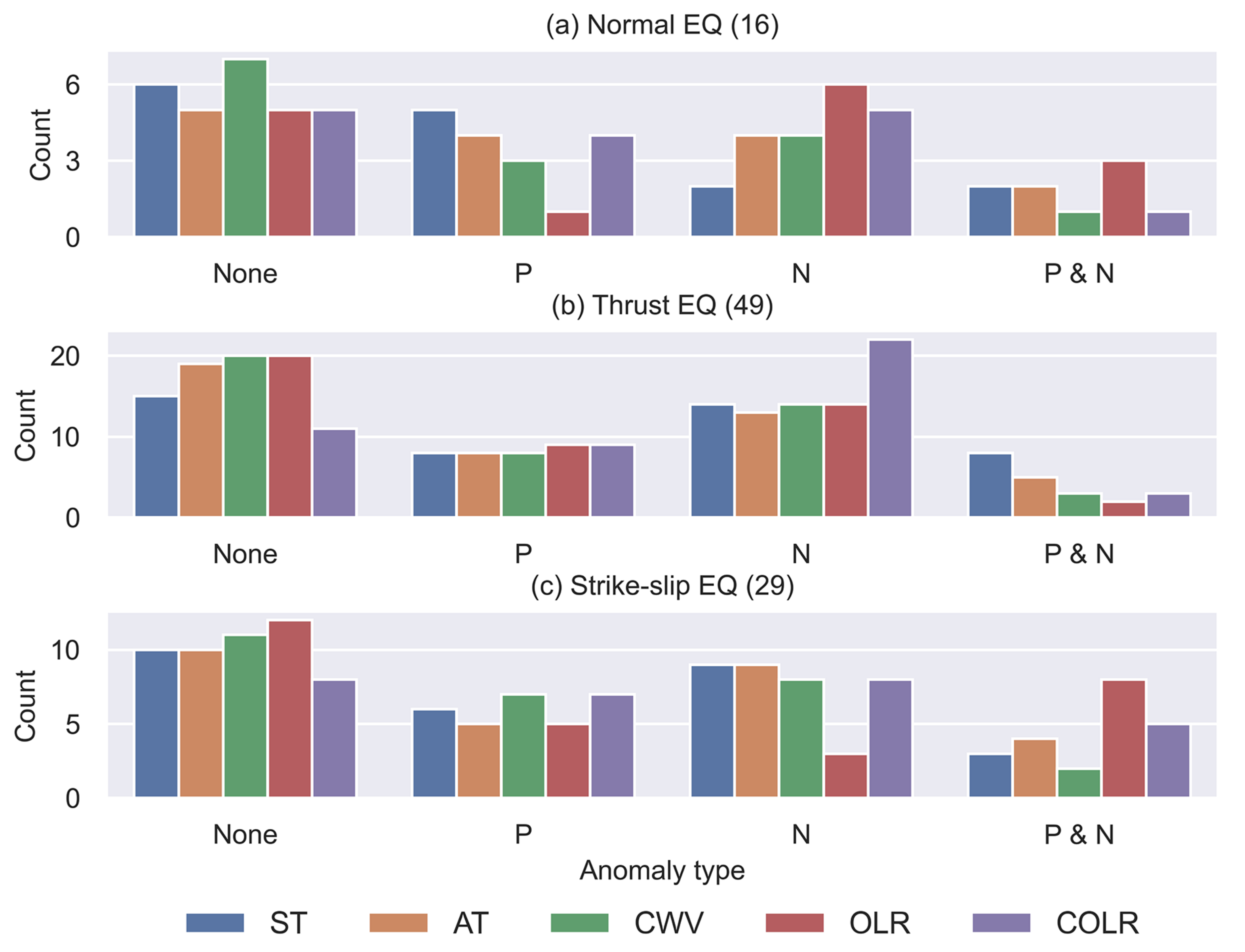
4.4. Statistical Analysis Based on Earthquake Focal Mechanisms

Focal mechanisms were obtained from the GEOFON data center of the GFZ German Research Centre [47]. Focal mechanism solutions, which were only available for 94 of the 169 earthquakes (mostly those after 2011), were classified into strike-slip, normal, and thrust. If more than one type existed for a given earthquake, the major component was chosen. For normal earthquakes in Figure 11a, ST PTIA and OLR/COLR NTIAs showed the best recognition ability. Thrust earthquakes were the most numerous (49 events) and were most commonly associated with NTIAs (Figure 11b). For strike-slip earthquakes, synchronous positive and negative TIAs (particularly OLR/COLR TIAs) had better recognition ability than they did for the other earthquake types. Overall, negative anomalies were the most prevalent phenomena for all earthquake types (Figure 9; [45]).

5. Discussion

5.1. Implications for Earthquake Forecasts

The prediction of earthquakes has been recognized as a global problem [10]. Earthquakes are rapid energy release processes that must produce various anomalous phenomena with respect to normal reference signals [4,19]. The basic assumptions are: (1) the bigger the earthquake, the more obvious the anomalous signals; and (2) the shorter the interval until the earthquake, the clearer the anomalous signals. TIA trend characteristics were observed for both true and synthetic earthquakes; as such, earthquake alarms based on the proposed method come with significant uncertainties. This is a prevalent issue that impedes operational earthquake forecasting. Anomaly detection methods have good performance for retrospective correlation analysis (i.e., high accuracy and low missed detection rates); however, earthquake forecasting based on prospective statistics in seismically active regions has low forecasting capacity [45].
Despite the optimism of some researchers, routine and accurate earthquake forecasting remains a challenge [48]. Therefore, new approaches (e.g., artificial intelligence) need to be developed and verified [21]. The extension of natural time analysis to remote sensing data is also an important aspect, based on the success of this approach, in the detection of precursory phenomena of seismicity, surface displacements, Earth’s magnetic field, and seismic electric signals prior to the strong earthquakes [7,19]. Combining multiple data sources offers the potential to refine the detection of anomalous phenomena [4,15], as confirmed by our results. Therefore, short-term earthquake forecasting models that combine multiple data streams are deemed to be the most promising approach [43]. Moreover, a robust and quantitative evaluation of anomaly detection methods is needed to gain new insights into the feasibility of earthquake forecasts. By constructing a uniform baseline using historical observation data and earthquake catalogs in retrospective and prospective ways [45], we will be better able to compare various approaches and parameters, offering the potential to develop models for integrating precursors and anomaly detection methods for operational earthquake forecasting.

5.2. Underlying Geophysical Mechanisms of Pre-Seismic Anomalies

The findings derived from rock experiments offer an experimental basis for relating temperature anomalies to variations in crustal stress fields and tectonic activities from remote sensing observations [49,50,51,52]. Elastic energy continuously accumulates in the rock mass during earthquake preparation. Both theoretical calculations and laboratory measurements indicate that temperature variations are related to the quantity of volume strain measured under elastic stress conditions for solid materials. The thermal elastic coefficient of roughly 1 mK/MPa is proportional to the principal stress [50,53]. When the volume strain increases due to compression, the temperature also rises, while it will decline in the tensile state. Accompanying thermal effects caused by the change in the strain levels of the deformation field are likely associated with surface temperature, which can be retrieved from thermal infrared (TIR) measurements [54]. TIR radiation field (e.g., ST, AT, and OLR) derived from satellite observations serves as a feasible physical parameter related to regional overall stress fields to some extent in this research field [55].
Fault deformation is always local and mostly deep below the ground surface. However, multiparametric anomalies are widespread and regional at the seismogenic zones. The geophysical mechanism of how the heating derived from fault deformation transfers to the ground surface or the atmosphere is a key point. The thermal conductivity, thermal inertia, and time constant of the thermal diffusion of rocks are the controlling factors for transmitting the Joule temperature to the TIR radiation field. The low heat conductivity of rocks delays the transfer of increased temperatures caused by fault deformation at the scales of months to years, even decades. This is inconsistent with the satellite observation. In p-hole theory [56,57,58,59,60], however, mechanical stresses between rocks lead to the activation of peroxy defects deep in the Earth’s crust. These peroxy defects release electronic charge carriers, electrons e’ and holes h. The h have the remarkable ability to flow out into and through the surrounding rocks that are less stressed or unstressed and to propagate rapidly to the distant regions. When the h arrive on the Earth’s surface, they lead to a series of follow-up reactions. The exothermal recombination of h on the Earth’s surface leads to a stimulated TIR emission, another source of thermal radiation other than Joule temperature, which could be received by satellite sensors.
This work illustrates the extensive TIR measurements that can be derived from a satellite platform. It is worth noting that multiparametric anomalies may reflect the fault activities of tectonically active regions that do not always correspond to an impending earthquake, as the anomaly is not a sufficient condition. Various non-seismic factors affect TIR radiation changes and anomalous features [8], and the triggering of an earthquake is also influenced by intricate geologic conditions, tectonic movements, and dynamic processes.

6. Conclusions

The short-term (days or weeks) pre-seismic period is a critical phase during which stress accumulation becomes stronger and corresponding precursory responses (e.g., ST) likely increase in amplitude. We developed a TIA method to obtain the temporal trend of multiparametric anomalies derived from AIRS products before earthquakes; four types of TIA trends were identified. A total of 169 global earthquakes with magnitudes of ≥7.0 were used to test this new method in a retrospective manner. In addition, we generated 169 synthetic earthquakes to test the suppression capacity of anomaly detection in tectonically non-active areas. A time series-based anomaly removal method was developed to generate the reference fields of ZS methods. Long-term correlation analyses showed that recognition ability was 12.4–28.4% higher for true earthquakes than for synthetic earthquakes (i.e., higher than that of a random guess). TIA incorporating 2–5 parameters was optimal for recognizing the earthquakes, indicating that multiparametric anomalies can provide complementary information to improve statistical significance. Our results confirm the appearance of TIA in spatiotemporal correspondence with forthcoming earthquakes, and some unexplained anomalous signals around epicentral areas were observed. A greater understanding of geophysical mechanisms and the development of new anomaly detection methods would strengthen the uniqueness of pre-seismic anomalous phenomena.

Author Contributions

Conceptualization, Z.J.; methodology, Z.J.; writing—original draft preparation, Z.J.; writing—review and editing, Z.J. and X.S. All authors have read and agreed to the published version of the manuscript.

Funding

This research was funded by the National Key Research and Development Program of China, grant number 2019YFC1509202; National Nonprofit Fundamental Research Grant of Institute of Geology, China Earthquake Administration, grant number IGCEA2002; the China Seismic Experimental Site Project, grant number 2018CSES0205; and the Scientific Research Project of the Shanghai Science and Technology Commission, grant number 14231202600.

Data Availability Statement

AIRS AIRS3STD data are available from the GES DISC at https://disc.gsfc.nasa.gov/datasets/AIRS3STD_7.0/summary (accessed on 10 April 2022). Earthquake catalog data are available from the USGS at https://www.usgs.gov/natural-hazards/earthquake-hazards (accessed on 10 April 2022). Seismic data were obtained from the GEOFON data centre of the GFZ German Research Centre for Geosciences at https://geofon.gfz-potsdam.de (accessed on 10 April 2022).

Conflicts of Interest

The authors declare no conflict of interest.

References

  1. Geller, R.J. Earthquake prediction: A critical review. Geophys. J. Int. 1997, 131, 425–450. [Google Scholar] [CrossRef] [Green Version]
  2. Uyeda, S.; Nagao, T.; Kamogawa, M. Short-term earthquake prediction: Current status of seismo-electromagnetics. Tectonophysics 2009, 470, 205–213. [Google Scholar] [CrossRef]
  3. Bormann, P. From Earthquake Prediction Research to Time-Variable Seismic Hazard Assessment Applications. Pure Appl. Geophys. 2010, 168, 329–366. [Google Scholar] [CrossRef]
  4. De Santis, A.; De Franceschi, G.; Spogli, L.; Perrone, L.; Alfonsi, L.; Qamili, E.; Cianchini, G.; Di Giovambattista, R.; Salvi, S.; Filippi, E.; et al. Geospace perturbations induced by the Earth: The state of the art and future trends. Phys. Chem. Earth Parts A/B/C 2015, 85–86, 17–33. [Google Scholar] [CrossRef] [Green Version]
  5. Uyeda, S.; Kamogawa, M. The Prediction of Two Large Earthquakes in Greece. Eos Trans. Am. Geophys. Union 2008, 89, 363. [Google Scholar] [CrossRef]
  6. Huang, Q. Seismicity Pattern Changes Prior to the 2008 Ms7.3 Yutian Earthquake. Entropy 2019, 21, 118. [Google Scholar] [CrossRef] [Green Version]
  7. Varotsos, P.A.; Sarlis, N.V.; Skordas, E.S. Self-organized criticality and earthquake predictability: A long-standing question in the light of natural time analysis. Europhys. Lett. 2020, 132, 29001. [Google Scholar] [CrossRef]
  8. Jiao, Z.-H.; Zhao, J.; Shan, X. Pre-seismic anomalies from optical satellite observations: A review. Nat. Hazards Earth Syst. Sci. 2018, 18, 1013–1036. [Google Scholar] [CrossRef] [Green Version]
  9. Tronin, A.A. Remote sensing and earthquakes: A review. Phys. Chem. Earth Parts A/B/C 2006, 31, 138–142. [Google Scholar] [CrossRef]
  10. Bakun, W.H.; Aagaard, B.; Dost, B.; Ellsworth, W.L.; Hardebeck, J.L.; Harris, R.A.; Ji, C.; Johnston, M.J.; Langbein, J.; Lienkaemper, J.J.; et al. Implications for prediction and hazard assessment from the 2004 Parkfield earthquake. Nature 2005, 437, 969–974. [Google Scholar] [CrossRef] [Green Version]
  11. Pavlidou, E.; van der Meijde, M.; van der Werff, H.; Hecker, C. Time Series Analysis of Land Surface Temperatures in 20 Earthquake Cases Worldwide. Remote Sens. 2018, 11, 61. [Google Scholar] [CrossRef] [Green Version]
  12. Tronin, A.A. Satellite thermal survey—A new tool for the study of seismoactive regions. Int. J. Remote Sens. 1996, 17, 1439–1455. [Google Scholar] [CrossRef]
  13. Saraf, A.K.; Rawat, V.; Banerjee, P.; Choudhury, S.; Panda, S.K.; Dasgupta, S.; Das, J.D. Satellite detection of earthquake thermal infrared precursors in Iran. Nat. Hazards 2008, 47, 119–135. [Google Scholar] [CrossRef]
  14. Bhardwaj, A.; Singh, S.; Sam, L.; Bhardwaj, A.; Martín-Torres, F.J.; Singh, A.; Kumar, R. MODIS-based estimates of strong snow surface temperature anomaly related to high altitude earthquakes of 2015. Remote Sens. Environ. 2017, 188, 1–8. [Google Scholar] [CrossRef]
  15. Cicerone, R.D.; Ebel, J.E.; Britton, J. A systematic compilation of earthquake precursors. Tectonophysics 2009, 476, 371–396. [Google Scholar] [CrossRef]
  16. Sun, K.; Shan, X.; Ouzounov, D.; Shen, X.; Jing, F. Analyzing long wave radiation data associated with the 2015 Nepal earthquakes based on Multi-orbit satellite observations. Chin. J. Geophys. 2017, 60, 3457–3465. [Google Scholar]
  17. Varotsos, P.; Lazaridou, M. Latest aspects of earthquake prediction in Greece based on seismic electric signals. Tectonophysics 1991, 188, 321–347. [Google Scholar] [CrossRef]
  18. Varotsos, P. The Physics of Seismic Electric Signals; TerraPub: Tokyo, Japan, 2005; p. 338. [Google Scholar]
  19. Varotsos, P.A.; Sarlis, N.V.; Skordas, E.S. Phenomena preceding major earthquakes interconnected through a physical model. Ann. Geophys. 2019, 37, 315–324. [Google Scholar] [CrossRef] [Green Version]
  20. Tronin, A.A. Satellite remote sensing in seismology. A review. Remote Sens. 2010, 2, 124–150. [Google Scholar] [CrossRef] [Green Version]
  21. Kato, A.; Ben-Zion, Y. The generation of large earthquakes. Nat. Rev. Earth Environ. 2020, 2, 26–39. [Google Scholar] [CrossRef]
  22. Bhardwaj, A.; Singh, S.; Sam, L.; Joshi, P.K.; Bhardwaj, A.; Martín-Torres, F.J.; Kumar, R. A review on remotely sensed land surface temperature anomaly as an earthquake precursor. Int. J. Appl. Earth Obs. Geoinf. 2017, 63, 158–166. [Google Scholar] [CrossRef]
  23. Sarlis, N.V.; Skordas, E.S.; Christopoulos, S.-R.G.; Varotsos, P.A. Natural Time Analysis: The Area under the Receiver Operating Characteristic Curve of the Order Parameter Fluctuations Minima Preceding Major Earthquakes. Entropy 2020, 22, 583. [Google Scholar] [CrossRef] [PubMed]
  24. Chen, S.; Liu, P.; Feng, T.; Wang, D.; Jiao, Z.; Chen, L.; Xu, Z.; Zhang, G. Exploring Changes in Land Surface Temperature Possibly Associated with Earthquake: Case of the April 2015 Nepal Mw 7.9 Earthquake. Entropy 2020, 22, 377. [Google Scholar] [CrossRef] [Green Version]
  25. Khalili, M.; Alavi Panah, S.K.; Abdollahi Eskandar, S.S. Using Robust Satellite Technique (RST) to determine thermal anomalies before a strong earthquake: A case study of the Saravan earthquake (April 16th, 2013, MW = 7.8, Iran). J. Asian Earth Sci. 2019, 173, 70–78. [Google Scholar] [CrossRef]
  26. Zoran, M. MODIS and NOAA-AVHRR l and surface temperature data detect a thermal anomaly preceding the 11 March 2011 Tohoku earthquake. Int. J. Remote Sens. 2012, 33, 6805–6817. [Google Scholar] [CrossRef]
  27. Mahmood, I. Anomalous variations of air temperature prior to earthquakes. Geocarto Int. 2019, 36, 1396–1408. [Google Scholar] [CrossRef]
  28. Pulinets, S.A.; Dunajecka, M.A. Specific variations of air temperature and relative humidity around the time of Michoacan earthquake M8.1 Sept. 19, 1985 as a possible indicator of interaction between tectonic plates. Tectonophysics 2007, 431, 221–230. [Google Scholar] [CrossRef]
  29. Dey, S.; Sarkar, S.; Singh, R.P. Anomalous changes in column water vapor after Gujarat earthquake. Adv. Space Res. 2004, 33, 274–278. [Google Scholar] [CrossRef]
  30. Piscini, A.; De Santis, A.; Marchetti, D.; Cianchini, G. A Multi-parametric Climatological Approach to Study the 2016 Amatrice–Norcia (Central Italy) Earthquake Preparatory Phase. Pure Appl. Geophys. 2017, 174, 3673–3688. [Google Scholar] [CrossRef]
  31. Mahmood, I.; Iqbal, M.F.; Shahzad, M.I.; Qaiser, S. Investigation of atmospheric anomalies associated with Kashmir and Awaran Earthquakes. J. Atmos. Sol.-Terr. Phys. 2017, 154, 75–85. [Google Scholar] [CrossRef]
  32. Shah, M.; Aibar, A.C.; Tariq, M.A.; Ahmed, J.; Ahmed, A. Possible ionosphere and atmosphere precursory analysis related to Mw > 6.0 earthquakes in Japan. Remote Sens. Environ. 2020, 239, 111620. [Google Scholar] [CrossRef]
  33. Venkatanathan, N.; Yang, Y.-C.; Lyu, J. Observation of abnormal thermal and infrasound signals prior to the earthquakes: A study on Bonin Island earthquake M7.8 (May 30, 2015). Environ. Earth Sci. 2017, 76, 228. [Google Scholar] [CrossRef]
  34. Marchetti, D.; De Santis, A.; Shen, X.; Campuzano, S.A.; Perrone, L.; Piscini, A.; Di Giovambattista, R.; Jin, S.; Ippolito, A.; Cianchini, G.; et al. Possible Lithosphere-Atmosphere-Ionosphere Coupling effects prior to the 2018 Mw = 7.5 Indonesia earthquake from seismic, atmospheric and ionospheric data. J. Asian Earth Sci. 2020, 188, 104097. [Google Scholar] [CrossRef]
  35. McGuire, J.J.; Boettcher, M.S.; Jordan, T.H. Foreshock sequences and short-term earthquake predictability on East Pacific Rise transform faults. Nature 2005, 434, 457–461. [Google Scholar] [CrossRef]
  36. Lippiello, E.; Marzocchi, W.; de Arcangelis, L.; Godano, C. Spatial organization of foreshocks as a tool to forecast large earthquakes. Sci. Rep. 2012, 2, 846. [Google Scholar] [CrossRef] [Green Version]
  37. Derode, B.; Madariaga, R.; Campos, J. Seismic rate variations prior to the 2010 Maule, Chile MW 8.8 giant megathrust earthquake. Sci. Rep. 2021, 11, 2705. [Google Scholar] [CrossRef]
  38. Bouchon, M.; Durand, V.; Marsan, D.; Karabulut, H.; Schmittbuhl, J. The long precursory phase of most large interplate earthquakes. Nat. Geosci. 2013, 6, 299–302. [Google Scholar] [CrossRef]
  39. Susskind, J.; Blaisdell, J.M.; Iredell, L. Improved methodology for surface and atmospheric soundings, error estimates, and quality control procedures: The atmospheric infrared sounder science team version-6 retrieval algorithm. APPRES 2014, 8, 084994. [Google Scholar] [CrossRef]
  40. Zhu, C.; Jiao, Z.-H.; Shan, X.; Zhang, G.; Li, Y. Land Surface Temperature Variation Following the 2017 Mw 7.3 Iran Earthquake. Remote Sens. 2019, 11, 2411. [Google Scholar] [CrossRef] [Green Version]
  41. Zhao, W.; He, J.; Yin, G.; Wen, F.; Wu, H. Spatiotemporal Variability in Land Surface Temperature Over the Mountainous Region Affected by the 2008 Wenchuan Earthquake From 2000 to 2017. J. Geophys. Res. Atmos. 2019, 124, 1975–1991. [Google Scholar] [CrossRef]
  42. Ouzounov, D.; Pulinets, S.; Romanov, A.; Romanov, A.; Tsybulya, K.; Davidenko, D.; Kafatos, M.; Taylor, P. Atmosphere-ionosphere response to the M9 Tohoku earthquake revealed by multi-instrument space-borne and ground observations: Preliminary results. Earthq. Sci. 2011, 24, 557–564. [Google Scholar] [CrossRef] [Green Version]
  43. Genzano, N.; Filizzola, C.; Hattori, K.; Pergola, N.; Tramutoli, V. Statistical Correlation Analysis Between Thermal Infrared Anomalies Observed From MTSATs and Large Earthquakes Occurred in Japan (2005–2015). J. Geophys. Res. Solid Earth 2021, 126, e2020JB020108. [Google Scholar] [CrossRef]
  44. Orihara, Y.; Kamogawa, M.; Nagao, T. Preseismic changes of the level and temperature of confined groundwater related to the 2011 Tohoku Earthquake. Sci. Rep. 2014, 4, 6907. [Google Scholar] [CrossRef] [PubMed] [Green Version]
  45. Jiao, Z.-H.; Shan, X. Statistical framework for the evaluation of earthquake forecasting: A case study based on satellite surface temperature anomalies. J. Asian Earth Sci. 2021, 211, 104710. [Google Scholar] [CrossRef]
  46. Ouzounov, D.; Bryant, N.; Logan, T.; Pulinets, S.; Taylor, P. Satellite thermal IR phenomena associated with some of the major earthquakes in 1999–2003. Phys. Chem. Earth Parts A/B/C 2006, 31, 154–163. [Google Scholar] [CrossRef]
  47. Quinteros, J.; Strollo, A.; Evans, P.L.; Hanka, W.; Heinloo, A.; Hemmleb, S.; Hillmann, L.; Jaeckel, K.-H.; Kind, R.; Saul, J.; et al. The GEOFON Program in 2020. Seismol. Res. Lett. 2021, 92, 1610–1622. [Google Scholar] [CrossRef]
  48. Allen, C.R. Responsibilities in earthquake prediction: To the Seismological Society of America, delivered in Edmonton, Alberta, May 12, 1976. Bull. Seismol. Soc. Am. 1976, 66, 2069–2074. [Google Scholar] [CrossRef]
  49. Huang, J.; Liu, S.; Ni, Q.; Mao, W.; Gao, X. Experimental Study of Extracting Weak Infrared Signals of Rock Induced by Cyclic Loading under the Strong Interference Background. Appl. Sci. 2018, 8, 1458. [Google Scholar] [CrossRef] [Green Version]
  50. Chen, S.; Liu, P.; Guo, Y.; Liu, L.; Ma, J. An experiment on temperature variations in sandstone during biaxial loading. Phys. Chem. Earth Parts A/B/C 2015, 85–86, 3–8. [Google Scholar] [CrossRef]
  51. Ren, Y.; Ma, J.; Liu, P.; Chen, S. Experimental Study of Thermal Field Evolution in the Short-Impending Stage Before Earthquakes. Pure Appl. Geophys. 2017, 175, 2527–2539. [Google Scholar] [CrossRef]
  52. Wu, L.; Liu, S.; Wu, Y.; Wang, C. Precursors for rock fracturing and failure—Part I: IRR image abnormalities. Int. J. Rock Mech. Min. Sci. 2006, 43, 473–482. [Google Scholar] [CrossRef]
  53. Chen, S.; Liu, L.; Liu, P.; Ma, J.; Chen, G. Theoretical and experimental study on relationship between stress-strain and temperature variation. Sci. China Ser. D Earth Sci. 2009, 52, 1825. [Google Scholar] [CrossRef]
  54. Ren, Y.-Q.; Liu, P.-X.; Ma, J.; Chen, S.-Y. An Experimental Study on Evolution of the Thermal Field of En Echelon Faults During the Meta-Instability Stage. Chin. J. Geophys. 2013, 56, 612–622. [Google Scholar]
  55. Ma, J.; Sherman, S.I.; Guo, Y. Identification of meta-instable stress state based on experimental study of evolution of the temperature field during stick-slip instability on a 5° bending fault. Sci. China Earth Sci. 2012, 55, 869–881. [Google Scholar]
  56. Piroddi, L.; Ranieri, G.; Freund, F.; Trogu, A. Geology, tectonics and topography underlined by L’Aquila earthquake TIR precursors. Geophys. J. Int. 2014, 197, 1532–1536. [Google Scholar] [CrossRef]
  57. Freund, F. Pre-earthquake signals: Underlying physical processes. J. Asian Earth Sci. 2011, 41, 383–400. [Google Scholar] [CrossRef]
  58. Freund, F. Toward a unified solid state theory for pre-earthquake signals. Acta Geophys. 2010, 58, 719–766. [Google Scholar] [CrossRef]
  59. Freund, F.; Kulahci, I.G.; Cyr, G.; Ling, J.; Winnick, M.; Tregloan-Reed, J.; Freund, M.M. Air ionization at rock surfaces and pre-earthquake signals. J. Atmos. Sol.-Terr. Phys. 2009, 71, 1824–1834. [Google Scholar] [CrossRef]
  60. Freund, F. Pre-earthquake signals—Part I: Deviatoric stresses turn rocks into a source of electric currents. Nat. Hazards Earth Syst. Sci. 2007, 7, 535–541. [Google Scholar] [CrossRef] [Green Version]
Figure 1. Characteristics of 169 global earthquakes (EQ) and 169 synthetic (SYN) earthquakes with magnitudes ≥7 and focal depths ≤70 km from 2006 to 2020. (a) Spatial distribution of both true and SYN EQs. The gray circles denote global 15,646 earthquakes with magnitudes ≥5.5 and focal depths ≤70 km from 1980 to 2020, representing global active seismic regions. (b) Temporal characteristics of EQ occurrences. (c) Statistics of interoccurrence time of both true and SYN EQs.
Remotesensing 14 02343 g001
Figure 2. Constant (CST), Gaussian (GAU), and Laplace (LAP) weight integration functions used in the temporal integrated anomaly (TIA) calculation within a 60-day interval. In the LAP and GAU functions, μ is set to 0 and σ is 15. The red, blue, and green dots denote GAU, LAP, and CST weight integration functions, respectively.
Remotesensing 14 02343 g002
Figure 3. Trend characteristics for multiparametric temporal integrated anomalies (TIAs) before the 2011 M9.1 Great Tohoku Earthquake, Japan, demonstrating enhanced negative TIAs close to earthquake occurrence. (a) Skin temperature (ST) TIA; (b) air temperature (AT) TIA; (c) total integrated column water vapor burden (CWV) TIA; (d) outgoing longwave radiation (OLR) TIA; (e) clear-sky OLR (COLR) TIA. The two subfigures for each anomaly show the positive and negative TIAs, respectively. Negative days at the abscissa denote the days before the earthquake. The gray dashed frame indicates the TIA trend characteristics. The red, blue, and green dots denote Gaussian (GAU), Laplace (LAP), and Constant (CST) weight integration functions, respectively.
Remotesensing 14 02343 g003
Figure 4. Trend characteristics for multiparametric temporal integrated anomalies (TIAs) before the 2009 M7.7 Papua earthquake, Indonesia, demonstrating enhanced positive TIAs close to earthquake occurrence. (a) Skin temperature (ST) TIA; (b) air temperature (AT) TIA; (c) total integrated column water vapor burden (CWV) TIA; (d) outgoing longwave radiation (OLR) TIA; (e) clear-sky OLR (COLR) TIA. The two subfigures for each anomaly show the positive and negative TIAs, respectively. Negative days at the abscissa denote the days before the earthquake. The gray dashed frame indicates the TIA trend characteristics. The red, blue, and green dots denote Gaussian (GAU), Laplace (LAP), and Constant (CST) weight integration functions, respectively.
Remotesensing 14 02343 g004
Figure 5. Trend characteristics for multiparametric temporal integrated anomalies (TIAs) before the 2013 M7.7 Awaran earthquake, Pakistan, demonstrating simultaneously enhanced positive & negative TIAs close to earthquake occurrence. (a) Skin temperature (ST) TIA; (b) air temperature (AT) TIA; (c) total integrated column water vapor burden (CWV) TIA; (d) outgoing longwave radiation (OLR) TIA; (e) clear-sky OLR (COLR) TIA. The two subfigures for each anomaly show the positive and negative TIAs, respectively. Negative days at the abscissa denote the days before the earthquake. The gray dashed frame indicates the TIA trend characteristics. The red, blue, and green dots denote Gaussian (GAU), Laplace (LAP), and Constant (CST) weight integration functions, respectively.
Remotesensing 14 02343 g005
Figure 6. Trend characteristics for multiparametric temporal integrated anomalies (TIAs) before the 2015 M7.2 Murghob earthquake, Tajikistan, demonstrating enhanced positive/negative TIAs close to earthquake occurrence. (a) Skin temperature (ST) TIA; (b) air temperature (AT) TIA; (c) total integrated column water vapor burden (CWV) TIA; (d) outgoing longwave radiation (OLR) TIA; (e) clear-sky OLR (COLR) TIA. The two subfigures for each anomaly show the positive and negative TIAs, respectively. Negative days at the abscissa denote the days before the earthquake. The gray dashed frame indicates the TIA trend characteristics. The red, blue, and green dots denote Gaussian (GAU), Laplace (LAP), and Constant (CST) weight integration functions, respectively.
Remotesensing 14 02343 g006
Figure 7. Statistical results of multiparametric temporal integrated anomaly (TIA) trends for true and synthetic (SYN) earthquakes (EQ). (a) Alarmed earthquake ratios as a function of TIA type counts for TIAs based on 5 parameters multiplied by 2 types of positive or negative anomalies; anomaly counts of different TIA types for (b) true and (c) synthetic earthquakes; “P”/“N” before the underscore denotes positive or negative TIA (e.g., ST_P is positive skin temperature TIA); earthquake counts of different TIA types for (d) true and (e) synthetic earthquakes.
Remotesensing 14 02343 g007
Figure 8. Statistical results of temporal integrated anomalies (TIAs) for each geophysical parameter. (a) Skin temperature (ST) TIA; (b) air temperature (AT) TIA; (c) total integrated column water vapor burden (CWV) TIA; (d) outgoing longwave radiation (OLR) TIA; (e) clear-sky OLR (COLR) TIA. ‘None’ denotes neither positive nor negative TIA; P denotes only positive TIA; N denotes only negative TIA; and P & N denotes synchronous positive and negative TIAs.
Remotesensing 14 02343 g008
Figure 9. Statistical results of multiparameter temporal integrated anomalies (TIAs) for (a) inland, (b) oceanic, and (c) coastal earthquakes (EQ). ST, skin temperature; AT, air temperature; CWV, total integrated column water vapor burden; OLR, outgoing longwave radiation; COLR, clear-sky OLR.
Remotesensing 14 02343 g009
Figure 10. Map of alarmed (temporal integrated anomaly [TIA] counts 2 ) and not alarmed earthquakes for both (a) true and (b) synthetic (SYN) events.
Remotesensing 14 02343 g010
Figure 11. Statistical results of multiparameter temporal integrated anomalies (TIAs) for (a) normal, (b) thrust, and (c) strike-slip earthquakes (EQ). ST, skin temperature; AT, air temperature; CWV, total integrated column water vapor burden; OLR, outgoing longwave radiation; COLR, clear-sky OLR.
Remotesensing 14 02343 g011
Table 1. Fundamental forecasting parameters of pre-seismic anomalies in retrospective analyses according to the trend characteristics of multiparametric TIA.
ParametersValues
Time range<10 days
Spatial extent5° × 5° around the epicenter (equivalent of a circle with the radius of ~275 km)
Magnitude≥7
Publisher’s Note: MDPI stays neutral with regard to jurisdictional claims in published maps and institutional affiliations.

