1. Introduction
In the past several decades, with the rapid urbanization and industrialization across many regions of the world, atmospheric pollution became increasingly serious and is already a major social problem [
1,
2]. Especially in China, as the largest developing country, the rate of urbanization increased from 17.9% to 54.8% in years between 1978 and 2015 years and continues to increase [
3,
4]. The average Particulate Matter 2.5 (PM
2.5) concentration in cities reached 62 μgm
−3, 60.8 μgm
−3, and 57 μgm
−3 in 2013, 2014, and 2015, respectively. China became the most PM
2.5-polluted area in the world [
5]. PM
2.5 is considered one of the most important pollutants because of its indirect impacts on health, agriculture production, atmospheric visibility, and climate environment [
6,
7]. In 2001–2006, 165 prefectures’ annual PM
2.5 levels had far and away beyond the national atmosphere quality standard of China (NAQSC, annual average < 35 μgm
−3) [
8]. Many studies showed that PM
2.5 is a key atmosphere pollutant threatening public health [
9,
10]. An increase of PM
2.5 concentration by 10 μg/m
3 causes a 0.40% increase in all-course mortality, a 1.43% increase in deaths caused by respiratory failure, and a 0.53% increase in deaths caused by cardiovascular failure [
11]. It is estimated that PM
2.5 pollution caused 1.2 million premature deaths in China in 2010 and nearly 35% of worldwide deaths [
12].
To explore the factors that affect PM
2.5 concentration can help to better analyze the effects of PM
2.5 pollution. A number of literatures showed that human activities and natural factors act on PM
2.5 pollution concentrations either through direct or indirect influences. These influences may be social economy [
2,
13], the industrial structure [
5], climate change [
14], seasonality [
15], or the prevalence of monsoons [
16]. For example, Xu found that economic growth had the large impact on PM
2.5 [
5]. Most studies found a clear reverse “U-shaped” curve between economic development levels, urbanization, and atmosphere pollution, and with improving economy levels, most cities are at a stage of increasing pollution levels [
2,
17]. It was confirmed that PM
2.5 pollution is influenced by seasons and regions, and the highest levels were found in winter despite differences in temperature and relative humidity among different regions. He and his colleague applied the global regression model, and found that increased fossil energy consumption leads to an increase in PM
2.5 concentrations, while elevation, precipitation, temperature, and GDP per capita are all likely to reduce the impact of PM
2.5 pollution [
18].
Moreover, many studies showed that urban planning exert a positive effect on the reduction of PM
2.5 levels over recent years. Examples for these factors are a reasonable urban form, the moderate reduction of road density, building density, population ratios, and improving green spaces [
19]. Of course, there are also studies that used comprehensive indicators in the urbanization process to explore the impact on PM
2.5, for example, the Liveability and Health Index (LHI) [
20]. Urban form, which includes a city area as well as its shape and layout, can be defined as urban land use organization and human activity arrangement [
21], and it is usually measured by several landscape indicators of a city. PM
2.5 pollution is affected by vehicle use, green land, pollutant diffusion, and the heat island effect [
22]. Research proved that higher urban compactness and less fragmentation (i.e., the largest patch index (LPI)) can reduce PM
2.5 pollution in China [
23,
24]. However, other studies argued that motor vehicles are the main cause of atmospheric pollutants emission in cities, and there is a strong correlation between PM
2.5 and mortality in the traffic emission [
25]; thus, a more compact development alone may still increase local PM
2.5 concentrations and also cause more population to be affected by PM
2.5 [
26]. In the USA, controlling the population, the level of urbanization, and the mixing of different land cover types were found to be important influencing factors between pollutant levels and atmospheric quality [
27,
28]. In addition, the distance from the main road, the standard deviation of the building floor, and the average floor are the main urban morphological characteristics that affect the spatial variation of a variety of pollutants [
29]. In the above analysis, because of the complexity of socioeconomic and natural conditions, the relationship between urban form and PM
2.5 may be inconsistent and complex. Scientific urban planning can effectively reduce urban PM
2.5. Therefore, it is necessary to explore the effect of urban form on PM
2.5.
Investigating PM
2.5 concentration is important for research. A large number of experiments used to study the relationship between PM
2.5 and urban form to identify better approaches for reducing atmosphere pollution. Most studies used linear regression models to analyze the urban form indexes that are related to PM
2.5 pollution and estimated the coefficient of form indexes in the model [
30]. In addition, spatial econometric models and the Environmental Kuznets curve (EKC) hypothesis were used to study the socioeconomic and natural factors on urban atmosphere pollution [
13,
31]. Most studies mainly obtained urban form data through urban land use data and calculated the urban landscape pattern index to represent specific characteristics of the urban form. Most models selected class area (CA), number of patches (NP), patch density (PD), LPI, area-weighted mean shape index (AWMSI), percentage of landscape (PLAND), aggregation index (AI), landscape shape index (LSI), contiguity index (CONTIG), effective mesh size (MESH), interspersion juxtaposition index (IJI), and other landscape pattern indexes [
32,
33]. PM
2.5 data are obtained in three main ways: monitoring real-time data through environmental observation sites, monitoring through experimental instruments, and estimating PM
2.5 concentrations using atmospheric aerosol optical depth (AOD) data obtained from remote sensing images [
34]. The latter can compensate for the shortcomings of experimental technology and ground monitoring sites and provides large-scale and real-time continuous observation data [
35]. Although many studies explored the correlation between urban form and PM
2.5 pollution at different scales from different-sized cities to urban agglomerations to countries, more specific urban form indicators need to be analyzed in the case of China. For example, there is a lack of variables explaining the effects of local meteorological conditions on the spatial aggregation and dispersion of PM
2.5 pollution. The geographical conditions of China are complex, and the urban forms of different geographical locations vary greatly; therefore, it is necessary to develop more specific urban form indicators to evaluate the shape of cities from different aspects and to measure the urban forms of China more adequately.
To develop more effective urban development strategies that can alleviate air pollution, as well as integrate the strengths and weaknesses of previous scientific research, this paper assesses the relationship between urban form and PM2.5. For this, multisource data is used to establish an index system of urban form. Estimates of PM2.5 concentrations are based on AOD data. Based on 340 prefecture-level cities in China, the linear regression model is applied to study the correlation between urban form and PM2.5. Next, a geographically weighted regression (GWR) model is used to analyze the geographical differentiation of the impact urban form exerts on pollutant emissions. PM2.5 concentration data and other natural factors are derived from satellite-derived data. Then, a comprehensive evaluation system of urban form indicators was established by using land use data and road network data. Next, the results of the linear regression method and GWR model between urban form and PM2.5 concentration are analyzed. The paper ends with a discussion of the research results and presents relevant policy implications.
3. Results
3.1. Spatial Distribution Characteristics of PM2.5
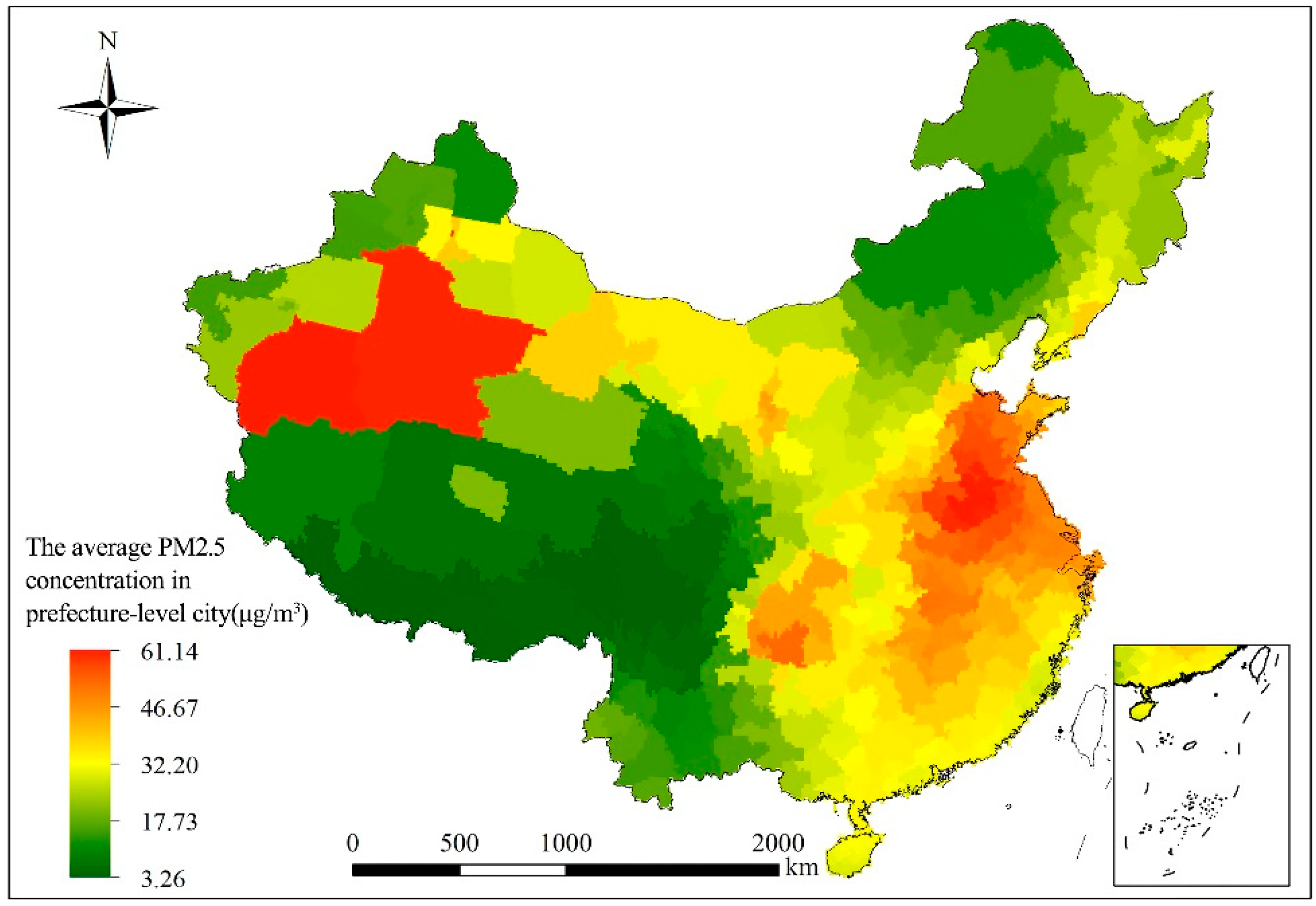
Figure 2 illustrates the geographic distribution of the average PM
2.5 concentrations of China’s cities in 2015, clearly indicating that the spatial distribution of PM
2.5 is heterogeneous. Overall, cities in eastern China tend to have higher PM
2.5 levels than cities in western China, and cities in northern China have higher PM
2.5 levels than cities in southern China. Specifically, areas with highest PM
2.5 levels are concentrated in the North China Plain and Sichuan Basin, as well as in parts of the Northwest China. Among these, the high PM
2.5 level-area of the northwest region is mainly caused by the Taklamakan desert (the world’s second largest desert), where perennial wind and sand influx causes extremely rich suspended particulate matter; therefore, the concentration of PM
2.5 in the desert area is high. The level of economic development in the North China Plains is high. The development of pollution-intensive industries in North China promotes regional economic development, and therefore, man-made atmospheric pollutant emissions are very large. In the southwest region, area with high PM
2.5 pollution is mainly concentrated in the Sichuan Basin, a region that is particularly affected by humidity and precipitation, which causes rich suspended particles in the atmosphere. Moreover, the special structure of the terrain is not conducive to the spread of pollutants, and the population of the region causes high levels of anthropogenic pollution emissions. Because of its elevation, the Qinghai–Tibet Plateau has a thin atmosphere, these conditions are not conducive for the formation and accumulation of particulate matter in the atmosphere. Therefore, the lowest PM
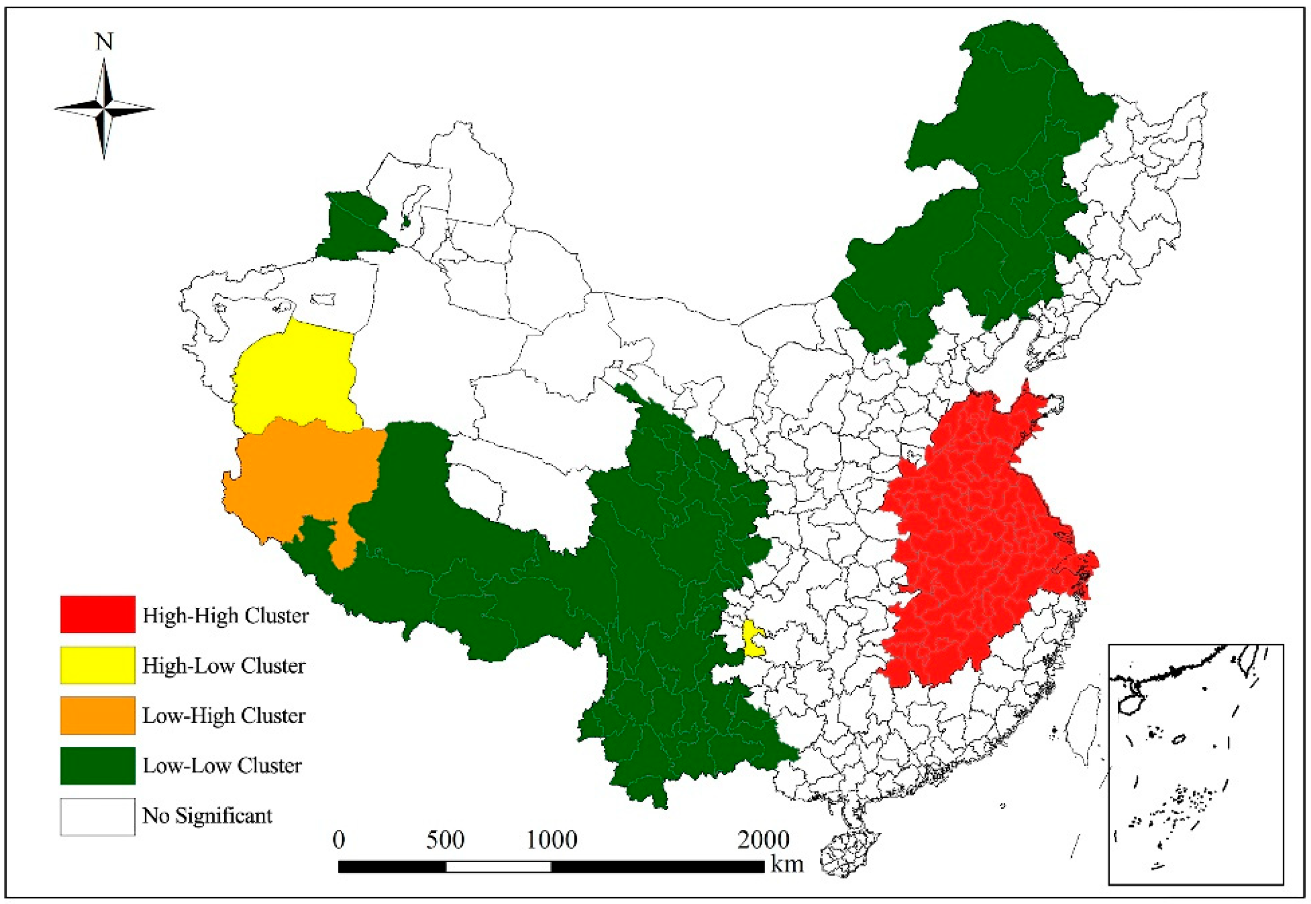
2.5 levels were found in the Qinghai–Tibet Plateau. The global Moran’s I index for PM
2.5 levels were 0.765 (
p < 0.01), indicating a relatively strong positive spatial correlation. Local indicators on PM
2.5 spatial association (LISA) maps show similar typical distributions, with a high PM
2.5 cluster in the North China Plains and a low PM
2.5 cluster in the Northeast China and the Qinghai-Tibet Plateau regions (
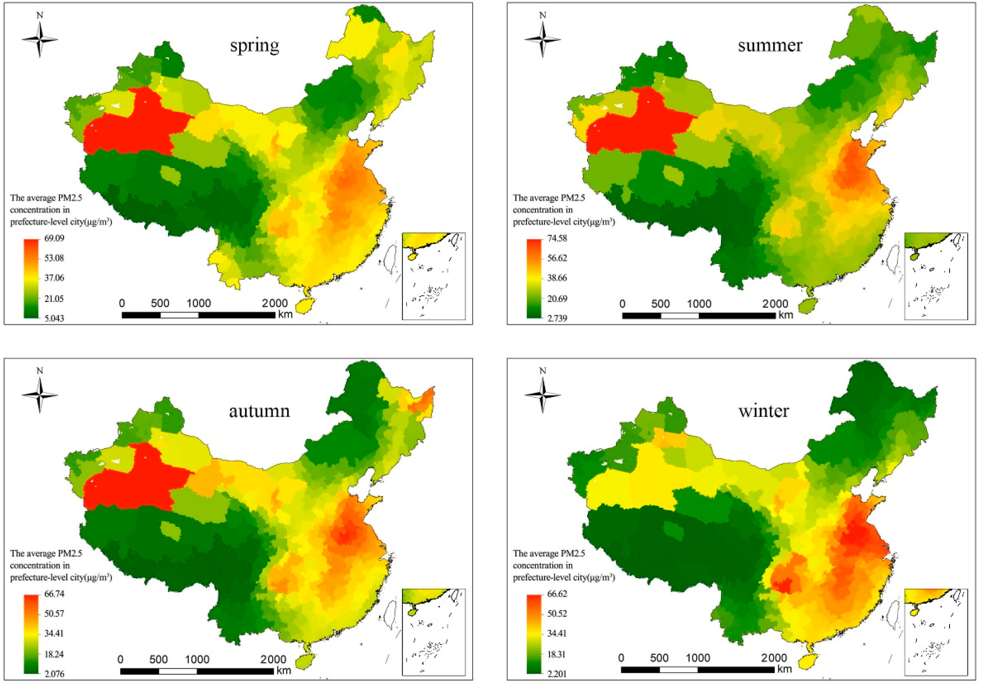
Figure 3). Seasonally, winter had the highest PM
2.5 level, followed by spring, autumn, and summer. However, North China has always been a region with severe PM
2.5 pollution, especially in winter, where the climate is not conducive to the diffusion of atmospheric pollutants [
45]. On a seasonal scale, winter had the highest PM
2.5 level, followed by spring, autumn, and summer. However, North China was always a region with severe PM
2.5 pollution, especially in winter, where the climate is not conducive to the diffusion of atmospheric pollutants. It is worth noting that Southern China always had low PM
2.5 pollution because of its advantageous climate (
Figure 4).
3.2. Correlations between Urban Form and PM2.5
Table 3 shows the results of global regression model analysis (i.e., OLS, SLM, and SEM). The results of suitability statistics such as R
2, AIC, and log-likelihood imply that the spatial analysis technique is more suitable for this data. R
2 values of OLS, SLM, and SEM models are 0.601, 0.943, and 0.874, respectively. These results show that the spatial effect is important in regression analysis and thus, ignoring the spatial effect will reduce the effectiveness of the model. In addition, R
2, AIC, and log-likelihood test results show that the spatial lag effect is more significant.
The results of OLS indicate that most urban form indicators are significantly correlated with PM2.5 concentrations, and six urban form indicators showed significantly (p < 0.01) positive relationships with city-level annual mean PM2.5 levels. Among these six significant factors, LPI, PLAND, and LSI also have a significant impact. LPI has a significant negative correlation with PM2.5 levels, indicating that a better continuity of the urban form leads to a lower fragmentation, and a better atmospheric quality. PLAND and LSI were significantly positively correlated with PM2.5 levels, indicating that the more complex the urban form, the worse the atmospheric quality. AI indicators on PM2.5 concentration is not significant. The four landscape pattern indicators indicate that the fragmentation and complexity of the urban form exert a significant impact on PM2.5 levels, and thus, more attention should be focused on urban form area expansion and the internal composition of fragmentation and complexity. RD is negatively correlated with PM2.5 levels, and the higher the density of the road network, the lower the atmospheric pollution levels. In addition, there is a significant negative correlation between temperature and precipitation and PM2.5 pollution, which confirms that meteorological conditions are conducive to the spread and reduction of atmospheric pollutants. Among other control indicators, SIP has a significantly positive impact on PM2.5 pollution, and PD and PRGDP are positively correlated with PM2.5 levels. Therefore, the development of the secondary industry has a more significant impact on atmospheric pollution.
The SLM model has the best regression results, indicating that urban form and atmospheric pollution have clear spatial dependence. Among the major urban form indicators, LPI was significantly negatively correlated with PM2.5 levels, AI, PLAND, and LSI were significantly positively correlated with PM2.5 pollution, and RD was negatively correlated with PM2.5 levels. In addition, the correlation between temperature and precipitation on PM2.5 was significant (the more precipitation, the lower the temperature), which is beneficial for reducing PM2.5 concentrations in the atmosphere. This is consistent with literature. Therefore, clear spatial correlation exists between urban form indicators and PM2.5 levels. the analysis process of the global regression model analysis has limitations. The GWR model can be used for further analysis by adding the relationship of spatial location.
3.3. Spatial Features of Urban Form on PM2.5
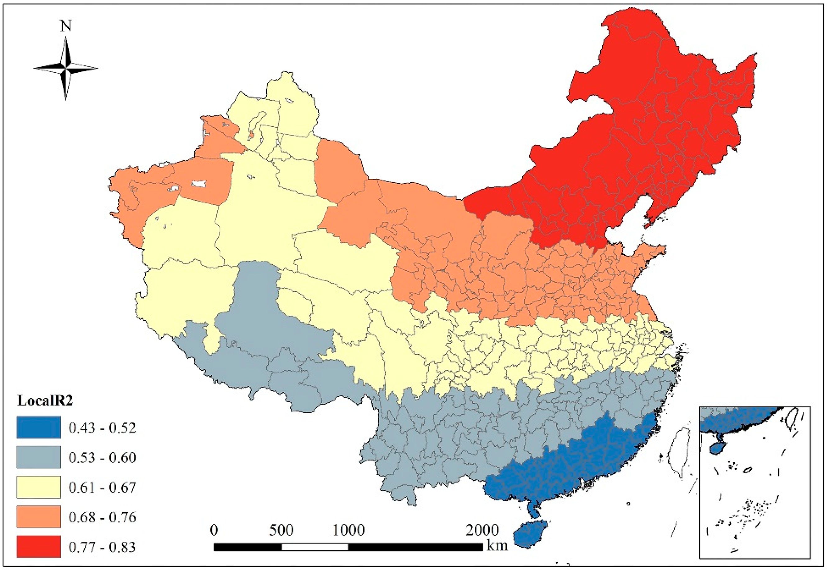
The coefficient of determination of the GWR model was 0.77, and the results of AIC and variance analysis (F test) showed that the results of the model are statistically significant. All 10 variables show noncollinearity and are used under the AIC minimization standard. The GWR model is superior to the OLS model.
Figure 5 shows a distribution map of the regression fitting coefficient R
2 in the regression results for prefecture-level cities. The spatial distribution of R
2 shows that the fitting results of the 10 variables of the urban form range between 0.43 and 0.83, indicating that the 10 indicators selected in this paper exert a stronger comprehensive impact on urban PM
2.5 levels. Moreover, the R
2 value in the spatial distribution decreases from north to south. Therefore, the urban form system has a stronger explanatory power for the urban form of the northern region. On the one hand, this paper uses temperature and precipitation as control variables of two natural factors. They exert a significant positive effect on reducing atmospheric pollutants. The role of climatic factors is more significant in the south, thus reducing the concentration of urban PM
2.5 pollution. On the other hand, this may be due to a lack of estimation of nitrate levels in the PM
2.5 data used in this paper, and therefore, the impact of using a large amount of coal for heating in winter in northern regions may be underestimated, resulting in a low degree of fitting for northern regions. The further south a city is located, the more the explanatory power for PM
2.5 of the urban form decreases.
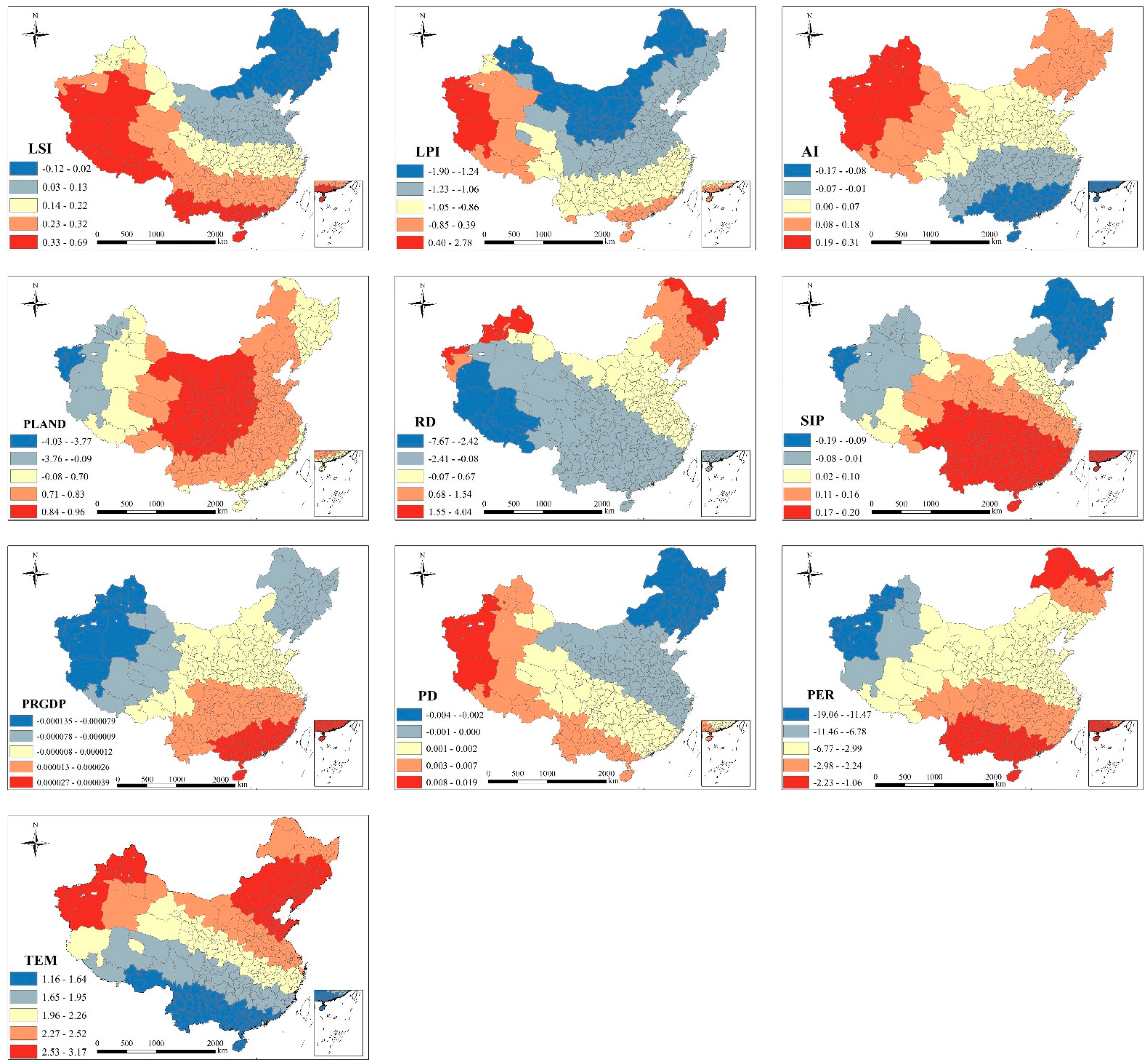
In the GWR model, each urban form index has a specific regression coefficient for the influence degree of PM
2.5 levels, and each coefficient has a different spatial distribution law (
Figure 6). The spatial distribution can more intuitively depict the influencing effect and changing trend between different urban form indicators and cities. In addition, different indicators exert different positive and negative impacts on PM
2.5 levels, and their proportions differ. This also indicates that the influence index is not spatially stable and shows spatial heterogeneity (
Figure 5). The directions of significant relationships were not the same for the studied cities, even for the same factor.
The regression coefficient of urban form index decreases in the order of RD, PLAND, LPI, LSI, and AI. The correlation between road density and PM2.5 levels is highest. Construction dust from the construction phase of roads is the main cause of PM2.5 pollution, followed by pollution caused by motor vehicle driving, as well as more harmful gases that are discharged during traffic congestions. The regression coefficient ranges from 7.7 to 4.0 and decreases from northeast to southwest. In China’s major urban areas, the density of road networks is negatively correlated with PM2.5 concentrations. Improvement of the road network system can effectively reduce traffic congestions and atmospheric pollution. The correlation coefficient between PLAND and PM2.5 concentrations is high and negative. This coefficient mainly measures the size of the area occupied by urban construction land in the whole urban landscape. The influencing factor follows a decreasing trend from center to surrounding areas. Cities where construction land is the main land use type are more likely to cause atmospheric pollution. Developed areas in the south are less affected but may be affected by increasing levels of urban construction, where the application of scientific dust reduction measures and the use of green materials are conducive for reducing emissions of atmospheric pollutants such as building dust. Cities in part of the central and western regions are more susceptible to the impact of the area of construction land. Therefore, reasonable increases of urban construction area and improvement of the level of building construction technology (e.g., green building materials and dust reduction) can reduce PM2.5 concentrations to a certain extent. LPI exerts a significant influence on urban PM2.5 concentrations, where a continuous increase of LPI indicates that the landscape dominance of urban construction land increases, the degree of spatial connection increases, and the intensity of human activities also increases. The values range from −1.9 to 2.8 and increase from north to south with the continuous development of urban construction, which causes more atmospheric pollution. In southern China, driven by the reform and opening up policy, the urbanization level grows faster, and human activities are more intense. This indicates that enhancing the connectivity and dominance of urban construction land has a significant impact on reducing PM2.5 concentrations. A higher LSI index indicates stronger fragmentation and more complicated urban areas. Most regression coefficients between LSI and PM2.5 concentrations are positive, with values ranging from −0.12 to 0.69, indicating that a higher LSI value represents higher levels of PM2.5 pollution. The spatial increase from north to south may be due to the complexity and fragmentation of the shape of the landscape of urban construction land, which leads to an increase of people’s daily commuting time and distance, thus also increasing the pollution caused by the heavy use of commuting means. The impact degree of the southern region is large, indicating that the complexity of urban landscape in the southern region is more likely to affect the PM2.5 levels. AI is used to measure the agglomeration and compactness of urban construction land. The regression coefficient ranges from −0.17 to 0.31, and it changes from negative to positive from north to south. The higher the compactness of urban construction land, the lower the PM2.5 concentrations. Compact urban construction can shorten people’s travel distance, improve the efficiency of land use, and reduce energy consumption. Therefore, in the process of urban development, compact and continuous urban construction is conducive to the improvement of urban atmospheric quality.
Among control indicators, the influences of the three socioeconomic factors on urban PM2.5 pollution show clear spatial differences. In most urban areas, SIP has a significant positive effect on PM2.5 concentrations, indicating that industrial activities aggravate the PM2.5 concentrations in Chinese cities, which is consistent with the literature. The effect of SIP on PM2.5 concentrations in southern China is strong, indicating that reducing the proportion of output of the secondary industry in southern China can significantly improve atmospheric quality. At the same time, the population density in the southeast coastal areas exerts a greater impact on the PM2.5 concentrations. Economic development prompted the migration of many people to the south to work or live. The increased population density has caused more man-made atmospheric pollutant emissions, which strongly impact atmospheric pollution. The overall coefficient of PCGDP is low and its influence is weak. However, in the process of urban development, the improvement of the economic level exerts a significant positive effect on reducing PM2.5 pollution levels.
Reasonable increases in the area of urban construction land and improvements of the level of construction, reducing the fragmentation of urban construction land, compacting urban construction, improving traffic accessibility, applying a reasonable road network density are all very beneficial factors for the improvement of urban atmospheric quality. These can, to a certain extent, reduce the concentration of PM2.5. However, as urbanization continues to increase, the different geographical location, scale and level of construction, and development of the city should be considered according to local conditions, thus providing planning and construction guidance. Urban form can affect PM2.5 concentrations from different aspects. Urban area, geographical location, and economic development level have an impact, and thus also need further discussion and analysis in the future.
4. Discussion
On an annual scale, urban planning factors (e.g., the area of urban construction land, construction fragmentation, and road network density) all exert a specific influence on PM
2.5 levels. At the same time, the economic development of a city is also closely related to PM
2.5 levels. China’s rapid urbanization led to structural changes of its economy, and large areas of land are being used by energy-intensive and labor-intensive industries. In addition, many people move from rural areas to cities, where the population grows rapidly, which increases the release of large amounts of man-made atmospheric pollutants emission. The study showed that temperature and precipitation (as control variables) were significantly correlated with PM
2.5 concentrations in 340 cities in China, and climatic factors played a significant role for reducing atmosphere pollution. Therefore, we further discussed this paper discusses the relationship between urban form and PM
2.5 in different seasons. Seasonality can affect atmospheric quality through changes in precipitation, wind, relative humidity, monsoons, and other diffusion conditions [
16,
30]. When seasonal variations are considered, different seasons exert different impacts on PM
2.5 through different urban form indicators. The SLM model achieved the best regression results, and the relationship between urban form and PM
2.5 in different seasons is discussed through this model (
Table 4).
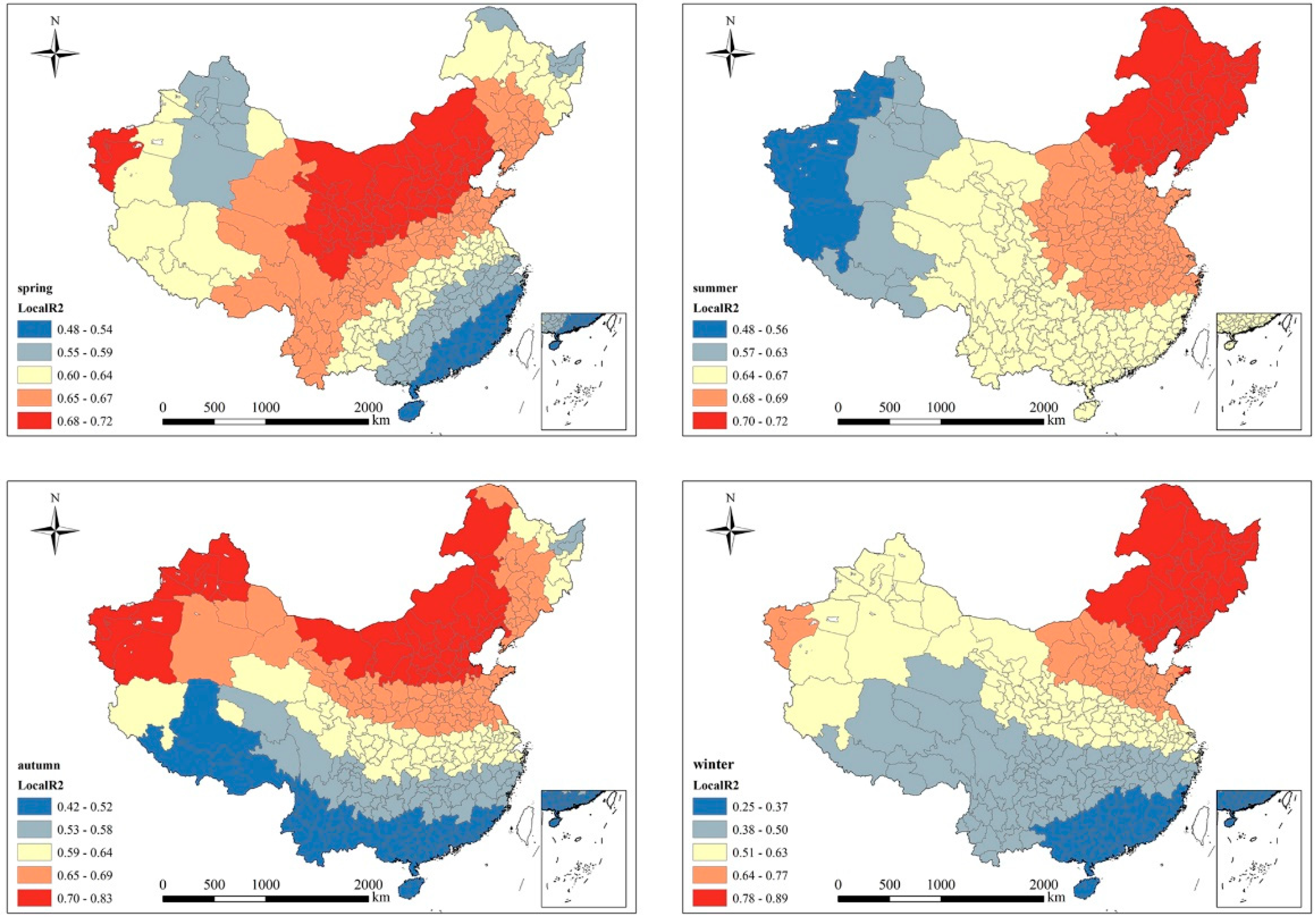
Table 4 shows the results of the regression model, in which the R
2, log-likelihood, AIC, and other statistical results are significantly higher, indicating that the SLM regression model in this study has a relatively good fit. This model can accurately assess the impact of seasonal changes in the urban form on PM
2.5 concentrations. In addition, the seasonal analysis according to the GWR model shows that the regression coefficients of the impact of each city’s form index on the level of PM
2.5 pollution have different spatial distribution patterns (
Figure 7). As shown in
Table 4, seasonal variation significantly affects the relationship between urban form and PM
2.5 concentration.
The four main findings of this study are summarized in the following: firstly, a significant correlation exists between urban form and PM2.5 concentrations in all four seasons, with the highest R2 value in winter. Secondly, the temperature and precipitation in the control variables always exerted a significant impact on PM2.5 concentrations, while other socioeconomic indicators had no significant impact on PM2.5 concentrations. Thirdly, the effect of PLAND and PM2.5 concentrations is significantly positively correlated, while that of LPI and PM2.5 concentrations is significantly negatively correlated in spring, summer, and winter. Fourthly, a negative correlation was found between the density of urban road network and PM2.5 concentrations. Specifically, in spring, LPI, PLAND, and RD significantly impact PM2.5 concentrations, with regression coefficients of −0.289, 0.243, and −1.537, respectively. In the summer, urban compactness (AI = 0.052) can decrease the PM2.5 concentration to some extent. LPI (−0.489) and PLAND (0.320) were all significantly associated with PM2.5 concentrations. In the autumn, the correlation between urban form and PM2.5 concentrations was not significant. In the winter, PLAND (0.240) was significantly positively correlated with the PM2.5 concentrations. LPI (−0.258) and RD (−1.728) were significantly negatively correlated with PM2.5 concentrations.
Therefore, data analysis showed that seasonal change exerts a certain influence on the relationship between urban form indicators and PM
2.5 concentrations. Especially in spring and winter, increasing the connectivity of urban construction land and improving the efficiency of land use within a city can effectively decrease urban PM
2.5 concentrations [
15]. Moreover, increasing the road connectivity also exerts a significant effect on reducing atmosphere pollution. However, the season of autumn does not exert a significant effect on the relationship between urban form and PM
2.5 concentrations. In contrast, the indicators between urban form and PM
2.5 are more significantly correlated in spring and winter, and relatively less in summer and autumn. Firstly, the previous analysis on an annual scale shows that the compact and continuous urban construction land, the reduction of urban land fragmentation, and the reasonable road network density are all conducive to reducing urban atmospheric pollutant emissions. Secondly, seasonal changes are mainly reflected by different climatic variables. The strong Asian monsoon during summer and the subtropical high during autumn result in favorable weather conditions that clean the air from atmospheric pollutants, as they enhance the mobility of the atmosphere above urban centers. The summer monsoon climate moves more precipitation to North China, and at the same time increases the wind speed under the subtropical high pressure. These meteorological conditions are conducive to reducing atmosphere pollutants [
16]. Under such climatic conditions, small changes in the structure of building areas or land areas near the ground exert little impact on atmospheric pollutants. Finally, low temperatures in winter and spring cause the atmospheric flow to sink and wind speeds are also lower than in summer [
15]. In addition, more coal is burnt in the north in winter, and the resulting atmospheric pollutants cannot easily spread and remain concentrated near the ground. Under these conditions, the irregular urban form near the ground has a more significant impact on PM
2.5 concentrations. Therefore, seasonal changes exert a significant impact on PM
2.5 concentrations. When exploring the relationship between urban form and PM
2.5 concentrations, focusing on the results of spring and winter is more effective.
There are many factors that affect the PM
2.5 concentration, but our research just focused on the urban form. In addition, industrial areas, greenness area, vegetation coverage, transportation and other factors also have a significant impact on PM
2.5 concentration. Therefore, there are some limitations of this study. Firstly, more influencing factors should be considered, such as the emission forces, change of pollution effects, LHI [
20], meteorological conditions, the development levels of different cities and environmental conditions that surround the region of interest. These factors have an important effect on PM
2.5 and are also associated with PM
2.5 through interaction. They can all improve our indicator system. By selecting typical cities for further research, further problems may be identified. Secondly, the classification accuracy of urban land use data can be improved, and the impact of different land use patterns of urban construction land on PM
2.5 pollution can be explored. For example, extract the industrial area in city for research. Thirdly, experiment with different research methods and data sources. For example, compare the remote sensing estimated PM
2.5 concentration obtained by different sensors; compare the results of different research models; compare the impact levels of more influencing factors on the PM
2.5 concentration, and so on.
5. Conclusions
Exploring the relationship between PM2.5 pollution and urban form helps to better understand the distribution of PM2.5 pollution, provide suggestions for urban planning, and the government with exploring a more sustainable and environmentally friendly development model for cities. Therefore, this study selected 340 prefecture-level cities in China to explore the relationship between urban form and PM2.5 pollution via regression analysis and GWR model. The following lists the main conclusions and recommendations:
Firstly, the distribution of PM2.5 pollution showed spatial heterogeneity, with an increasing trend from northwest to southeast. Areas with high PM2.5 concentrations are mainly located on the North China Plain, which is greatly affected by human activities. The southwest and parts of the northwest are affected by climatic factors, and thus, their PM2.5 concentrations are also high. The climatic and human activity conditions on the Qinghai–Tibet Plateau are not conducive to the accumulation of PM2.5 pollution, and thus, this area was always less polluted. Affected by seasonal changes, the PM2.5 concentration decreases in the respective order of winter, spring, autumn, and summer.
Secondly, most urban form indicators are significantly related to PM2.5 concentration. The results of the GWR model show that the spatial distribution decreases from north to south, and the urban form indicators system exerts a stronger influence on cities in northern regions. In general, better continuity is associated with a lower the degree of fragmentation, and a higher compactness and reasonable density of the road network are conducive to reducing the PM2.5 concentrations. In addition, meteorological conditions are also conducive to the diffusion and reduction of atmospheric pollutants. Thirdly, on a seasonal scale, seasonal changes impact pollution levels, but not all urban form indicators are significantly related to PM2.5 concentrations. Affected by seasonal changes, more urban form indicators were significantly correlated with PM2.5 concentrations during spring and winter compared with summer and autumn.
This research used a large data set and confirmed that a good urban form exerts a positive effect on reducing PM2.5 concentrations. In the future development, the proportion of the secondary industry in the urban area should be reduced, green industries should be developed, atmospheric pollutant treatment technologies should be improved, and pollution sources should be controlled to reduce emissions. In areas with low pollution values, protection measures should be increased. More importantly, in urban planning, the blind expansion of urban land should be avoided, the compactness of the urban form, the efficiency of land use, and the transportation network in the city should be improved, and various forms of public transportation should be offered.
There are three main limitations of this study. Firstly, many factors influence PM2.5 pollution, and the geographical location, climatic conditions, and development levels of different cities are all different. By selecting typical cities for further research, further problems may be identified. Secondly, the classification accuracy of urban land use data can be improved, and the impact of different land use patterns of urban construction land on PM2.5 pollution can be explored. Thirdly, different research methods and data can be used to improve the accuracy of pollution source data, as well as research models, and different data methods can be utilized to further explore the estimation of PM2.5 levels and relevant influencing factors.


