Technical Note

Optimal Order of Time-Domain Adaptive Filter for Anti-Jamming Navigation Receiver

College of Electronic Science and Technology, National University of Defense Technology, Changsha 410073, China
*
Author to whom correspondence should be addressed.
Remote Sens. 2022, 14(1), 48; https://doi.org/10.3390/rs14010048
Submission received: 25 November 2021 / Revised: 20 December 2021 / Accepted: 21 December 2021 / Published: 23 December 2021
(This article belongs to the Topic GNSS Measurement Technique in Aerial Navigation)

Abstract

:
Adaptive filtering algorithms can be used on the time-domain processing of navigation receivers to suppress interference and maintain the navigation and positioning function. The filter length can affect the interference suppression performance and hardware utilization simultaneously. In practical engineering, the filter length is usually set to a large number to guarantee anti-jamming performance, which means a high-performance receiver requires a high-complexity anti-jamming filter. The study aims at solving the problem by presenting a design method for the optimal filter order in the time-domain anti-jamming receiver, with no need for detailed interference information. According to interference bandwidth and jam-to-signal ratio (JSR), the approach designed a band-stop filter by Kaiser window for calculating the optimal filter order to meet interference suppression requirements. The experimental results show that the time-domain filtering processing has achieved good interference suppression performance for engineering requirements with optimal filter order in satellite navigation receivers.

Graphical Abstract

1. Introduction

With the development of satellite navigation systems, navigation interference and anti-interference have become necessary means of navigation confrontment and competition [1,2]. Narrowband interference (NBI) and wideband interference (WBI) are critical issues for receivers’ acquisition and tracking processing, which are classified by interference bandwidth [3,4]. NBI has become the most common method in preventing receivers’ positioning because of its advantages of low power and easy realization [5]. Time-domain anti-jamming processing is one of the most common techniques to suppress narrowband interference in navigation receivers [6]. It takes advantage of the difference between the signal and interference in the frequency spectrum and designs a filter to filter out the interference signal in the time domain [7] to ensure the normal ranging and positioning function [8]. With the development of digital signal processing in navigation applications, navigation receivers often face different hardware problems such as speed, design scale, and power consumption during digital signal processing, which put forward high requirements of filter complexity [9]. However, the main parameter affecting the filter complexity is the filter length [10], which heavily relies on engineering practices instead of being adjusted according to the actual interference suppression requirements. The hardware resources of satellite navigation receivers are usually limited, so the hardware complexity of adaptive filters should be reduced as much as possible while meeting the anti-jamming requirements [11]. Therefore, the research of low complexity time-domain anti-jamming filters is an essential subject for navigation receiver applications.
The adaptive algorithm concludes mainly with two branches: the adaptive algorithm based on non-parametric spectrum estimation and the adaptive algorithm based on linear prediction. The former obtains the power spectrum of the received signal and then designs a transverse filter to significantly attenuate the interference signal’s frequency band [12,13]. While the latter directly estimate the pole position of the filter through the signal and suppresses the interference signal through linear prediction [14]. The adaptive algorithms based on linear prediction, such as least-mean-square (LMS) algorithm [15], Recursive-least-square (RLS) algorithm [16], Levinson-Durbin algorithm [17], Burg algorithm [18], can be used in the time-domain anti-jamming navigation receivers and have achieved good results in anti-narrowband interference [19]. The four kinds of algorithms are all based on the MMSE (Minimum Mean Square Error) criterion to calculate the inverse of the sampling matrix to obtain the optimal weight vector. Although the inversion methods are different, the weight vectors after convergence are all close to the Wiener solution [20]. The LMS algorithm is often used in practical engineering applications due to its simple algorithm, small calculation amount, and easy convergence [15].
The interference suppression performance can usually be improved by increasing the filter length, but more calculations are required for the hardware [10]. Based on the LMS algorithm, the variable-tap-length algorithm based on optimal order selection is derived to solve the high complexity caused by undetermined filter order. Segmented Filter LMS algorithm and Gradient Descent LMS algorithm searched for the optimal filter order adaptively by the iteration step [21,22]. Fractional Tap-length LMS removed the restriction that the filter length must be an integer, adding flexibility to the filter order variation [23]. Refs. [24,25] proposed algorithms for updating both the iteration step and filter order. However, when the anti-jamming performance is very categoric, such as 5 dB, the existing algorithm cannot adjust the filter length adaptively according to the actual requirements. Therefore, it is usually set to a large number to guarantee anti-jamming performance. This study presents an optimal design method for adaptive filter order in time-domain anti-jamming processing based on the Kaiser Window.
This paper introduces a design method of the optimal adaptive filter order based on prior interference knowledge. Section 2 introduces the mathematical model of time-domain anti-jamming filters, and an improved LMS algorithm is used in time-domain adaptive processing to suppress the interference. The analysis of filter order deduced from the Kaiser window is detailed in Section 3. In Section 4, a digital filter is designed through the Kaiser window based on interference characteristics, and the interference suppression performance is analyzed with the filter order. Section 5 demonstrates and analyses the experimental results from both simulations and practical tests. Finally, Section 6 concludes the paper.

2. Mathematics Model

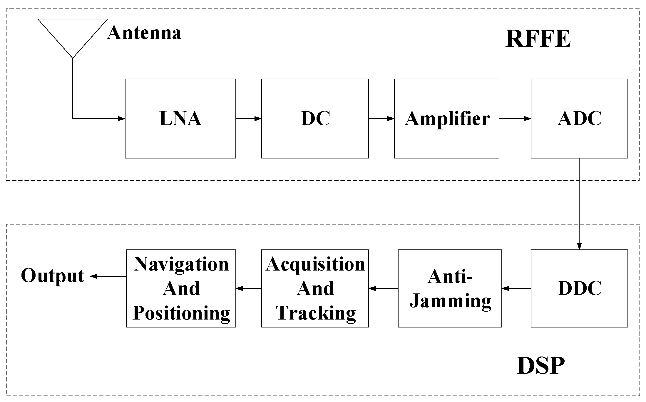
2.1. Navigation Receiver Model

The structure of a satellite navigation receiver includes two parts: radio frequency front-end (RFFE) processing and baseband digital signal processing (DSP) [26]. Navigation receivers generally add an anti-jamming module to suppress interference such as narrow-band interference [27]. As shown in Figure 1, the receiver RFFE performs analog signal processing on the antenna received signal, including low-noise amplifier (LNA), down-conversion (DC), amplifier, and analog to digital converter (ADC). The baseband DSP includes digital down-conversion (DDC), anti-jamming, acquisition and tracking, navigation, and positioning [28].
Suppose that the intermediate frequency (IF) signal, noise, and interference received from an antenna and processed after DDC are s [ n ] , n [ n ] and j [ n ] , respectively, and they are all complex signals [29]. Then the signal before anti-jamming can be expressed as [27].
x [ n ] = s [ n ] + j [ n ] + n [ n ]
The carrier-to-noise ratio (CNR) is an essential parameter for evaluating navigation signal quality. Different from communication systems, navigation systems take ranging and positioning as the ultimate goal [30,31]. Therefore, the CNR can evaluate the receiver performance while there is no need to consider the decoding processing as performed in communication systems [32]. The ideal CNR after the anti-jamming filter is the CNR without interference, which can be expressed as [6].
[ C / N ] 0 = C N B N = S s ( f ) d f S n ( f ) d f B n ,
where S s ( f ) and S n ( f ) are the power spectral densities of the IF signal and noise, respectively.
The weight vector of an anti-jamming filter can be defined by [28].
W M = [ w 0 , w 1 , , w M ] ,
where M is the order of the time domain filter, then the filter length can be expressed as [33].
N = M + 1
The output signal after the anti-jamming filter can be expressed in the time domain as [33].
y [ n ] = x [ n ] W M = k = 0 M x [ n k ] W M [ k ]
The frequency response of the anti-jamming filter can be written as [33].
H ( f ) = DTFT [ W M ]
The estimated CNR after anti-jamming is a vital indicator to estimate the interference suppression performance, which can be expressed as [6].
[ C / N ] ajm = | H ( f ) | 2 S s ( f ) d f S y ( f ) d f | H ( f ) | 2 S s ( f ) d f

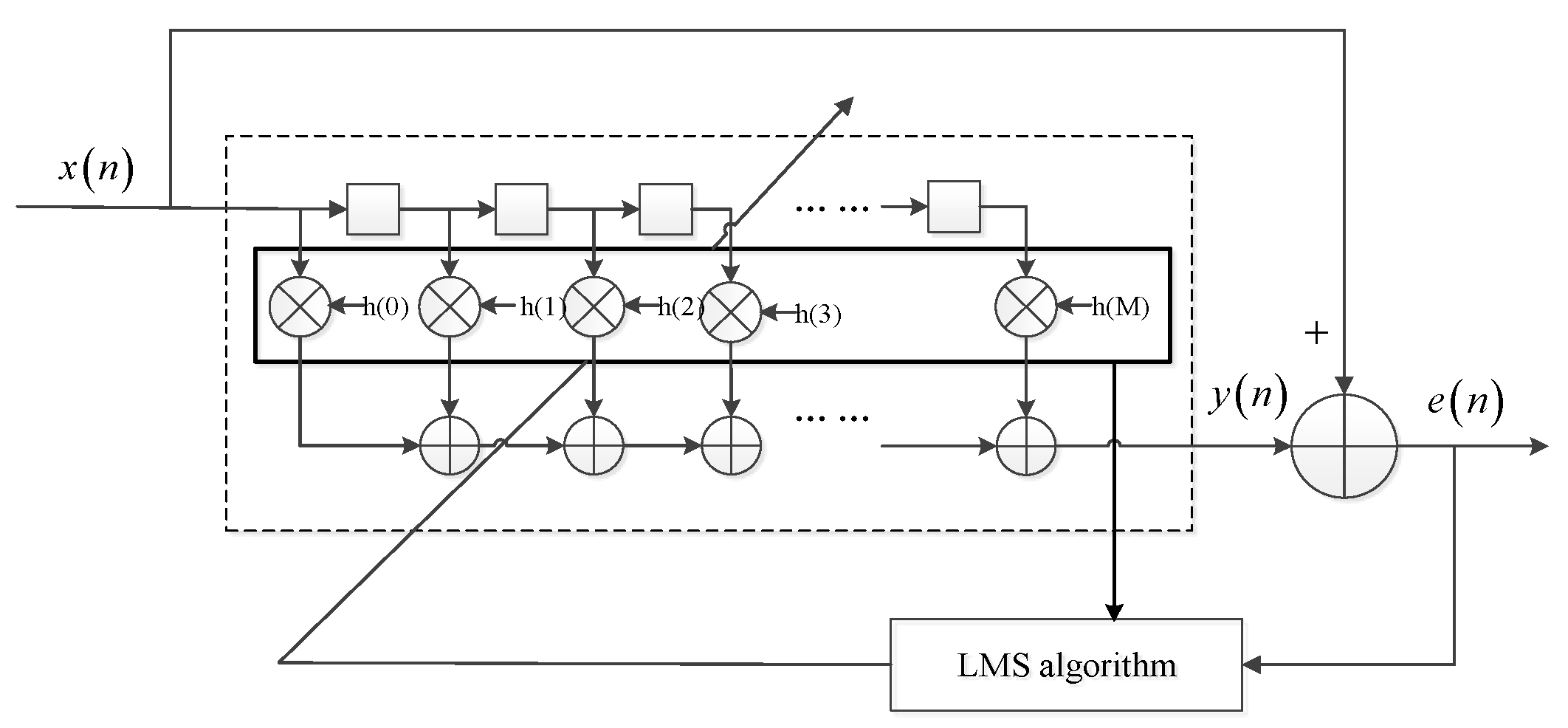
2.2. Time Domain Adaptive Anti-Jamming Filter Model

The time-domain adaptive anti-jamming technology can achieve good interference suppression performance for narrow-band interference, and it can be embedded in navigation receiver DSP independently with a small processor [33]. The classical least-mean-square (LMS) algorithm is used most often in adaptive filters because of its characteristics of small calculation and simple implementation, which uses MMSE as the optimal criterion and the steepest descent of the gradient to minimize the mean square of the error signal [34].
However, increasing the filter length cannot guarantee the improvement of anti-jamming performance for a classical LMS filter. The iteration step limits the effect of filter order on anti-jamming performance. In terms of the general relationship, as the order increases, the filter transition band is compressed, the null is deepened to obtain better interference suppression performance, and the room for improvement of higher performance will gradually be limited in the meantime. Therefore, the estimated CNR increases rapidly with the filter order and then tends to be stable with no significant increase. However, the steady-state error of the interference suppression performance is also affected by the iteration step, the convergence condition of which is inversely proportional to the filter order. Therefore, with the same iteration step, the interference suppression performance of adaptive filters does not increase monotonically with the filter order, but there are inevitable fluctuations, as shown in Figure 2.
In this paper, the LMS algorithm of filter vectors’ zero-padding iteration can be used to alleviate the insufficient convergence of the adaptive algorithm, facilitating studying the relationship between the anti-interference performance and filter order, the structure of which is shown in Figure 3.
The error signal between the filter output signal and the input signal is defined as e ( n ) ,which can be expressed as [21].
e [ n ] = x [ n ] y [ n ]
The adaptive algorithm adjusts the filter coefficients W M according to the error signal and filter order, and the gradient vector of the mean square error can be expressed as [21].
W M E { | e [ n ] | 2 } = 2 R X W M 2 r X d ,
Suppose that the initial value of W M is set to W M , 0 , and the filter weight vector change iteratively along the negative gradient direction by the step μ , which can be expressed as [21].
W M l + 1 = W M l μ W M E { | e [ n ] | 2 } ,
where l is the number of adaptive iterations, and the maximum number of iterations is L . Different from the classical LMS algorithm, the initial value of the weight vector is obtained by the adaptive weight vector after the convergence of the filter of M 1 orders.
W M , 0 = [ 0 W M 1 , L 0 ] ,
where the initial number of the filter order is the minimum value of 2.
Substituting Formula (9) into Formula (10) to get [21].
W M l + 1 = ( I 2 μ R X ) W M l + 2 μ r X d
In practical applications, the instantaneous mean square error is usually used instead of the mean square error, and finally the recursive formula of the LMS algorithm can be obtained [21].
W M l + 1 = W M l + 2 μ e [ n ] x [ n ]

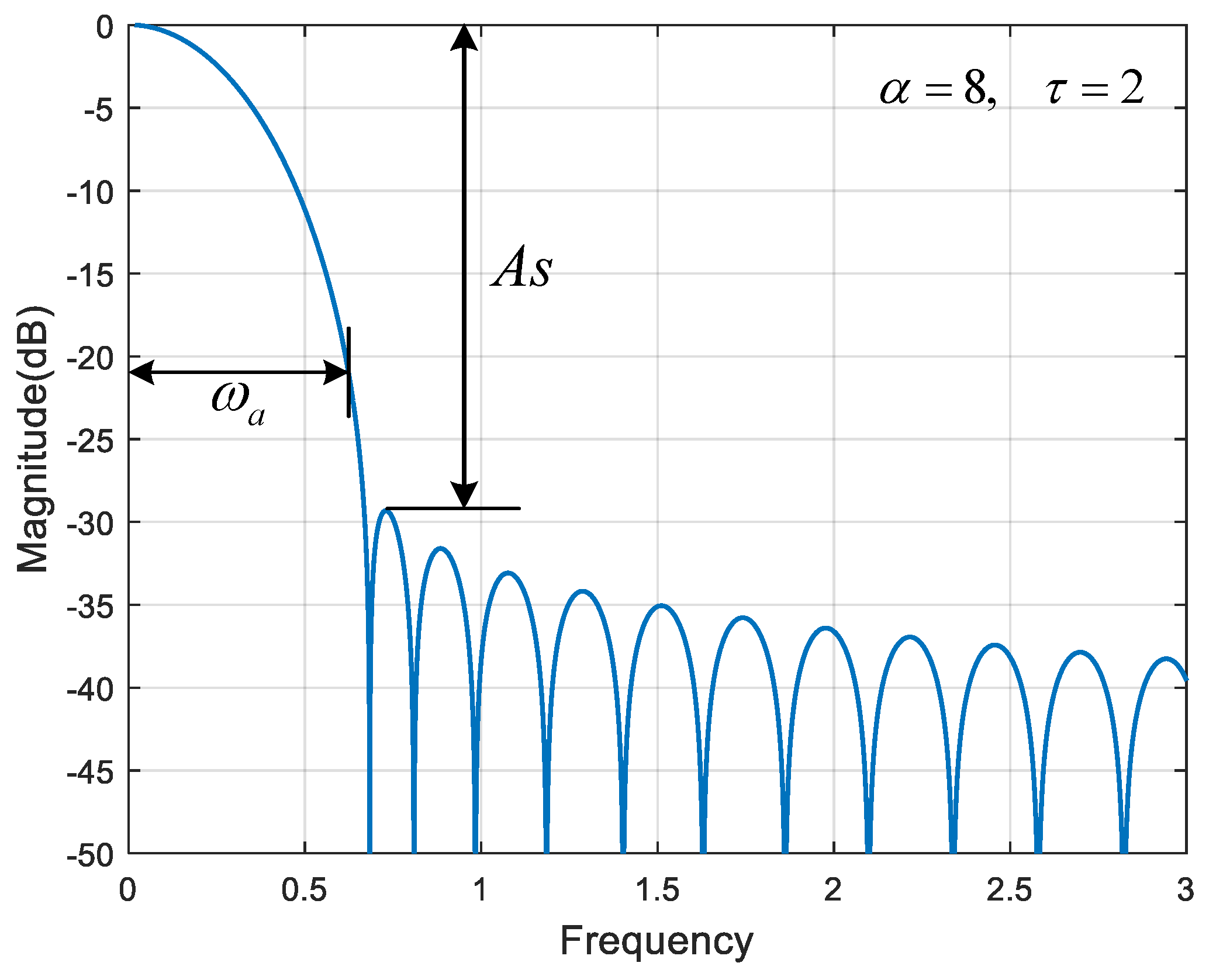
3. Analysis of Filter Order

The purpose of the study is to adaptively design the shortest anti-jamming filter according to interference characteristics, which should meet specifications requirements in the meantime. Since the algorithm parameters cannot be set directly according to the interference, the window function changing with interferences can be used to design a filter to achieve interference suppression.
The method by window function is a time-domain design method for digital filters. By adopting window functions with different finite time widths to cut the infinite length sequence, the finite length sequence is obtained, and the corresponding FIR filter is realized. The most basic window function is a rectangular window [35]. By weighting the amplitude of the rectangular window function, more window functions with different performances can be obtained, such as triangular window, Hanning window, Hamming window, Blackman window, and Kaiser window. Kaiser window can adjust the width of the main lobe and the attenuation of the side lobe by restricting filter length, which means it has good adaptability to the interference of different power and bandwidth [36]. Other window functions cannot control the filter performance as flexibly as the Kaiser window. Therefore, the Kaiser window is most suitable for calculating the optimal filter order.
The Kaiser window comprises Bessel functions and contains complex and variable window parameters α , but it can achieve the steepest window function transition zone with the same performance. The Kaiser window function can be expressed as [37].
ω ( n ) = I 0 ( α 1 ( 1 2 n N 1 ) 2 ) I 0 ( α ) , n = 0 , 1 , , N 1 ,
The Fourier transform of Kaiser window function can be derived to be [37].
W ( ω ) = { 2 τ sinh [ α 1 ( ω / ω a ) 2 ] I 0 [ α ] α 1 ( ω / ω a ) 2 | ω | ω a 2 τ sin [ α ( ω / ω a ) 2 1 ] I 0 [ α ] α ( ω / ω a ) 2 1 | ω | > ω ,
where, α = ω a τ , f a = ω / 2 π , and I 0 ( x ) is the zero-order first-class modified Bessel function, which is defined as:
I 0 ( x ) = 1 + k = 1 [ ( x / 2 ) k k ! ] 2 ,
A typical Fourier transform of a Kaiser window (for α = 8 , τ = 2 ) is shown in Figure 4. The normalized window width is the precise transition zone of the Kaiser window, which is normalized by the product of the window width and the transition zone.
D = Δ f ( 2 τ ) ,
where Δ f is the transition bandwidth and 2 τ is the window span, which are defined as follows.
Δ f = f s f p ,
2 τ = N 1 f s ,
where f s is the stop-band cut-off frequency, and f p is the pass-band cut-off frequency.
α is a parameter for adjusting the shape of the Kaiser window. The larger α , the narrower the window width and the increase of the main lobe width. Both α and the normalized window width D can all be expressed by the minimum stop-band attenuation [38].
α = { 0.1102 ( A s 8.7 ) , A s > 50 0.5842 ( A s 21 ) 0.4 + 0.07886 ( A s 21 ) , 21 < A s < 50 0         , A s < 21 ,
D = { ( A s 7.95 ) / 14.36 A s > 21 0.9222 e l s e ,
The optimal filter order of the filter designed by the Kaiser window can be obtained by Formula (19) and Formula (21).
N = A s 7.95 14.36 ( Δ f / f s )

4. Optimal Filter Order

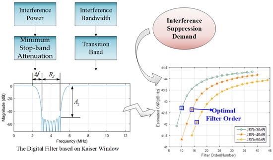
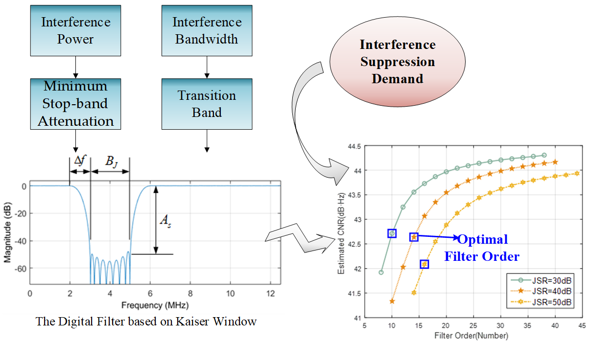
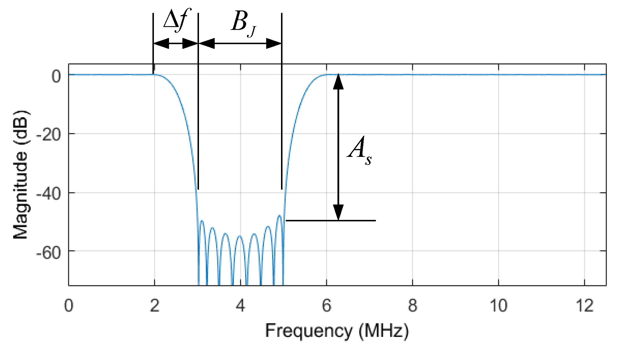
4.1. Demand Analysis of Anti-Jamming Filter

Interference suppression performance is a significant indicator of anti-jamming satellite navigation receivers [39]. CNR is usually used to access the interference suppression ratio and loss of signals resulting from the anti-jamming filter [40].
The interference suppression performance of time-domain adaptive anti-jamming filters differ from different interference characteristic of power and interference bandwidth, and its ultimate anti-jamming performance can use the maximum estimated CNR as the equivalent. The adaptive algorithm correlates signal characteristics in the time domain and forms a null in the frequency band where the interference signal is located [41]. A deeper null means a more excellent interference rejection ratio, and a narrower transition bandwidth indicates less loss of the navigation signal.
JSR (Jamming-to-Signal Ratio) and interference bandwidth are two characteristic parameters of interference signals, and these two parameters can be estimated effectively by existing corresponding algorithms in the navigation receiver [42,43]. In this paper, they are assumed to be known parameters. The difference between interference signals’ peak power and spread spectrum signals’ level is defined as the jam-to-signal ratio, and the bandwidth of the narrow-band interference can be expressed as.
B J = η ( 2 F c ) ,
where η is the interference relative bandwidth, 2 F c is the signal bandwidth, and F c is the frequency of pseudo random noise (PRN) code. While the interference relative bandwidth is less than 20%, the interference is a narrow-band interference signal [5].
The requirements of filters for suppressing various narrow-band interferences are analyzed. The simulation results shown in Figure 5 illustrate the frequency spectrum of navigation signals before and after anti-jamming, with different JSR and interference bandwidths. In order to show the bandwidth relationship between interference and receiver, the negative frequency is retained in Figure 5. There is no symmetry in the spectrum since all received signals are complex signals.
When the filter length is increased sufficiently, the anti-jamming performance can be effectively improved. However, while the filter order has become overlarge, the room for improvement in interference suppression performance is gradually compressed. In Figure 5a–c are the spectrograms before and after the anti-jamming module of different length filters: When the filter length increases from 9 to 19, the null is deepened, and the transition band is narrowed, which means that the interference suppression is enhanced while the signal loss is reduced. When the filter length increases from 19 to 29, the performance improvement is not as apparent as before. That is, e improvement of interference suppression performance is reduced.
The higher the interference signal power, the worse the interference suppression performance of the same length filter and the lower the ultimate performance the finite-length filter can achieve. Figure 5c,d are the before and after anti-interference spectrum of the filter order under interferences of different power. While the interference power increases, there is no apparent change in the null depth, but the transition band is widened. The increase in navigation signal loss leads to a decrease in anti-jamming performance.
As the interference relative bandwidth increases, the loss of navigation signals increases, resulting in a more obvious reduction in the anti-jamming performance. Therefore, the ultimate performance of the adaptive filter is reduced gradually. Pictures (c), (e), (f) are the spectrum diagrams before and after the anti-jamming filter under different bandwidth interference. The increase of interference bandwidth will not significantly impact the transition band and null of the filter frequency response. However, the anti-jamming performance will worsen because of the loss of navigation signal and additive noise in the interference suppression frequency band, and the ultimate performance will also be reduced in the meantime.

4.2. Design of Optimal Filter

The anti-jamming filter of navigation receivers is usually a band-stop filter, as shown in Figure 6, and its minimum stop-band attenuation can be expressed as the interference signal ratio.
A s = J S R
The transition band of the filter obtained from Formula (22) can be expressed as.
Δ f = D f s N 1 = { ( A s 7.95 ) f s 14.36 ( N 1 ) , A s > 21 0.922 f s N 1 , e l s e
Suppose that the center frequency of interference is f J , then the normalized upper and lower cutoff frequencies of the filter can be defined as.
ω a 1 = 2 π ( f J 1 2 B J 1 2 Δ f ) / f s ,
ω a 2 = 2 π ( f J + 1 2 B J + 1 2 Δ f ) / f s
The ideal anti-jamming filter frequency response can be defined as.
H d ( ω ) = { e j ω N 1 2 , { 0 | ω | ω a 1 } { ω a 2 | ω | π } 0     , ω a 1 < | ω | < ω a 2 ,
The frequency response of the anti-jamming filter is.
H ( f ) = ω = 2 π f 1 2 π [ H d ( ω ) W ( ω ) ] ,
When the filter length increases, the estimated CNR will get close to the ideal CNR, which means the shortest filter can be designed to meet the demand for anti-jamming. The anti-jamming requirement is the maximum acceptable CNR loss, represented by 3 dB·Hz in simulations and 8 dB·Hz in practical tests. When the difference between the C/N ratio under non-interference conditions and the estimated C/N ratio after anti-jamming is less than 3 dB·Hz, the anti-interference requirements are met.
Δ C N R = [ C / N ] 0 [ C / N ] ajm = 10 lg { B n S s ( f ) d f ( S y ( f ) d f | H ( f ) | 2 S s ( f ) d f ) S n ( f ) d f | H ( f ) | 2 S s ( f ) d f }
M min = min { M | Δ C N R 3 dB } ,
The optimal order of the time-domain adaptive filter is.
M min = min { M | Δ C N R 3 dB } + Δ M ,
where Δ M is the correction value between the optimal order obtained by theoretical derivation and design and the actual optimal filter order.

5. Experimental and Analysis

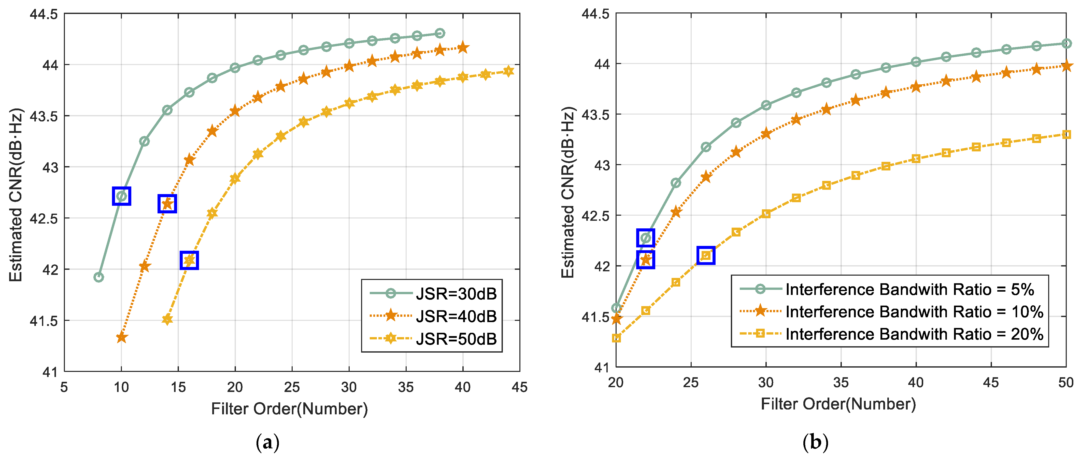
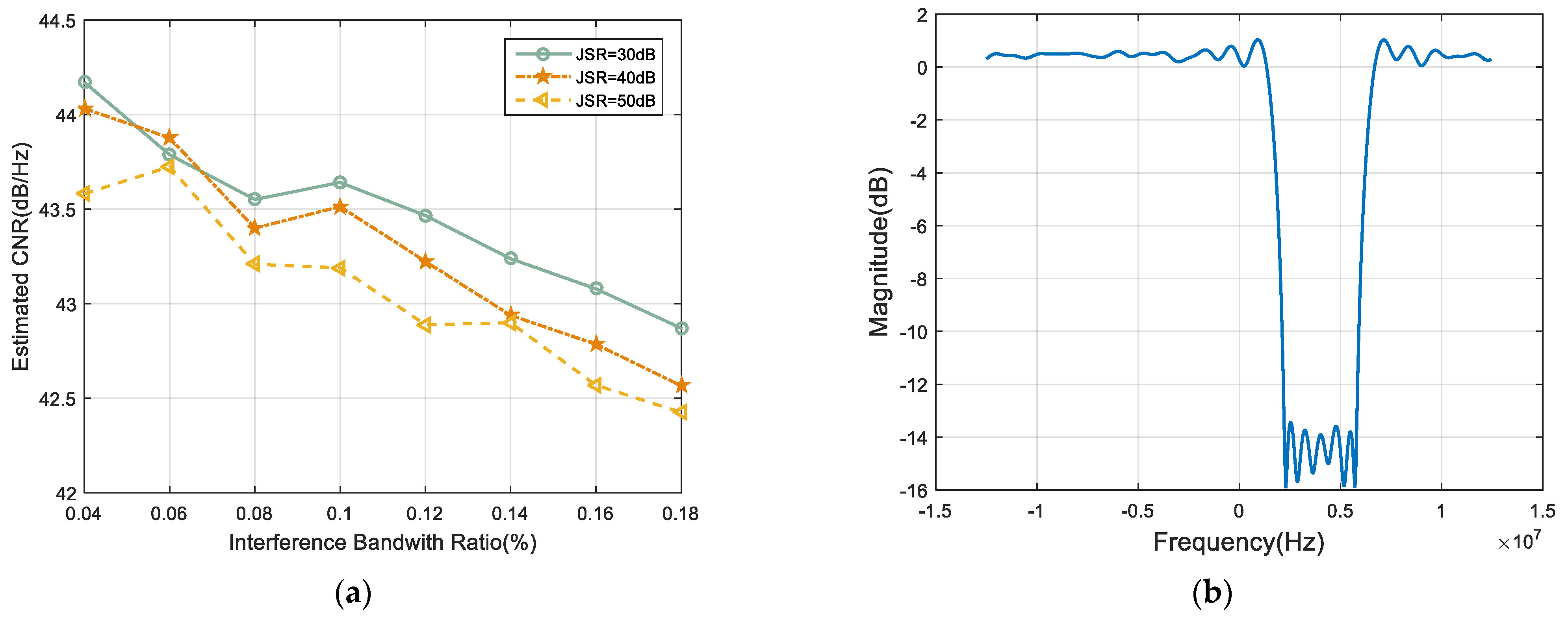
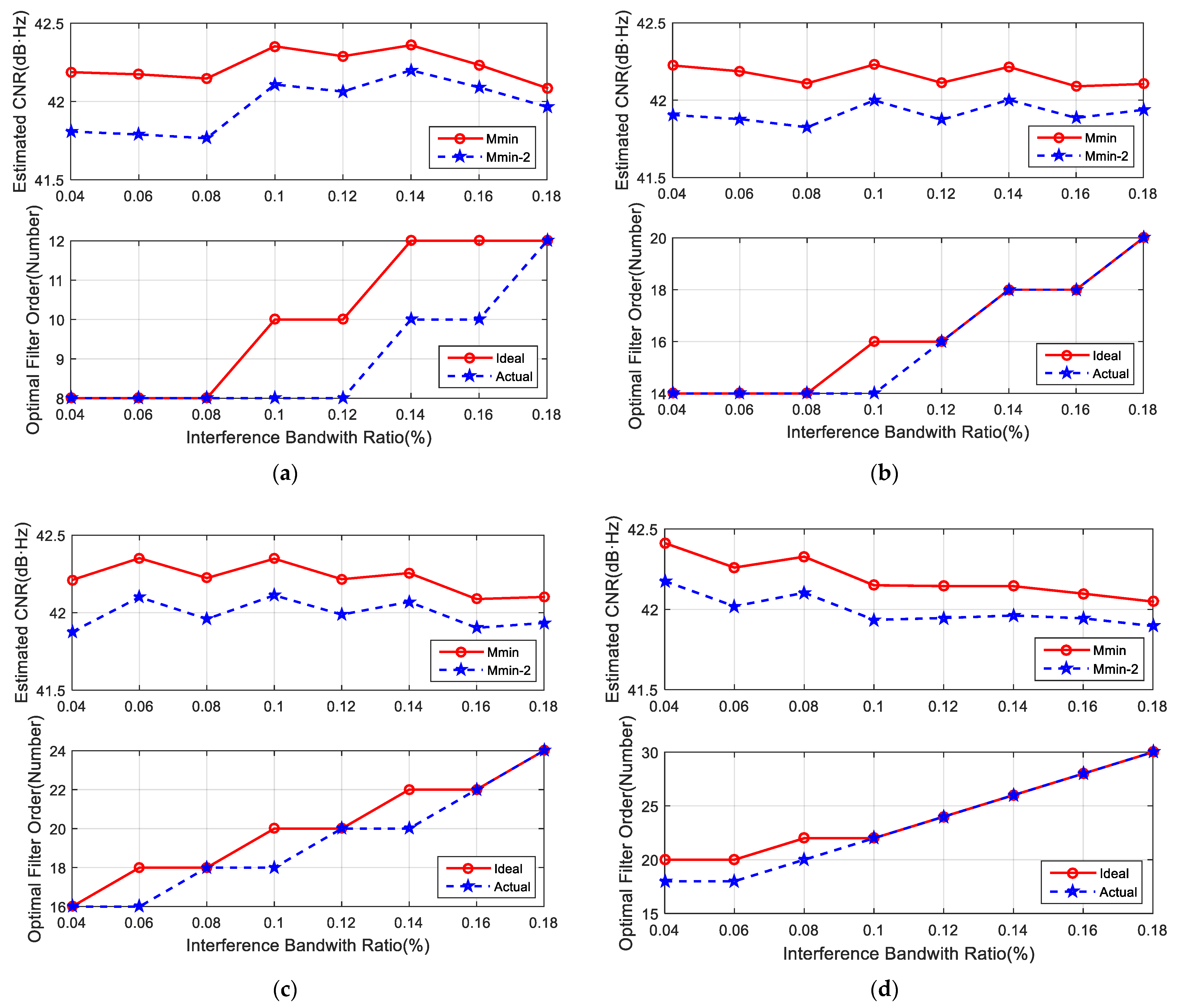
5.1. Simulation and Analysis

The simulation experiment is conducted in a software receiver composed of data generation, anti-jamming, and performance evaluation. The length of navigation signal data is set to 1 s, and the sampling rate is set to 25 MHz. The narrowband interference bandwidth differs from 5% to 15% of the PRN code bandwidth. The modulation method is P-code BPSK modulation. That is, the PRN code rate is 10.23 MHz. Set the intermediate carrier frequency to be the same as the narrowband interference center frequency, and the interference signal ratio ranges from 30 dB to 50 dB.
Figure 7a,b verify the monition increasing relation between the interference suppression performance and the filter order. As the anti-jamming filter extends, the estimated CNR increases, suggesting that more extended filters can generate better interference suppression performance. While the filter order continued to increase, the growth rate of CNR slowed down. Figure 7a is the influence of filter order on the CNR under different JSR. For the same length filter, the greater the interference power, the smaller the estimated CNR, and the ultimate performance achieved by the finite-length filter is inversely proportional to JSR. Figure 7b shows the effect of filter order on CNR under different bandwidth interference. For the same length filter, the larger the interference signal bandwidth, the smaller the estimated CNR, and the ultimate anti-jamming performance of adaptive filters decreases as the interference bandwidth increases.
The simulation obtains the optimal filter order for the interference suppression of anti-jamming filters designed by the Kaiser window function, and the Monte Carlo simulations are carried out 100 times. Figure 8 verify the interference suppression performance of the Wiener filter under the calculated optimal order. As shown in Figure 7, the estimated CNR after the Wiener filter of calculated optimal order can meet the anti-jamming demand for navigation receiver, and the room for filter shortened decreases with the increase of interference bandwidth.
Due to the limitation of algorithm parameters, the adaptive filter may not necessarily converge to the Wiener solution, resulting in the actual optimal filter order of adaptive filters being longer than the Winner solution. Besides, there are generally differences in the performance between the LMS adaptive filter and the Kaiser one because of the different design principles. Therefore, there is an error between the calculated optimal filter order and the actual value. When the JSR is 30 dB, the calculated optimal filter order can meet the interference suppression demand of adaptive filters. When the JSR increases, the gap between the calculated optimal filter order and the actual optimal filter order increases. The optimal order of the corrected time-domain adaptive filter is:
M min = { min { M | Δ C N R 3 dB } , J S R 30 dB min { M | Δ C N R 3 dB } + 4 , 30 dB < J S R < 40 dB min { M | Δ C N R 3 dB } + 6 , 40 dB J S R 50 dB ,
Figure 9 illustrates the performance comparison between the actual optimal filter order and the calculated value. It is shown that the interference suppression requirements can be well met by designing digital filters based on the Kaiser window.

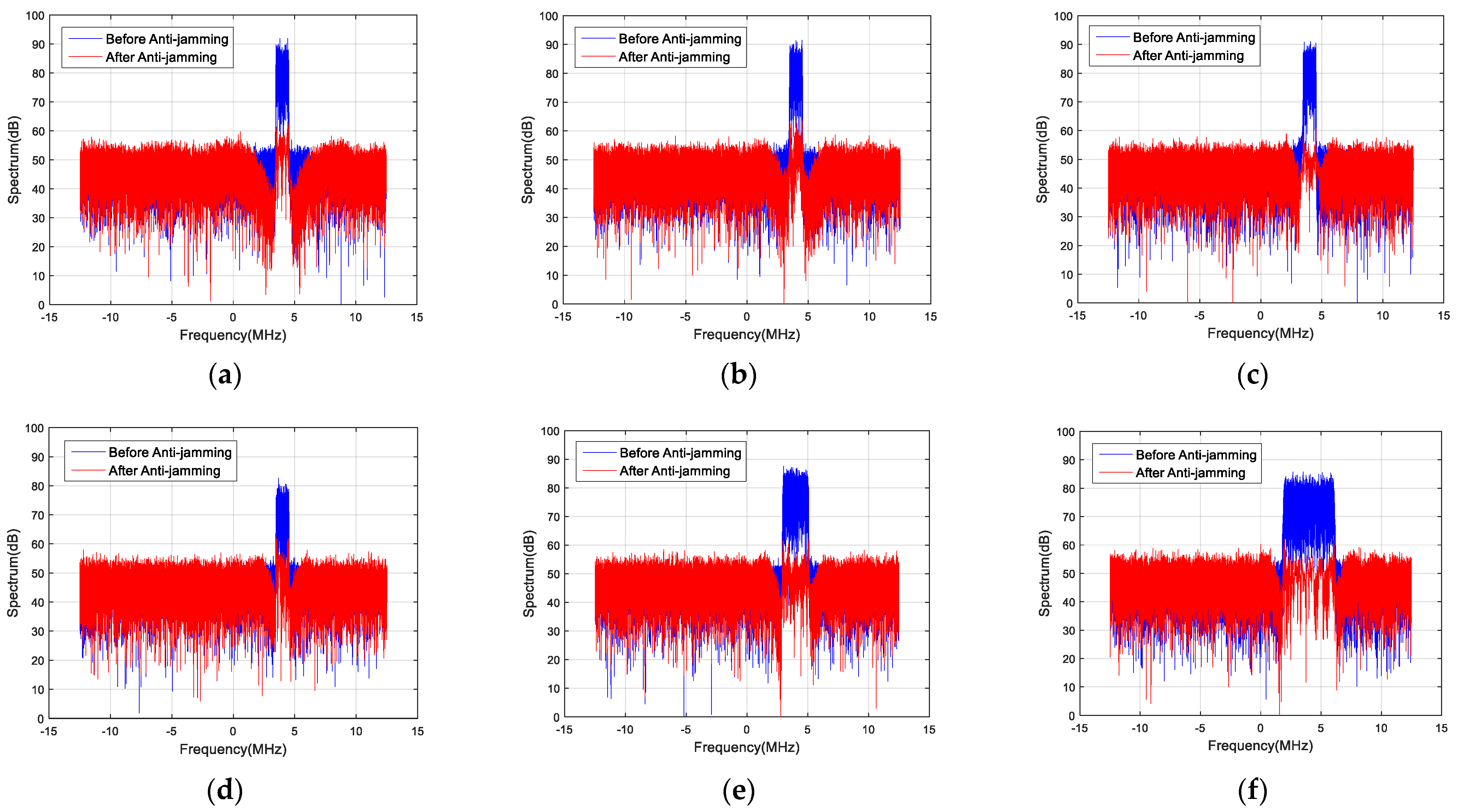
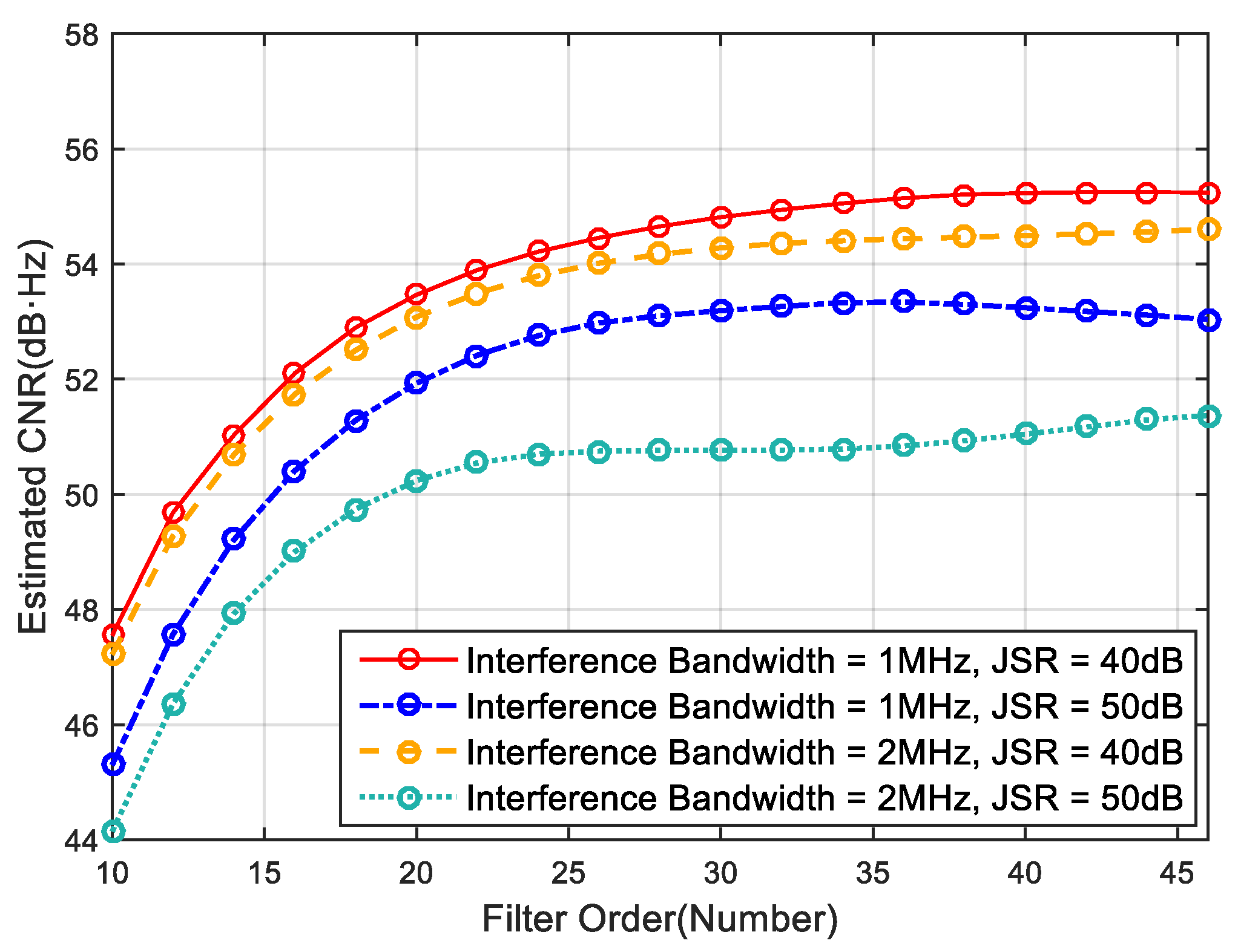
5.2. Measured Data Analysis

A practical test was performed in a controlled environment with interference sources of different power and bandwidth to verify the applicability of this approach in GNSS receivers’ real-world scenarios. The interference source controls the power and bandwidth of interference signals, and the desired navigation signal is a Beidou B3 civil signal originating from the No.7 satellite. Our experimental platform is depicted in Figure 10.
The parameters of the practical test are as follows: the data length is 1 ms; the sampling rate is 75.12 MHz; the receiver’s bandwidth is 20 MHz; the correction value Δ M is set to be 0; the maximum CNR loss for designing the optimal filter order is 8 dB·Hz; the CNR of undisturbed signals is 58 dB·Hz. This paper adopts six interference scenes.
Scene 1.
Set interference bandwidth to 2 MHz, and JSR to approximately 50 dB.
Scene 2.
Set interference bandwidth to 2 MHz, and JSR to approximately 40 dB.
Scene 3.
Set interference bandwidth to 1 MHz, and JSR to approximately 50 dB.
Scene 4.
Set interference bandwidth to 1 MHz, and JSR to approximately 40 dB.
Scene 5.
Set interference to be single-frequency interference, and JSR to approximately 50 dB.
Scene 6.
Set interference to be single-frequency interference, and JSR to approximately 40 dB.
The interference suppression performance for the above six scenarios is shown in Table 1, which shows that the CNR loss with optimal filter order under real-world scenarios is less than 8 dB·Hz, and the optimal filter order increases with the bandwidth and power of the interference signal. Besides, the CNR loss (<8 dB·Hz) also increases with the interference power, which means that the error between calculated optimal filter order and actual filter order is minor for larger interference bandwidth and JSR. The results from signal-frequency signals show that this approach is more suitable for narrow-band interference suppression.
Figure 11 illustrates the estimated CNR for the four narrow-band interference suppression scenes. The interference suppression performance increases and tends to be stable with the adaptive filter tap-length increases, accompanied by a slight decrease trend. By comparing Table 1 and Figure 11, it can be found that the calculated optimal filter order is much larger than the actual one under the practical test. In all cases, the sampling rate is 75.12 MHz, larger than the Nyquist frequency, which results in the anti-jamming adaptive filter designed through Kaiser-window longer than the actual optimal filter.
In conclusion, we have demonstrated that the narrowband interference embedded in navigation signals can be suppressed by the adaptive LMS filter with optimal tap-number, ensuring a short filter to meet the anti-interference requirements of the navigation receiver. However, this method needs to limit the sampling rate as close to the Nyquist sampling rate as possible, especially in practical receiver applications.

6. Conclusions

The optimal time-domain adaptive anti-jamming filter based on the Kaiser window method is proposed by analyzing the effect of the adaptive filter order on interference suppression performance and hardware occupancy of navigation receivers. With no need for detailed information of navigation interference, but only the interference bandwidth and JSR, the filter designed by the Kaiser window can be used to obtain the optimal order to meet the anti-jamming requirements, and the calculated optimal filter order is corrected according to the test data. The algorithm is simplified by the FIR filter design method, without knowing the specific information of interferences, and the convergence process of the adaptive algorithm is avoided, the time cost significantly reduced, the accuracy of the optimal order selection ensured. Through simulation analysis and practical tests, the following conclusions have been obtained:
(1)
A higher power interference scenery requires a larger optimal filter order to meet the time-domain adaptive anti-jamming requirements.
(2)
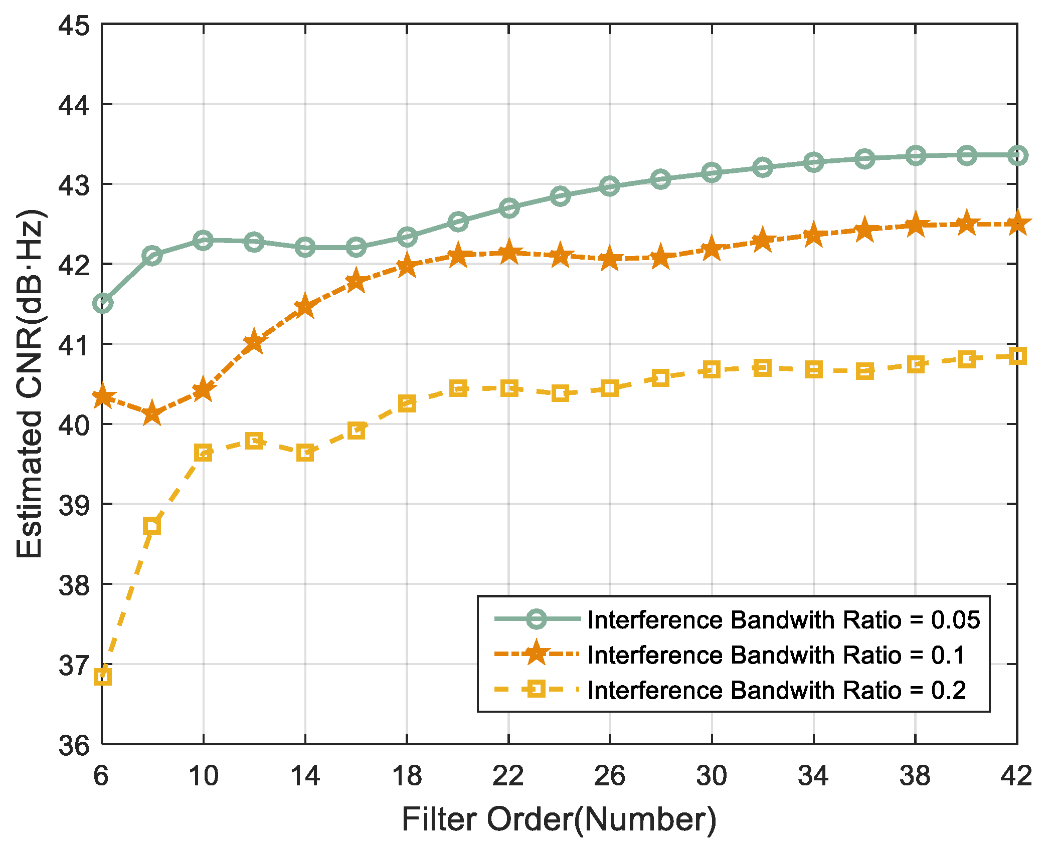
A more expansive bandwidth interference scenery requires a larger optimal filter order to meet the time-domain adaptive anti-jamming requirements.
(3)
The time-domain adaptive filter can meet navigation receivers’ 3 dB·Hz anti-jamming requirement in simulations and 8 dB·Hz requirement in practical tests with the optimal filter order.

Author Contributions

J.S. performed the theoretical study, conducted the experiments, processed the data and wrote the manuscript. Z.L. designed the system, provided research suggestions and revised the manuscript together with Z.X. and Z.X. helped in performing the experiments. B.L. and G.S. provided the experiment equipment and suggestions for the manuscript. All authors have read and agreed to the published version of the manuscript.

Funding

This research was funded by the National Natural Science Foundation of China (No.62003354).

Institutional Review Board Statement

Not applicable.

Informed Consent Statement

Not applicable.

Data Availability Statement

No date supporting.

Acknowledgments

The authors would like to thank the editors and reviewers for their efforts to help the publication of this paper.

Conflicts of Interest

The authors declare no conflict of interest.

References

  1. Chen, Y.-H.; Juang, J.-C.; Seo, J.; Lo, S.; Akos, D.M.; De Lorenzo, D.S.; Enge, P. Design and Implementation of Real-Time Software Radio for Anti-Interference GPS/WAAS Sensors. Sensors 2012, 12, 13417–13440. [Google Scholar] [CrossRef] [Green Version]
  2. Zhang, J.; Cui, X.; Xu, H.; Lu, M. A Two-Stage Interference Suppression Scheme Based on Antenna Array for GNSS Jamming and Spoofing. Sensors 2019, 19, 3870. [Google Scholar] [CrossRef] [Green Version]
  3. Lu, Z.; Nie, J.; Wan, Y.; Ou, G. Optimal reference element for interference suppression in GNSS antenna arrays under channel mismatch. IET Radar Sonar Navig. 2017, 11, 1161–1169. [Google Scholar] [CrossRef]
  4. Zhang, P.; Tu, R.; Zhang, R.; Gao, Y.; Cai, H. Combining GPS, BeiDou, and Galileo Satellite Systems for Time and Frequency Transfer Based on Carrier Phase Observations. Remote Sens. 2018, 10, 324. [Google Scholar] [CrossRef] [Green Version]
  5. Loh-Ming, L.; Milstein, L. Rejection of Narrow-Band Interference in PN Spread-Spectrum Systems Using Transversal Filters. IEEE Trans. Commun. 1982, 30, 925–928. [Google Scholar] [CrossRef]
  6. Shi, K.; Jia, Y.; Fu, S.; Cao, Z.; Chen, P. Adaptive Narrowband Antijam Method for Satellite Navigation. In Proceedings of the 2018 International Conference on Electromagnetics in Advanced Applications (ICEAA), Cartagena De Indias, Colombia, 10–14 September 2018; pp. 687–690. [Google Scholar]
  7. Chia-Lung, C.; Fan-Ren, C.; Kun-Yuan, T. Highly accurate real-time GPS carrier phase-disciplined oscillator. IEEE Trans. Instrum. Meas. 2005, 54, 819–824. [Google Scholar] [CrossRef]
  8. Zhang, Y.; Kubo, N.; Chen, J.; Wang, J.; Wang, H. Initial Positioning Assessment of BDS New Satellites and New Signals. Remote Sens. 2019, 11, 1320. [Google Scholar] [CrossRef] [Green Version]
  9. Yang, H.; Zhou, B.; Wang, L.; Wei, Q.; Ji, F.; Zhang, R. Performance and Evaluation of GNSS Receiver Vector Tracking Loop Based on Adaptive Cascade Filter. Remote Sens. 2021, 13, 1477. [Google Scholar] [CrossRef]
  10. Gong, Y.; Cowan, C.F.N. A novel variable tap-length algorithm for linear adaptive filters. In Proceedings of the 2004 IEEE International Conference on Acoustics, Speech, and Signal Processing, Montreal, QC, Canada, 17–21 May 2004; p. ii-825. [Google Scholar]
  11. Lu, Z.; Chen, F.; Xie, Y.; Liu, Z. Impact on Anti-jamming Performance of GNSS Signal Bandwidth under Channel Mismatch Used Antenna Arrays. In Proceedings of the 2020 5th International Conference on Computer and Communication Systems (ICCCS), Shanghai, China, 15–18 May 2020. [Google Scholar]
  12. Xu, W.; Xing, W.; Fang, C.; Huang, P.; Tan, W.; Gao, Z. RFI Suppression for SAR Systems Based on Removed Spectrum Iterative Adaptive Approach. Remote Sens. 2020, 12, 3520. [Google Scholar] [CrossRef]
  13. Zhou, Q.; Zheng, H.; Wu, X.; Yue, X.; Chen, Z.; Wang, Q. Fractional Fourier Transform-Based Radio Frequency Interference Suppression for High-Frequency Surface Wave Radar. Remote Sens. 2020, 12, 75. [Google Scholar] [CrossRef] [Green Version]
  14. Zhao, H.; Hu, Y.; Sun, H.; Feng, W. A BDS Interference Suppression Technique Based on Linear Phase Adaptive IIR Notch Filters. Sensors 2018, 18, 1515. [Google Scholar] [CrossRef] [PubMed] [Green Version]
  15. Widrow, B.; McCool, J.M.; Larimore, M.G.; Johnson, C.R. Stationary and nonstationary learning characteristics of the LMS adaptive filter. Proc. IEEE 1976, 64, 1151–1162. [Google Scholar] [CrossRef]
  16. Chern, S.; Sun, C. Linearly constrained RLS algorithm with variable forgetting factor for DS-CDMA system. In Proceedings of the 2014 International Symposium on Intelligent Signal Processing and Communication Systems (ISPACS), Kuching, Sarawak, Malaysia, 1–4 December 2014; pp. 261–264. [Google Scholar]
  17. Lee-Min, L.; Hsiao-Chuan, W. An extended Levinson-Durbin algorithm for the analysis of noisy autoregressive process. IEEE Signal Process. Lett. 1996, 3, 13–15. [Google Scholar] [CrossRef]
  18. Burg, J.P. Maximum Entropy Spectral Analysis; Stanford University: Stanford, CA, USA, 1975. [Google Scholar]
  19. Vijayan, R.; Poor, H.V. Nonlinear techniques for interference suppression in spread-spectrum systems. IEEE Trans. Commun. 1990, 38, 1060–1065. [Google Scholar] [CrossRef]
  20. Chong, Z.; He, H.; Haisong, J.; Qingliang, C.; Qing, G.; Feng, L.; Li, S. Research on Anti-jamming algorithm and performance of array antenna. In Proceedings of the 2018 IEEE CSAA Guidance, Navigation and Control Conference (CGNCC), Nanjing, China, 10–12 August 2018; pp. 1–5. [Google Scholar]
  21. Yuantao, G.; Kun, T.; Huijuan, C. LMS algorithm with gradient descent filter length. IEEE Signal Process. Lett. 2004, 11, 305–307. [Google Scholar] [CrossRef]
  22. Riera-Palou, F.; Noras, J.M.; Cruickshank, D.G.M. Linear equalisers with dynamic and automatic length selection. Electron. Lett. 2001, 37, 1553. [Google Scholar] [CrossRef]
  23. Yu, G.; Cowan, C.F.N. An LMS style variable tap-length algorithm for structure adaptation. IEEE Trans. Signal Process. 2005, 53, 2400–2407. [Google Scholar] [CrossRef] [Green Version]
  24. Wei, Y.; Yan, Z. Variable Tap-Length LMS Algorithm with Adaptive Step Size. Circuits Syst. Signal Process. 2017, 36, 2815–2827. [Google Scholar] [CrossRef]
  25. Akhtar, M.T.; Ahmed, S. A robust normalized variable tap-length normalized fractional LMS algorithm. In Proceedings of the 2016 IEEE 59th International Midwest Symposium on Circuits and Systems (MWSCAS), Monterey, CA, USA, 16–19 October 2016; pp. 1–4. [Google Scholar]
  26. Chen, F.; Nie, J.; Li, B.; Wang, F. Distortionless space-time adaptive processor for global navigation satellite system receiver. Electron. Lett. 2015, 51, 2138–2139. [Google Scholar] [CrossRef]
  27. Xie, X.; Fang, R.; Geng, T.; Wang, G.; Zhao, Q.; Liu, J. Characterization of GNSS Signals Tracked by the iGMAS Network Considering Recent BDS-3 Satellites. Remote Sens. 2018, 10, 1736. [Google Scholar] [CrossRef] [Green Version]
  28. Lu, Z.; Nie, J.; Chen, F.; Chen, H.; Ou, G. Adaptive Time Taps of STAP Under Channel Mismatch for GNSS Antenna Arrays. IEEE Trans. Instrum. Meas. 2017, 66, 2813–2824. [Google Scholar] [CrossRef]
  29. Karamalis, P.D.; Kanatas, A.G.; Constantinou, P. A Genetic Algorithm Applied for Optimization of Antenna Arrays Used in Mobile Radio Channel Characterization Devices. IEEE Trans. Instrum. Meas. 2009, 58, 2475–2487. [Google Scholar] [CrossRef]
  30. Wang, P.; Lu, X.; Wang, R. Novel narrowband jamming suppression algorithm in communication system. In Proceedings of the 2017 7th IEEE International Conference on Electronics Information and Emergency Communication (ICEIEC), Barcelona, Spain, 21–23 July 2017; pp. 95–100. [Google Scholar]
  31. Chen, M.; Liu, Y.; Guo, J.; Song, W.; Zhang, P.; Wu, J.; Zhang, D. Precise Orbit Determination of BeiDou Satellites with Contributions from Chinese National Continuous Operating Reference Stations. Remote Sens. 2017, 9, 810. [Google Scholar] [CrossRef] [Green Version]
  32. Lu, Z.; Chen, H.; Chen, F.; Nie, J.; Ou, G. Blind adaptive channel mismatch equalisation method for GNSS antenna arrays. IET Radar Sonar Navig. 2018, 12, 383–389. [Google Scholar] [CrossRef]
  33. Lu, Z.; Chen, F.; Xie, Y.; Sun, Y.; Cai, H. High Precision Pseudo-Range Measurement in GNSS Anti-jamming Antenna Array Processing. Electronics 2020, 9, 412. [Google Scholar] [CrossRef] [Green Version]
  34. Shanmugam, Y.; Subbiya, A.; Sudhakar, M.; Harsha Visali, D. Design of FIR Filter Using Adaptive LMS Algorithm for Energy Efficient Application. J. Phys. Conf. Ser. 2021, 1916, 012067. [Google Scholar] [CrossRef]
  35. Saramaki, T. A class of window functions with nearly minimum sidelobe energy for designing FIR filters. In Proceedings of the IEEE International Symposium on Circuits and Systems, Monterey, CA, USA, 8–11 May 1989; Volume 351, pp. 359–362. [Google Scholar]
  36. Andria, G.; Savino, M.; Trotta, A. Windows and interpolation algorithms to improve electrical measurement accuracy. IEEE Trans. Instrum. Meas. 1989, 38, 856–863. [Google Scholar] [CrossRef]
  37. Kaiser, J. Nonrecursive digital filter design using the I-sinh window function. Proc. IEEE 1977, 1, 20–23. [Google Scholar]
  38. Kaiser, J.; Schafer, R. On the use of the I0-sinh window for spectrum analysis. IEEE Trans. Acoust. Speech Signal Process. 1980, 28, 105–107. [Google Scholar] [CrossRef]
  39. White, N.A.; Maybeck, P.S.; DeVilbiss, S.L. Detection of interference/jamming and spoofing in a DGPS-aided inertial system. IEEE Trans. Aerosp. Electron. Syst. 1998, 34, 1208–1217. [Google Scholar] [CrossRef] [Green Version]
  40. Li, W.; Zhao, Z.; Tang, J.; He, F.; Li, Y.; Xiao, H. Performance Analysis and Optimal Design of the Adaptive Interference Cancellation System. IEEE Trans. Electromagn. Compat. 2013, 55, 1068–1075. [Google Scholar] [CrossRef]
  41. Cho, N.I.; Lee, S.U. On the adaptive lattice notch filter for the detection of sinusoids. IEEE Trans. Circuits Syst. II Analog Digit. Signal Process. 1993, 40, 405–416. [Google Scholar] [CrossRef]
  42. Sun, K.; Yu, B.; Elhajj, M.; Ochieng, W.Y.; Zhang, T.; Yang, J. A Novel GNSS Interference Detection Method Based on Smoothed Pseudo-Wigner–Hough Transform. Sensors 2021, 21, 4306. [Google Scholar] [CrossRef]
  43. Sun, K.; Zhang, T. A New GNSS Interference Detection Method Based on Rearranged Wavelet–Hough Transform. Sensors 2021, 21, 1714. [Google Scholar] [CrossRef] [PubMed]
Figure 1. Navigation receiver structure.
Remotesensing 14 00048 g001
Figure 2. Estimated CNR after anti-jamming filter of LMS algorithm.
Remotesensing 14 00048 g002
Figure 3. LMS adaptive filter of filter vectors’ zero padding iteration.
Remotesensing 14 00048 g003
Figure 4. A typical Fourier transform of Kaiser window.
Remotesensing 14 00048 g004
Figure 5. Spectrogram of navigation signals. (a) JSR = 50 dB / N = 9 / η = 0.05 ; (b) JSR = 50 dB / N = 19 / η = 0.05 ; (c) JSR = 50 dB / N = 29 / η = 0.05 ; (d) JSR = 40 dB / N = 29 / η = 0.05 ; (e) JSR = 50 dB / N = 29 / η = 0.1 ; (f) JSR = 50 dB / N = 29 / η = 0.2 .
Remotesensing 14 00048 g005
Figure 6. Frequency response of an anti-jamming filter.
Remotesensing 14 00048 g006
Figure 7. Effect of the filter orders on anti-jamming performance. (a) Impact analysis of JSR; (b) Impact analysis of Interference Bandwidth Ratio.
Remotesensing 14 00048 g007
Figure 8. Performance of Wiener filter under the calculated optimal order. (a) Interference suppression performance of Winner filter; (b) Frequency response.
Remotesensing 14 00048 g008
Figure 9. The anti-jamming performance under optimal filter order. (a) JSR = 30 dB; (b) JSR = 35 dB; (c) JSR = 40 dB; (d) JSR = 50 dB.
Remotesensing 14 00048 g009
Figure 10. Platform of the practical test.
Remotesensing 14 00048 g010
Figure 11. Effect of the filter order on narrowband interference suppression performance.
Remotesensing 14 00048 g011
Table 1. Interference Suppression Performance Comparison.
Interference SuppressionJSR (dB)Optimal Filter OrderCNR loss (dB·Hz)
Single-frequency40312.907
50413.503
1 MHz40352.726
50474.839
2 MHz40453.571
50596.198
Publisher’s Note: MDPI stays neutral with regard to jurisdictional claims in published maps and institutional affiliations.

