1. Introduction
The first static Global Navigation Satellite System (GNSS) stations have been established almost three decades ago. Today, we profit from very long observation time series, where the height component allows us to resolve important information about the vertical movement of the Earth’s crust. This movement is affected by long-term trends, linear drifts, seasonal motions, and offsets. The seasonal variations are dominated by annual and semi-annual periodicities, that can partly be explained by the so-called environmental surface loadings. These can be categorized into hydrological (HYDL), non-tidal atmospheric (NTAL), and non-tidal oceanic loading (NTOL).
Already, in 1994, van Dam et al. [
1] started analyzing the impact of atmospheric pressure on the GNSS height variance and (also van Dam et al. [
2]) correlate atmospheric and oceanic leading with geoid deformation and further with GNSS height deviations. Based on global GNSS solutions, Dam et al. [
3] also observe a correlation of continental water storage and vertical crust movement. Gegout et al. [
4] introduce environmental loadings in the processing of GNSS height solutions and are able to improve the height residuals, but mainly in the northern hemisphere. In the southern hemisphere, most of their test stations were located closer to coastal regions, and the assumption was that the missing improvement can be traced back to mis-modeled tropospheric zenith delay. Recent studies look into the comparison of different environmental surface loading models [
5,
6,
7,
8], the comparison of geophysical models and information drawn from the Gravity Recovery and Climate Experiment (GRACE) [
9], and the assimilation of both approaches [
10,
11]. Up to today, there is no standardized procedure of modeling and reducing the station position by environmental surface loadings [
12]. Most studies achieve a Root Mean Square (RMS) improvement of around 20–40%, and some suggest mis-modeled tropospheric delays as a source of the remaining height variability [
4,
12].
Machine learning has become more important in recent years and is also emerging in the field of GNSS time series analysis, including a wide range of applications [
13]. Several studies combine parameters derived from GNSS observations, such as precipitable or integrated water vapor (PVW, IVW) and meteorological data, in a deep learning approach to forecast heavy rainfall [
14,
15,
16] or to perform storm nowcasting [
17]. Another cluster of applications of using of machine learning and GNSS can be found in the modeling and prediction of tropospheric zenith delay [
18,
19,
20,
21]. In a recent study, Özdemir [
22] take the approach of machine learning, but, instead of modeling the tropospheric delay first, they directly correct the GNSS position by meteorological parameters with the help of an artificial neural network (ANN) in a real-time application.
In this study, we are working on the post-processing of the dense network of GNSS stations in central Europe. We aim to improve GNSS residual height time series, by taking into account environmental loadings and then further reduce the remaining signal. In a first step, we take the GNSS height residuals and train the TCN directly on the meteorological parameters, and then compare it with the subtraction of the physical model. In a second step, we first reduce the GNSS residuals by the environmental loading models and then train the TCN on the already reduced time series. The idea is to find a model to partly explain the remaining signal and use it to further reduce the height residuals.
2. Data and Pre-Processing
2.1. GNSS Height Residuals
The Nevada Geodetic Laboratory (NGL) collects data from all available geodetic GNSS stations worldwide and makes their station position solutions publicly available [
23]. For this work, the 24-h final solutions in the area of central Europe are used, where a network of stations with a nearby meteorological station is available (see
Section 2.3). The dataset has daily sampling, ranging from January 1994 to October 2020. Only the stations that have a time span of minimum 3.5 years and not more than 20% of missing observations are used.
Figure 1 shows the distribution and data availability of the selected NGL stations. The raw data files were downloaded from NGL (
http://geodesy.unr.edu/index.php, accessed on 13 November 2020) in
tenv3 format and further processed in the software package
Hector [
24]. Outliers are removed, and discontinuities are detected and corrected for. Then, a linear trend is fitted and subtracted, resulting in the detrended and cleaned signal.
2.2. Environmental Surface Loadings
The vertical displacements, caused by environmental surface loadings (HYDL, NTAL, NTOL), are available from the Earth System Modeling Group Repository of Deutsche Geoforschungszentrum Potsdam (ESMGFZ) [
25]. All loadings are stored in a regular 0.5
× 0.5
grid, and, while HYDL is provided in 24 h sampling, NTAL and NTOL have a 3 h sampling rate. First, NTAL and NTOL are downsampled to 24-h observation spacing by taking the daily average. In a next step, to reduce the GNSS residuals by the loading data, their values on the exact station positions are needed. These are derived from the grid by conducting a bilinear interpolation. Additionally, all resulting HYDL time series are reduced by a second-order polynomial fit, in order to correct for a second-order long-term trend, appearing at some stations. In
Figure 2, the final individual loadings, as well as the sum of them, are depicted for the example station
MAR3. More details about the preprocessing of the environmental surface loadings, as well as of the GNSS height residuals described in the previous section, can be found in Reference [
26].
2.3. Meteorological Data
Meteorological data is provided by the European Climate Assessment and Dataset (ECAD) [
27]. The dataset is downloadable as a predefined subset of daily observations, sorted by stations and parameters. The used dataset is blended, meaning that nearby stations (12.5 km distance and 25 m height difference) are used to fill any datagaps (
https://www.ecad.eu/helptext/blending_help.html, accessed on 11 December 2021). This work includes time series of the daily mean temperature (degree celcius), precipitation amount (millimeters), sea level pressure (hectopascal), humidity (percent), and radiation (Watt per square meter). In
Figure 3, all parameters are shown for the example station
MAR3. The only stations used are those where all listed parameters are available, and not more than 20% of observations are missing. In order to match GNSS and meteo stations, the closest meteorological station to GNSS station was selected, with a maximum distance of 50 km. If no suitable meteorological station could be allocated, the GNSS station had to be removed from the dataset, which led to the final distribution of used GNSS stations.
Figure 4 shows all selected meteorological and GNSS stations, as well as the distances from each GNSS station to the corresponding meteorological station.
2.4. Reduction of GNSS Residuals by Environmental Loadings
In
Figure 5, an overview of the processing steps for the reduction of GNSS residuals by environmental surface loadings is shown. The original time series (GNSS and environmental loadings) are processed individually, according to the steps highlighted in the orange boxes, to
and
. The sum of the processed loading time series
is then subtracted from
, resulting the the reduced GNSS residuals
. From
and
, the Root Mean Square reduction
is computed. In
Figure 6, the different processing steps are shown on one example station (
MAR3) from the raw data to the loading reduced residuals.
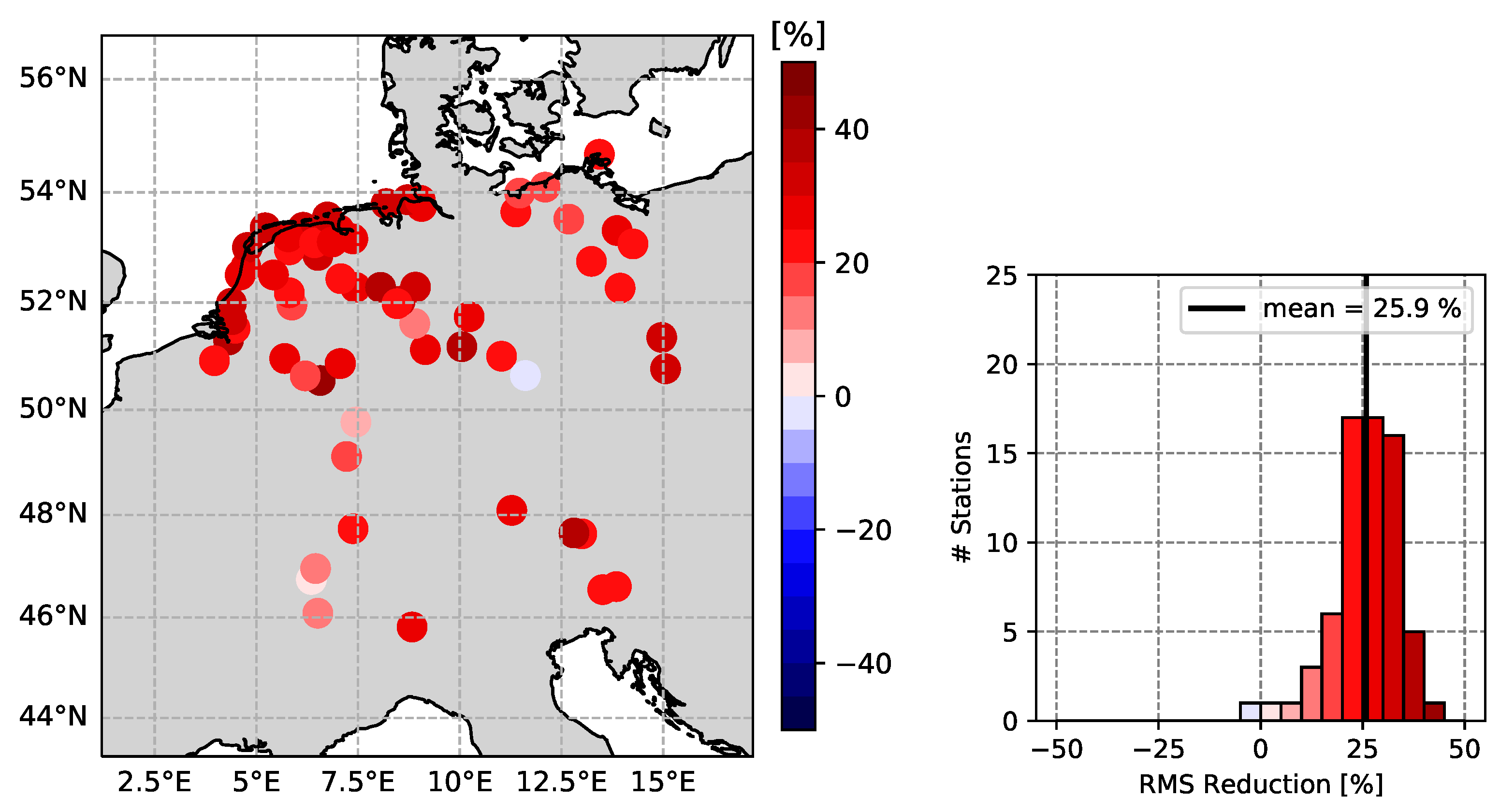
Figure 7 shows the spatial distribution and histogram of the achieved RMS reductions for all GNSS stations that were later used as test stations for the machine learning algorithm.
The average RMS reduction for these stations is 25.9%, with 98.5% of stations being positively reduced. The comparison to the state of the art in literature is not directly possible, as every study uses a different set of stations and loading models. Similar studies, which also focus on the area of Europe, are Bian [
5], achieving an average RMS reduction of 16–25%, and Springer et al. [
28], obtaining 20–30% with NTAL and NTOL and adding another 7% with HYDL.
3. Methodology
3.1. Temporal Convolutional Network
A Temporal Convolutional Network (TCN) is based on a sequence modeling problem, where a mapping function
maps an input sequence of length
T,
to an output
. The sequence modeling network tries to find the function
f that minimizes the expected loss
L between the true and predicted values:
[
29]. A popular method for the analysis of a long time series is the Long Short-Term Memory (LSTM) Network, which is based on a Recurrent Neural Network (RNN). In recent research, it was shown that TCN often outperforms LSTM as it is using both the advantages of an RNN, by processing high-level features, as well as the low-level feature computation from Convolutional Neural Networks (CNN) [
29,
30,
31,
32]. By using a radically different network architecture compared to RNNs, TCN is also overcoming any gradient vanishing problems, that can occur in deep networks with very long input sequences [
33]. The two main features of a TCN are:
- (1)
the network can take an input sequence of any length and return the same length as output by using a 1D fully convolutional architecture, and
- (2)
all convolutions are causal; therefore,
can only depend on
, and not any future inputs
[
29,
31]. In
Figure 8, the principle of dilated causal convolutions is depicted.
3.2. Implementation Details
After the previously described pre-processing steps (selection of stations and reduction by environmental surface loadings), all remaining datagaps are filled by linear interpolation over the whole time series. Overall, 342 stations are selected, from which 60% (206 stations) are used for training, 20% (68 stations) for validation, and 20% (68 stations) for testing. This ratio was adopted due to its wide use in literature and additional tests, that indicated better performance when increasing the number training stations. All stations were allocated randomly to the subsets.
Figure 9 shows the spatial distribution of the station categories. The input features per station are all meteorological parameters (temperature, precipitation, sea level pressure, humidity, and radiation), as well as location information (latitude, longitude, and height) in the form of constants over the whole time series. Both the input feature matrix and the target vector are scaled between 0 and 1 for the training of the network, and the results are scaled back to the original range again for analysis. Each training sample is represented by a sequence of F features, which can be represented as a matrix of size (FxT), with
F being the number of Features, and
T the time. During training, samples are grouped in batches of size B, leading to a 3-dimensional object of size (BxFxT), where B is the number of elements in the batch. In
Table 1 below, the utilized parameter values can be found, which were determined empirically. The TCN is implemented in Python, based on Bai et al. [
29], and a GitHub repository (
https://github.com/philipperemy/keras-tcn, accessed on 11 December 2020).
Figure 10 gives a schematic overview of the training, validation, and testing of the TCN. After dividing the dataset into its subsets, the TCN is trained on the meteorological parameters as input features, and the GNSS residuals as target features. In the validation, the meteorological parameters from the validation dataset are put through the TCN and then compared to the validation GNSS residuals to get a measure of how well the TCN is performing, as well as given information on the ability to generalize. When the model is sufficiently trained, the meteorological time series of the test dataset are used to model the GNSS time series
GNSSMOD. These are subtracted from the corresponding GNSS residuals from the test dataset, which results in the reduced GNSS time series
GNSSRED.
4. Results and Discussion
4.1. TCN Modeling and GNSS Reduction and Comparison to Physical Loading Model Reduction
This section shows the results of modeling the GNSS residuals through the TCN using time series of meteorological parameters as input parameters. The modeled signal is then subtracted from the GNSS time series and the RMS reduction is computed. These results are compared to the reduction of GNSS residuals by physical loading models from GFZ. The results of a TCN-modeled signal in the time and frequency domain is shown on the example station
MAR3 in
Figure 11. There is a clear seasonal pattern in the modeled signal, with the strongest peak in the annual amplitude. However, the semi-annual and other inter-annual amplitudes also follow the pattern of original GNSS residuals.
Figure 12 shows the RMS reduction rates for all stations when subtracting the TCN-modeled signal from the GNSS residuals. All stations are positively reduced, and the mean reduction rate is at 25.1%. The average reduction rate is slightly smaller than when using the physical models for reduction (see
Figure 7), but, overall, 36 out of 68 stations (52.9%) have a higher reduction rate when modeling the signal with meteorological parameters through a TCN. In
Figure 13, the differences in RMS reductions between the TCN and physical model reduction are depicted. A positive difference means that the TCN-modeled signal gave a higher reduction. The results demonstrate that it is possible to reproduce comparable reductions through a deep learning model using only meteorological parameters as input features. The physical models are, on the one hand, complex to compute, but, on the other hand, once they are computed, the complete dataset can be introduced into the GNSS residual computation at once and on all stations. The approach via a deep learning network works with minimally processed data, but the training of the network is time consuming and needs a lot of training data. In the evaluation of the trained model, not all stations can be reduced, only those that are dedicated test stations.
4.2. TCN Modeling Based on GNSS Residuals Reduced by Loading Models
The results of the direct subtraction of environmental loadings and of a meteorological-modeled time series from the GNSS residuals yield a similar level of RMS reduction. Therefore, in a second approach, the TCN model is trained on the GNSS residuals already reduced by environmental loadings. The idea is to increase the RMS reduction, by learning the potentially mis-modeled or leftover parts related to meteorological features. Once the model is trained, the correction signal is modeled for each test station and then subtracted from the reduced GNSS time series.
Figure 14 shows the results of the TCN-modeled time series, at
MAR3. Similar to the results of the previous section (
Figure 11), the seasonal patterns are very strong in the modeled signal. The annual peak is here even more distinct. The patterns of the underlying GNSS residuals are also different, as the environmental loadings were already subtracted. An interesting observation concerns the amplitude of the annual signal. Despite a smaller RMS variation overall, the annual peak is higher compared to the original GNSS residuals. This is due to a stronger annual signal in the environmental loading, mainly introduced by HYDL. HYDL has a clear annual pattern, which is, at most stations, not entirely in phase with the GNSS residuals. Phase differences between HYDL and GNSS have been quantified and discussed in several studies [
34,
35,
36]. The reasons found are diverse and mostly trace back to local phase-inhomogeneities of surface water and the absence of a model for groundwater storage, but no correction models are proposed. Only recently, Michel et al. [
37] made an attempt to model and correct for a misinterpretation of horizontal fluxes, which leads to an improvement of the phase advance over the GNSS seasonal signal. In our work, phase deviations are not corrected; therefore, the annual signal is inflated for some stations. These seasonal peaks get reduced by the TCN-modeled signal to a lower level than the original GNSS residuals. The different stages of reduced GNSS time series are shown in
Figure 15.
The additional RMS reduction of the GNSS residuals is computed, as well, and is depicted in
Figure 16. The achieved additional RMS reduction is, on average, 2.7%. Overall, the RMS of 84% of the stations could be further reduced.
In a final step, all reductions are applied to the GNSS residuals, and, again, the RMS reduction rate is computed and shown in
Figure 17. The average RMS reduction is now at 28.6%, with a maximum reduction of 44% at station
KALL. Only one station is negatively affected, meaning that the RMS of the variations in the height time series increased after all reductions.
5. Conclusions and Outlook
The aim of this work was to decrease the RMS of GNSS height residual time series by correcting them for environmental influences. First, the residuals were corrected for environmental surface loadings, which reduced the RMS of the time series, on average, by 25.9%. These results were compared to the RMS reduction, achieved by reducing the residuals by a time series modeled by a temporal convolutional neural network (TCN). The TCN was thereby trained on 206 stations to learn the relationship between meteorological parameters (temperature, precipitation, sea level pressure, humidity, and radiation) and the GNSS height residuals. The mean RMS reduction, achieved by reducing the GNSS residuals by the TCN-modeled signal, reached 25.1%. Although the mean RMS reduction through the TCN is slightly smaller, the majority of stations (52.9%) have a higher RMS reduction when using the signal modeled by the TCN. This suggests that the physical models can be recreated to great extend through a machine learning approach.
In a second experiment, the TCN was trained on the time series already reduced by environmental loading models. The mean additional RMS reduction of the residual time series was 2.7%, suggesting a relationship of the remaining residuals and meteorological features. Adding up both reductions, by environmental loading models and the TCN-modeled signal, the overall average RMS reduction was 28.6%, where 98.5% of the test stations were positively reduced, demonstrating the strong potential of applying machine learning models for GNSS time series modeling.
This study can be extended by using gridded meteorological data from numerical weather models to include more available GNSS stations. The current model could be improved by further hyperparameter tuning in an extensive grid search and complemented by a comparison to different machine learning algorithms. Furthermore, the approach could be extended by testing other study regions, and, in a following step, the derivation of global models could be evaluated.
Author Contributions
Conceptualization, P.R., R.H. and B.S.; methodology, P.R., R.H., S.D., J.D.W. and B.S.; software, P.R.; validation, P.R.; formal analysis, P.R., R.H. and B.S.; investigation, P.R., R.H. and B.S.; resources, P.R.; data curation, P.R.; writing—original draft preparation, P.R.; writing—review and editing, R.H., S.D., J.D.W. and B.S.; visualization, P.R.; supervision, R.H. and B.S. All authors have read and agreed to the published version of the manuscript.
Funding
This research received no external funding.
Institutional Review Board Statement
Not applicable.
Informed Consent Statement
Not applicable.
Data Availability Statement
The data presented in this study are available on request from the corresponding author.
Conflicts of Interest
The authors declare no conflict of interest.
References
- van Dam, T.M.; Blewitt, G.; Heflin, M.B. Atmospheric pressure loading effects on Global Positioning System coordinate determinations. J. Geophys. Res. Space Phys. 1994, 99, 23939–23950. [Google Scholar] [CrossRef]
- van Dam, T.M.; Wahr, J.; Chao, Y.; Leuliette, E. Predictions of crustal deformation and of geoid and sea-level variability caused by oceanic and atmospheric loading. Geophys. J. Int. 1997, 129, 507–517. [Google Scholar] [CrossRef]
- Dam, T.V.; Wahr, J.; Milly, P.C.D.; Shmakin, A.B.; Blewitt, G.; Lavallée, D.; Larson, K.M. Crustal displacements due to continental water loading. Geophys. Res. Lett. 2001, 28, 651–654. [Google Scholar] [CrossRef] [Green Version]
- Gegout, P.; Boy, J.P.; Hinderer, J.; Ferhat, G. Modeling and Observation of Loading Contribution to Time-Variable GPS Sites Positions. In Gravity, Geoid and Earth Observation; Mertikas, S.P., Ed.; Springer: Berlin/Heidelberg, Germany, 2010; pp. 651–659. [Google Scholar] [CrossRef]
- Bian, Y. Comparisons of GRACE and GLDAS derived hydrological loading and the impacts on the GPS time series in Europe. Acta Geodyn. Geomater. 2020, 17, 297–310. [Google Scholar] [CrossRef]
- Jiang, W.; Li, Z.; van Dam, T.; Ding, W. Comparative analysis of different environmental loading methods and their impacts on the GPS height time series. J. Geod. 2013, 87, 687–703. [Google Scholar] [CrossRef]
- Wu, S.; Nie, G.; Meng, X.; Liu, J.; He, Y.; Xue, C.; Li, H. Comparative Analysis of the Effect of the Loading Series from GFZ and EOST on Long-Term GPS Height Time Series. Remote Sens. 2020, 12, 2822. [Google Scholar] [CrossRef]
- Li, C.; Huang, S.; Chen, Q.; Dam, T.V.; Fok, H.S.; Zhao, Q.; Wu, W.; Wang, X. Quantitative Evaluation of Environmental Loading Induced Displacement Products for Correcting GNSS Time Series in CMONOC. Remote Sens. 2020, 12, 594. [Google Scholar] [CrossRef] [Green Version]
- Deng, L.; Chen, H.; Ma, A.; Chen, Q. Non-Tidal Mass Variations in the IGS Second Reprocessing Campaign: Interpretations and Noise Analysis from GRACE and Geophysical Models. Remote Sens. 2020, 12, 2477. [Google Scholar] [CrossRef]
- Karegar, M.A.; Dixon, T.H.; Kusche, J.; Chambers, D.P. A New Hybrid Method for Estimating Hydrologically Induced Vertical Deformation From GRACE and a Hydrological Model: An Example From Central North America. J. Adv. Model. Earth Syst. 2018, 10, 1196–1217. [Google Scholar] [CrossRef]
- Klos, A.; Karegar, M.A.; Kusche, J.; Springer, A. Quantifying Noise in Daily GPS Height Time Series: Harmonic Function Versus GRACE-Assimilating Modeling Approaches. IEEE Geosci. Remote Sens. Lett. 2021, 18, 627–631. [Google Scholar] [CrossRef]
- Mémin, A.; Boy, J.P.; Santamaría-Gómez, A. Correcting GPS measurements for non-tidal loading. GPS Solut. 2020, 24, 45. [Google Scholar] [CrossRef]
- Siemuri, A.; Kuusniemi, H.; Elmusrati, M.S.; Välisuo, P.; Shamsuzzoha, A. Machine Learning Utilization in GNSS—Use Cases, Challenges and Future Applications. In Proceedings of the 2021 International Conference on Localization and GNSS (ICL-GNSS), Tampere, Finland, 1–3 June 2021; pp. 1–6. [Google Scholar] [CrossRef]
- Benevides, P.; Catalao, J.; Miranda, P.M.A. On the inclusion of GPS precipitable water vapour in the nowcasting of rainfall. Nat. Hazards Earth Syst. Sci. 2015, 15, 2605–2616. [Google Scholar] [CrossRef] [Green Version]
- Benevides, P.; Catalão, J.; Nico, G.; Miranda, P.M.A. Evaluation of rainfall forecasts combining GNSS precipitable water vapor with ground and remote sensing meteorological variables in a neural network approach. In Remote Sensing of Clouds and the Atmosphere XXIII; International Society for Optics and Photonics: Berlin, Germany, 2018; Volume 10786, p. 1078607. [Google Scholar] [CrossRef]
- Li, H.; Wang, X.; Zhang, K.; Wu, S.; Xu, Y.; Liu, Y.; Qiu, C.; Zhang, J.; Fu, E.; Li, L. A neural network-based approach for the detection of heavy precipitation using GNSS observations and surface meteorological data. J. Atmosp. Sol.-Terr. Phys. 2021, 225, 105763. [Google Scholar] [CrossRef]
- Łoś, M.; Smolak, K.; Guerova, G.; Rohm, W. GNSS-Based Machine Learning Storm Nowcasting. Remote Sens. 2020, 12, 2536. [Google Scholar] [CrossRef]
- Selbesoglu, M.O. Prediction of tropospheric wet delay by an artificial neural network model based on meteorological and GNSS data. Eng. Sci. Technol. Int. J. 2020, 23, 967–972. [Google Scholar] [CrossRef]
- Li, L.; Xu, Y.; Yan, L.; Wang, S.; Liu, G.; Liu, F. A Regional NWP Tropospheric Delay Inversion Method Based on a General Regression Neural Network Model. Sensors 2020, 20, 3167. [Google Scholar] [CrossRef]
- Mohammed, J. Artificial neural network for predicting global sub-daily tropospheric wet delay. J. Atmosp. Sol.-Terr. Phys. 2021, 217, 105612. [Google Scholar] [CrossRef]
- Miotti, L.; Shehaj, E.; Geiger, A.; D’Aronco, S.; Wegner, J.D.; Moeller, G.; Rothacher, M. Tropospheric delays derived from ground meteorological parameters: Comparison between machine learning and empirical model approaches. In Proceedings of the 2020 European Navigation Conference (ENC), Dresden, Germany, 23–24 November 2020; pp. 1–10. [Google Scholar] [CrossRef]
- Mohammednour, A.B.; Özdemir, A.T. GNSS positioning accuracy improvement based on surface meteorological parameters using artificial neural networks. Int. J. Commun. Syst. 2020, 33, e4373. [Google Scholar] [CrossRef]
- Blewitt, G.; Hammond, W.C.; Kreemer, C. Harnessing the GPS Data Explosion for Interdisciplinary Science. Eos 2018, 99, 485. [Google Scholar] [CrossRef]
- Bos, M.S.; Fernandes, R.M.S.; Williams, S.D.P.; Bastos, L. Fast error analysis of continuous GNSS observations with missing data. J. Geod. 2013, 87, 351–360. [Google Scholar] [CrossRef] [Green Version]
- Dill, R.; Dobslaw, H. Numerical simulations of global-scale high-resolution hydrological crustal deformations. J. Geophys. Res. Solid Earth 2013, 118, 5008–5017. [Google Scholar] [CrossRef]
- Ruttner, P. Analysis and Prediction of Long Term GNSS Height Time Series and Environmental Loading Effects; ETH Zurich: Zurich, Switzerland, 2021. [Google Scholar] [CrossRef]
- Klein Tank, A.M.G.; Wijngaard, J.B.; Können, G.P.; Böhm, R.; Demarée, G.; Gocheva, A.; Mileta, M.; Pashiardis, S.; Hejkrlik, L.; Kern-Hansen, C.; et al. Daily dataset of 20th-century surface air temperature and precipitation series for the European Climate Assessment. Int. J. Climatol. 2002, 22, 1441–1453. [Google Scholar] [CrossRef]
- Springer, A.; Karegar, M.A.; Kusche, J.; Keune, J.; Kurtz, W.; Kollet, S. Evidence of daily hydrological loading in GPS time series over Europe. J. Geod. 2019, 93, 2145–2153. [Google Scholar] [CrossRef]
- Bai, S.; Kolter, J.Z.; Koltun, V. An Empirical Evaluation of Generic Convolutional and Recurrent Networks for Sequence Modeling. arXiv 2018, arXiv:1803.01271. [Google Scholar]
- Lea, C.; Flynn, M.D.; Vidal, R.; Reiter, A.; Hager, G.D. Temporal Convolutional Networks for Action Segmentation and Detection. In Proceedings of the 2017 IEEE Conference on Computer Vision and Pattern Recognition (CVPR), Honolulu, HI, USA, 21–26 July 2017; pp. 1003–1012. [Google Scholar] [CrossRef] [Green Version]
- Yan, J.; Mu, L.; Wang, L.; Ranjan, R.; Zomaya, A.Y. Temporal Convolutional Networks for the Advance Prediction of ENSO. Sci. Rep. 2020, 10, 8055. [Google Scholar] [CrossRef] [PubMed]
- Hewage, P.; Behera, A.; Trovati, M.; Pereira, E.; Ghahremani, M.; Palmieri, F.; Liu, Y. Temporal convolutional neural (TCN) network for an effective weather forecasting using time-series data from the local weather station. Soft Comput. 2020, 24, 16453–16482. [Google Scholar] [CrossRef] [Green Version]
- Li, R.; Chu, Z.; Jin, W.; Wang, Y.; Hu, X. Temporal Convolutional Network Based Regression Approach for Estimation of Remaining Useful Life. In Proceedings of the 2021 IEEE International Conference on Prognostics and Health Management (ICPHM), Detroit, MI, USA, 7–9 June 2021; pp. 1–10. [Google Scholar] [CrossRef]
- Xue, L.; Fu, Y.; Martens, H.R. Seasonal hydrological loading in the Great Lakes region detected by GNSS: A comparison with hydrological models. Geophys. J. Int. 2021, 226, 1174–1186. [Google Scholar] [CrossRef]
- Hsu, Y.J.; Fu, Y.; Bürgmann, R.; Hsu, S.Y.; Lin, C.C.; Tang, C.H.; Wu, Y.M. Assessing seasonal and interannual water storage variations in Taiwan using geodetic and hydrological data|Elsevier Enhanced Reader. Earth Planet. Sci. Lett. 2020, 550, 116532. [Google Scholar] [CrossRef]
- Materna, K.; Feng, L.; Lindsey, E.O.; Hill, E.M.; Ahsan, A.; Alam, A.K.M.K.; Oo, K.M.; Than, O.; Aung, T.; Khaing, S.N.; et al. GNSS characterization of hydrological loading in South and Southeast Asia. Geophys. J. Int. 2021, 224, 1742–1752. [Google Scholar] [CrossRef]
- Michel, A.; Santamaría-Gómez, A.; Boy, J.P.; Perosanz, F.; Loyer, S. Analysis of GNSS Displacements in Europe and Their Comparison with Hydrological Loading Models. Remote Sens. 2021, 13, 4523. [Google Scholar] [CrossRef]
Figure 1.
Distribution of selected GNSS stations over Europe. The size of the circles indicates the available time series length in years.
Figure 1.
Distribution of selected GNSS stations over Europe. The size of the circles indicates the available time series length in years.
Figure 2.
Environmental surface loadings at station MAR3. For visualization purposes, HYDL is shifted by +30 mm, NTOL by −15 mm, and the SUM (HYDL + NTAL + NTOL) by −30 mm.
Figure 2.
Environmental surface loadings at station MAR3. For visualization purposes, HYDL is shifted by +30 mm, NTOL by −15 mm, and the SUM (HYDL + NTAL + NTOL) by −30 mm.
Figure 3.
Time series of the meteorological parameters at the example station MAR3. TG = Temperature, RR = Precipitation, PP = Sea level pressure, HU = Humidity, QQ = Radiation.
Figure 3.
Time series of the meteorological parameters at the example station MAR3. TG = Temperature, RR = Precipitation, PP = Sea level pressure, HU = Humidity, QQ = Radiation.
Figure 4.
(Left) GNSS and meteorological station locations. (Right) GNSS station locations, colored by the distance to the corresponding meteorological station.
Figure 4.
(Left) GNSS and meteorological station locations. (Right) GNSS station locations, colored by the distance to the corresponding meteorological station.
Figure 5.
Workflow of GNSS data processing. The main input and output datasets are colored in green, processing steps are marked in orange, and the intermediate products are in colored in red.
Figure 5.
Workflow of GNSS data processing. The main input and output datasets are colored in green, processing steps are marked in orange, and the intermediate products are in colored in red.
Figure 6.
Processing steps of example station MAR3.
Figure 6.
Processing steps of example station MAR3.
Figure 7.
RMS reduction of GNSS height residuals after subtracting the sum of all environmental surface loadings.
Figure 7.
RMS reduction of GNSS height residuals after subtracting the sum of all environmental surface loadings.
Figure 8.
Example of a dilated causal convolution, with a filter size and dilation factors .
Figure 8.
Example of a dilated causal convolution, with a filter size and dilation factors .
Figure 9.
Categorization of GNSS stations into subgroups for training, validation, and testing.
Figure 9.
Categorization of GNSS stations into subgroups for training, validation, and testing.
Figure 10.
Flowchart of TCN training pipeline. The main input and output datasets are colored in green, processing steps are marked in orange, and the intermediate products are in colored in red and blue.
Figure 10.
Flowchart of TCN training pipeline. The main input and output datasets are colored in green, processing steps are marked in orange, and the intermediate products are in colored in red and blue.
Figure 11.
Example of TCN-modeled residuals at the example station MAR3. In blue are the GNSS residuals, and in orange are the TCN-modeled time series.
Figure 11.
Example of TCN-modeled residuals at the example station MAR3. In blue are the GNSS residuals, and in orange are the TCN-modeled time series.
Figure 12.
RMS reduction of GNSS height residuals after subtracting a TCN-modeled signal with meteorological parameters as input features.
Figure 12.
RMS reduction of GNSS height residuals after subtracting a TCN-modeled signal with meteorological parameters as input features.
Figure 13.
Difference in RMS reductions between the reduction rates of GNSS residuals when using the physical models from GFZ and a TCN-modeled signal from meteorological parameters.
Figure 13.
Difference in RMS reductions between the reduction rates of GNSS residuals when using the physical models from GFZ and a TCN-modeled signal from meteorological parameters.
Figure 14.
Example of resulting modeled residuals at the example station MAR3. In blue are the by environmental loadings reduced residuals, and in orange are the TCN-modeled time series.
Figure 14.
Example of resulting modeled residuals at the example station MAR3. In blue are the by environmental loadings reduced residuals, and in orange are the TCN-modeled time series.
Figure 15.
GNSS residuals at the different reduction stages. In blue are the original GNSS residuals, in orange are the time series after subtracting the environmental loading displacements, and the green residuals result after subtracting the TCN-modeled time series.
Figure 15.
GNSS residuals at the different reduction stages. In blue are the original GNSS residuals, in orange are the time series after subtracting the environmental loading displacements, and the green residuals result after subtracting the TCN-modeled time series.
Figure 16.
RMS reduction of reduced GNSS height residuals after subtracting a TCN-modeled signal with meteorological parameters as input features.
Figure 16.
RMS reduction of reduced GNSS height residuals after subtracting a TCN-modeled signal with meteorological parameters as input features.
Figure 17.
Total RMS reduction of GNSS height residuals after subtracting environmental surface loadings and the TCN-modeled signal.
Figure 17.
Total RMS reduction of GNSS height residuals after subtracting environmental surface loadings and the TCN-modeled signal.
Table 1.
Parameter values of the TCN architecture.
Table 1.
Parameter values of the TCN architecture.
| Parameter | Value(s) |
|---|
| batch size B | 2 |
| number of features F | 8 |
| sequence length (epochs) T | 7 |
| filter size k | 8 |
| dilations d | 1, 2, 4, 8, 16, 32, 64, 128, 256 |
| number of filters | 24 |
| Publisher’s Note: MDPI stays neutral with regard to jurisdictional claims in published maps and institutional affiliations. |
© 2021 by the authors. Licensee MDPI, Basel, Switzerland. This article is an open access article distributed under the terms and conditions of the Creative Commons Attribution (CC BY) license (https://creativecommons.org/licenses/by/4.0/).


