1. Introduction
In recent years, smart cities have been recognized as a promising research hotspot around the world [
1,
2,
3]. The analysis and utilization of big data are key factors to realize smart cities. More specifically, exploring the spatio-temporal patterns of human mobility based on multi-source big data plays an important role in analyzing the formation of social-economic phenomena in smart cities. However, our acquired knowledge is still very limited for smart cities. For instance, smart cities face some challenging problems, including mobility pattern analysis, data management, data islands, etc. In this study, we mainly focus on the first of these challenges.
Nowadays, the analysis and exploration of human mobility patterns have been a hot research field related to transportation management and urban planning, benefiting from the ubiquitous intelligent traffic detectors. With the advances in data-acquisition technology from traditional surveys to cell phones, wireless network traces, and GPS-equipped taxis, researchers are able to better understand human mobility patterns. However, these currently available data are slightly inadequate in terms of data scale, spatio-temporal coverage, temporal frequency, and positioning accuracy [
4]. Consequently, it is difficult to use these data to explore human mobility deeply and accurately. Therefore, alternative data sources are needed.
Recently, as location-sensing devices and apps have become more mature and prevalent, online car-hailing platforms (e.g., Uber, Lyft, and Didi Chuxing) have played an increasingly important role in human daily mobility. As an emerging travel mode, they generate a large amount of accurate location data, which contain rich and detailed information about the travel patterns of individuals and traffic conditions, etc. More specifically, online car-hailing data are characterized by large-scale, high-resolution and high-quality, which compensates for the shortcomings of the data mentioned above. Therefore, this brings about new opportunities and challenges to further understand human travel behavior and intra-urban mobility. With these trajectory data, researchers have achieved fruitful results in many aspects, such as human mobility [
5,
6,
7,
8], travel behavior prediction [
9], traffic emissions [
10,
11], and demand and supply patterns [
12]. The related work is detailed in the following section.
Previous studies have proposed a number of human mobility patterns, such as the Lévy flight model, power-law, exponential, lognormal, Gamma, Weibull, Pareto and Rayleigh. At first, the long tail distributions are mainly applied to describe travel time. Specifically, Jiang et al., Rhee et al., and Zheng et al. observed that the statistical patterns of human mobility from GPS traces are similar to the Lévy flight model [
13,
14,
15]. More specifically, a power law distribution (or with exponential cutoff) can be used to approximate the displacement distribution of human trajectories collected from mobile phones [
4,
16], GPS traces [
8,
17,
18], and online location-based social networks [
19]. However, Liang et al. reported that daily travel time tends to be an exponential distribution rather than power laws [
20]. Similar results were also found in Kang et al., Jiang et al., and Yan et al. [
21,
22,
23,
24]. Cai et al. found that trip displacement of short trips could be best fitted with power-law distribution, while long trips follow exponential decay [
18]. Csáji et al. and Zhang et al. found that the exponential distribution is not appropriate for travel distances, while the lognormal distribution provide reasonable fits [
5,
25]. Tang et al. found that travel speed distribution has obviously different patterns compared with travel distance and travel time, and can be well fitted with lognormal distribution [
8].
Furthermore, some existing studies found that there is no stable pattern for human mobility. Zheng et al. found that a fusion function based on exponential power law and a truncated Pareto distribution represents travel time distribution best [
15]. Bazzani et al. studied the GPS data of private cars in Florence, Italy and found that the single-trip length follows an exponential behavior in the short distance scale but favors a power law distribution for trips longer than 30 km [
26]. Plötz et al. used Weibull, Gamma, and lognormal distributions to fit individual daily driving distances, and found that Weibull and lognormal most often perform better than Gamma, and the Weibull distribution fits most data but not all [
27]. Kou and Cai analyzed the distributions of travel distance and travel time, and found that both of them follow a lognormal distribution in larger bike sharing systems, while the distribution for smaller systems varies among Weibull, Gamma, and lognormal [
28].
To the best of our knowledge, the above studies proposed a number of spatio-temporal human mobility patterns. Although these findings mentioned above can provide a good foundation and a beneficial reference for understanding human mobility patterns, they are mostly based on small-scale, low-precision and low-frequency data, which is insufficient to analyze the human mobility deeply and accurately. Moreover, the mobility patterns may be different based on various research data. However, based on massive trajectory data collected from Didi Chuxing in Xi’an, China, will the mobility patterns be different from those reported in the existing literature? If so, what are the new mobility patterns and how will they vary? This remains to be further explored. Therefore, this study is indispensable and can gain valuable insight into human mobility patterns, so as to address some of the challenges in smart cities.
To address these questions, this paper adopts a two-month dataset collected from about 18,000 online car-hails to analyze intra-urban travel patterns. Specifically, three mobility metrics, namely travel distance, travel time, and travel speed, are modeled with different distributions at different time granularities (e.g., daily, hourly). Based on the fitting distributions of mobility metrics, six key points, namely lower limit, first quartile (Q1), median (Q2), third quartile (Q3), interior upper limit, and extreme upper limit, are calculated and adopted to present the characteristics of daily and hourly mobility patterns.
The remainder of this paper is organized as follows.
Section 2 briefly introduces the study area, the dataset of online car-hailing, and carries out a basic analysis.
Section 3 describes the trip metrics, and presents the fitting results.
Section 4 reports the analysis and discussion of temporal travel patterns. Additionally,
Section 5 provides conclusions and recommendations for further research.
2. Data Collection and Basic Analysis
2.1. Study Area
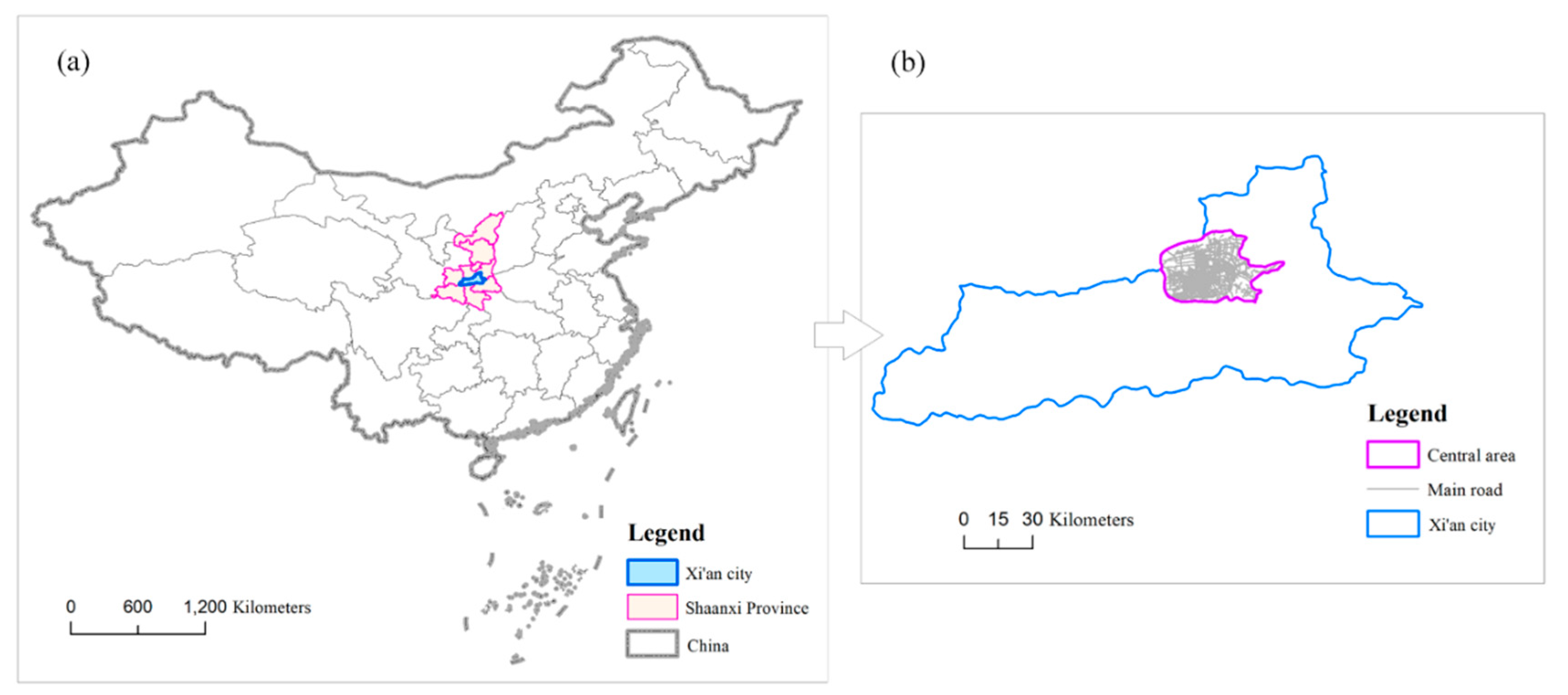
The research area of this paper is the central urban area of Xi’an, the capital city of Shanxi Province, China, as shown in
Figure 1a. This city has a permanent population of more than 10 million. In 2020, the city’s GDP exceeded 1 trillion yuan, with the fastest growth rate among the top 30. Xi’an is the most important city in Northwest China, with an urbanization rate 74.61%. The spatial location of Xi’an is shown in
Figure 1. Xi’an has developed into an influential international city. The prosperous socioeconomic status of Xi’an makes it a good choice for analysis of human mobility patterns in China.
As shown in
Figure 1b, the central area of Xi’an, China includes the districts of Xincheng, Beilin, Lianhu, Yanta, Weiyang, and Baqiao. These six districts are the most prosperous and oldest districts in Xi’an, where online car-hailing trajectory data are mainly distributed. Therefore, it is appropriate to choose Xi’an, China as the study area.
2.2. Data Description
The adopted trajectory data were generated by about 18,000 online car-hails in Xi’an, China, from 1 October 2016 to 30 November 2016. Each trajectory is a sequence of GPS sampling points with five fields, namely an anonymized vehicle ID (i.e., driver ID), an anonymized order ID (i.e., trip ID), a timestamp, longitude and latitude. These GPS sampling points are typically recorded every 2–4 s, which are at an unprecedented spatio-temporal resolution, thus providing a rich source of data that can be analyzed and directly mapped to human mobility patterns.
Let denote the trajectory of the trip of vehicle , where is the point of the sequence (). denotes the location and the timestamp, respectively. Given a trajectory, . For a vehicle, the origin and destination (OD) locations are the first and last sampling points of a trip. It makes sense to define and . Hence, each OD trip can be simplified to be a vector from to .
A road network consists of a set of nodes, directed links, and allowed movements. Each node is a geographical location representing a network intersection, which can be either signalized or non-signalized. A link is defined as the road section from its tail node to head node. The relative position denotes the ratio of a sampling point relative to the link tail node, which ranges . For example, the values 0, 0.5, and 1 of the relative position represent the beginning, middle and end of a link, respectively.
2.3. Data Precessing
In the existing studies, travel displacement and travel time are important mobility metrics, which can be obtained directly based on the trip’s OD. As another important mobility metric, travel distance can only be calculated after map matching (MM) and the path inference algorithm [
29]. Moreover, data cleaning is an essential task, because not all trips are suitable for this study. Considering travel costs, few passengers travel by online car-hailing when travel time and distance are very short or long [
3,
9]. In addition, the average travel speed should be within a reasonable range. Too low speed (e.g., less than 5 km/h) is beyond the traveler’s psychological tolerance range, while too high speed (e.g., more than 80 km/h) is not in line with the design requirements of urban roads. Therefore, the following conditions led to the exclusion of trip records from the study data: (1) travel distance between origin and destination less than 300 m; (2) travel time less than 1 min or longer than 2 h; (3) average travel speed below 5 km/h or in excess of 80 km/h [
6].
In terms of the trips over the course of two months, 6,203,848 trips were obtained from 6,584,397 original trips after data cleaning, which means that about 6% of the trips were filtered out, as shown in
Figure 2a. Daily valid orders fluctuate between 68,967 (the blue star, 17 October 2016) and 123,642 (the green star, 5 November 2016), with an average of 102,457. The average order availability is 94.22%, which fluctuates between 93.21% and 94.85%. More commonly, the study period is discretized into 1464 (24 h*61 days) 1 h intervals for further analysis of residents’ hourly trips. The hourly trip quantity ranges from 192 to 8636, as shown in
Figure 2b. Overall, the number of trips during the day is much higher than those at night, which is in line with human mobility. After all, human mobility during the day is more active and important. In addition, the number of trips during the period 00:00–7:00 may be less than 2000, but is sufficient for distribution fitting.
4. Temporal Analysis and Discussion of Travel Patterns
In this section, based on the above fitting results of trip metrics, we firstly analyze the distributions of daily trip metrics. Secondly, the distributions of hourly trip metrics, including travel distance, travel time and travel speed, are discussed in detail, respectively.
4.1. Analysis of Daily Trip Metrics
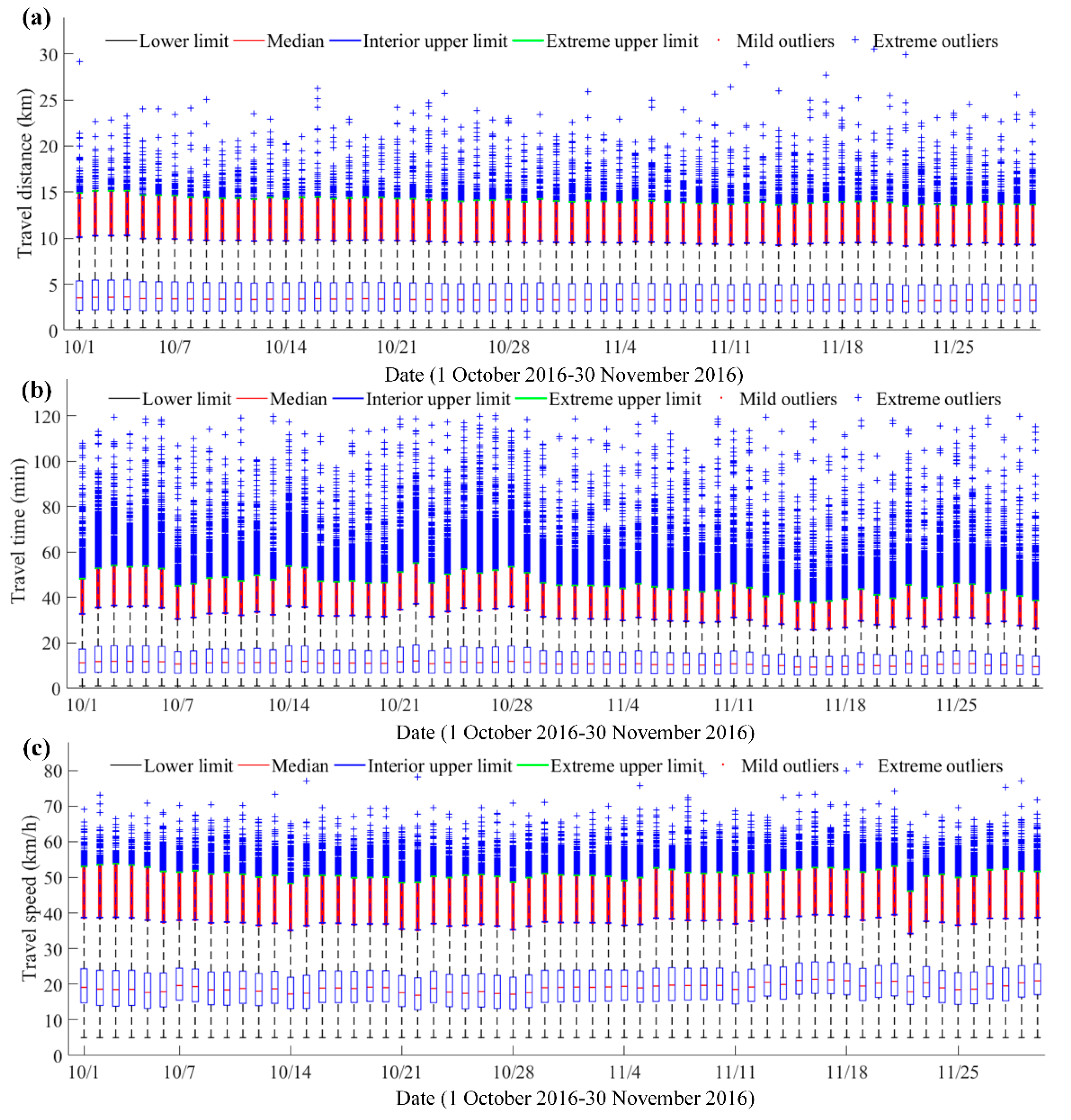
To understand the temporal travel patterns of daily trip metrics, the boxplot (also referred to as the box-whisker plot) is adopted to present the characteristics of daily distributions. The boxplot provides a simple way to summarize a dataset with five points (here extended to six points), including the lower limit, first quartile (Q1), median (Q2), third quartile (Q3), interior upper limit, and extreme upper limit. The trip data outside the interior upper limit are all outliers, where the outliers between the interior upper limit and extreme upper limit are mild outliers (as shown in the red dots in
Figure 4), and those outside the extreme upper limit are extreme outliers (as shown in the blue plus signs in
Figure 4).
Figure 4 shows the distribution shape, skewness, tail weight, and the outliers. The more the median deviates from the center position of the upper and lower quartiles, the stronger the distribution’s skewness. The outliers are concentrated on the larger side, which means the distribution is right-skewed. The percentages of these outliers are shown in
Table 2.
In
Figure 4a, the statistic characteristics of daily travel distance are similar with a small fluctuation. The daily distance metrics have an interquartile range (IQR) of 2.09–5.10 km, with a median of 3.36 km for travel distance (
Figure 4 and
Table 2). Overall, 97.84% (1–2.15%–0.01%) of travel distance data are for trips less than 9.61 km in length. However, some extreme outliers greater than 14.13 km appear in distance data, only accounting for 0.01%. In the travel distance data, 2.15% are mild outliers, varying between 9.61 and 14.13 km. Moreover, most residents travel by online car-hailing within 10 km, while for trips over 9.61 km, only 2.16% of people travel by online car-hailing, probably because of the high travel cost.
In
Figure 4b, it can be seen that the statistics of daily travel times fluctuate to a certain extent, and the travel time data, except for the National Day holiday, seem to indicate a weekly routine. From the second week to the seventh week (10 October 2016–27 November 2016), statistics for travel times on Friday and Saturday appear to be higher than other days of the week, which requires further analysis. Overall, 50% of travel time data fluctuate between 6.59 and 16.52 min, with a median of 10.81 min. Mild outliers between 31.41 and 46.30 min only account for 2.74% of the data, while the percentage of extreme outliers higher than 46.30 min is 0.49%. Meanwhile, 96.77% (1–2.74%–0.49%) of travel time data are for trips less than 31.41 min long, which indicates that most residents tend to use online car-hailing for short-term trips. Only 3.23% (2.74% + 0.49%) of residents prefer online car-hailing for long trips, indicating that only a minority do not consider the economic cost, or encounter congested road conditions. In addition, 99% of the travel time data are distributed within 48 min (40% of the travel time interval), while extreme outliers occupy more than 60% of the travel time interval. These phenomena show the value of boxplots in identifying extreme data.
Moreover, a weekly routine of travel time distributions can also be found in travel speed distribution, as shown in
Figure 4c. Statistics for travel speeds on Friday and Saturday seem to be lower than for other days of the week. Overall, 50% of travel speed data fluctuate between 14.94 and 23.97 km/h, with a median of 19.06 km/h. Vertically, 97.22% (1–2.59%–0.19%) of travel speed data are for trips with speeds below 37.50 km/h, accounting for half of the area in
Figure 4c. However, outliers (less than 3%) occupy the remaining half of the area, while the extreme outliers (0.19%) greater than 51.04 km/h account for more than 50%. In addition, it should be noted that travel speed on 22 November 2016 is significantly lower than other days, which may be due to the impact of abnormal weather. Based on the historical weather data, the only snowfall in the two months occurred on 22 November 2016.
Based on the above statistical analysis, we were able to gain a general understanding of the residents’ daily travel pattern, but the characteristics of hourly trip data need to be further analyzed in detail. Meanwhile, due to the extremely low resistance of mean and variance and susceptible to outliers, they may be not suitable for analyzing the daily and hourly trip data. The distribution characteristics of each hourly trip metric are analyzed in the following sections.
4.2. Analysis of Hourly Travel Distance Distribution
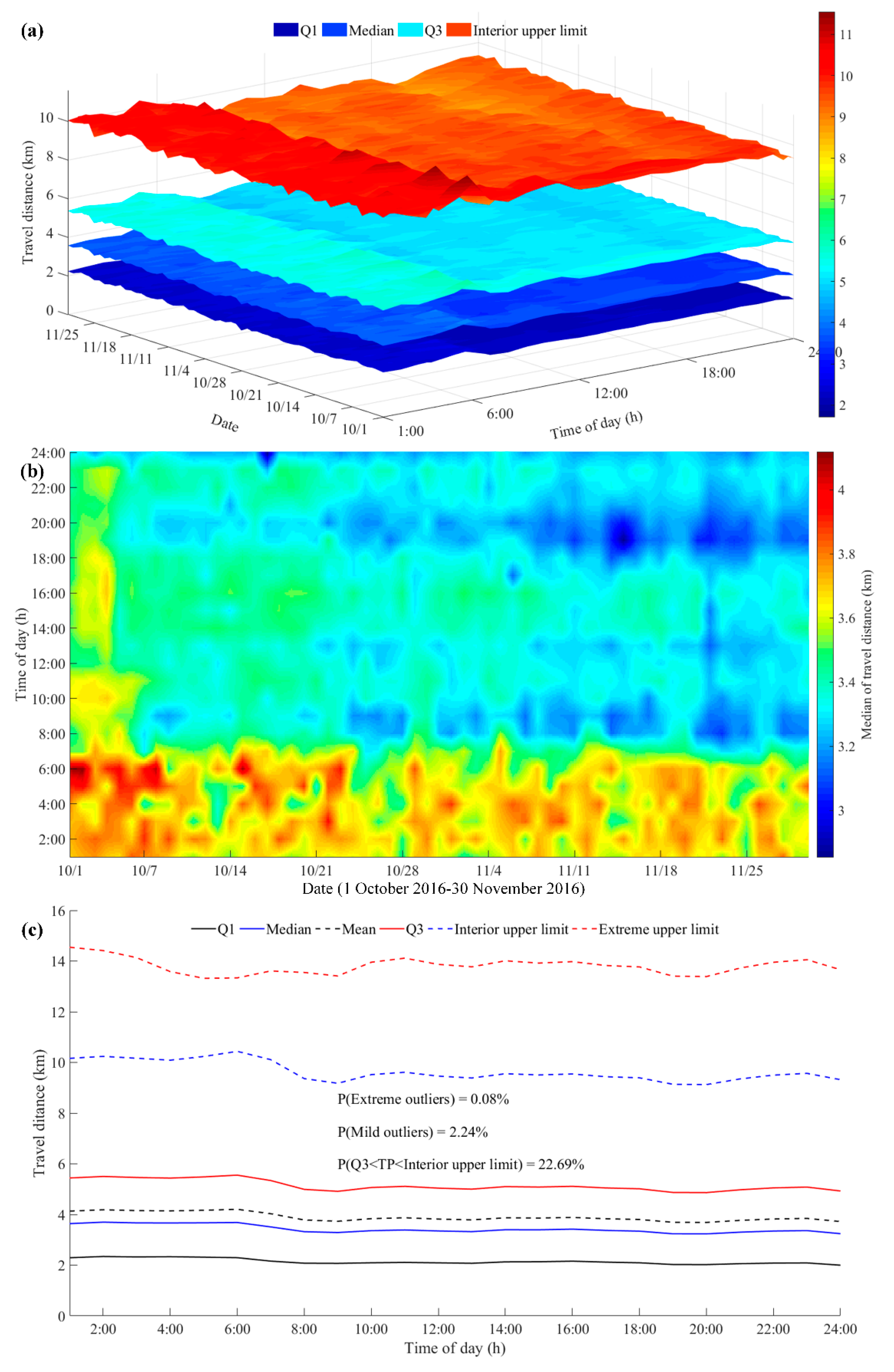
The distribution of hourly travel distance statistics is shown in
Figure 5a, from which the hourly and daily travel patterns can be found. Looking vertically from bottom to top, four statistical values (i.e., the first quartile, the median, the third quartile, and the interior upper limit) are displayed, and the statistics are represented by different colors. Meanwhile, it can also be found that the difference between statistical values gradually increases, from which we can roughly understand the shape and tail weight of hourly distance distribution. For all the hourly statistics, the medians deviate from the center of the upper and lower quartiles (Q1 and Q3) and are closer to the lower quartiles, indicating that the distribution has a strong skewness. Moreover, the large difference between Q3 and interior upper limit indicates that the long tail is distributed to the right, and it is more likely to have large outliers.
Horizontally, by observing the hourly and daily distributions in
Figure 5a,b, residents seem to travel with a certain regularity. First, hourly travel distances on different days have similar trends. For example, hourly travel distances from 0:00 to 7:00 are significantly higher than those in the remaining periods. This may be because public transportation is suspended at night, and residents have to choose online car-hailing. As another example, travel distances for the period 18:00–20:00 are smaller than those of other time periods, which suggests that people are more likely to take online car-hailing for short trips after work. Second, travel distances during the National Day holiday are higher than that on non-holidays, as shown in
Figure 5b. People usually travel much further on holidays than weekdays, which implies that people prefer to go for an outing or other social activities rather than work on weekends. Third, during the non-holidays, there appears to be a weekly pattern in the daily distance distribution. For example, in the morning (7:00–11:00), travel distances on weekends are higher than those on weekdays. The same pattern also exists in the afternoon (13:00–18:00).
Moreover, travel distances in October are higher than those in November, which may be caused by National Day holiday and rainfall. In general, residents often change their travel mode on rainy days, such as switching short trips by bike or on foot to taxis or online car-hailing. From the perspective of each hour, travel distances in the working period (10:00–12:00, 14:00–18:00) are significantly higher than that of other periods between 8:00 and 20:00.
Figure 5c shows the average hourly travel distance statistics for all 61 days. Based on the hourly statistics, the obvious positive skewness and long tail can be found. Half of the residents travel between 2.15 and 5.14 km, with a median of 3.43 km. In addition, 22.69% of residents travel further, but not more than 9.61 km. However, only 2.24% of residents travel further, reaching 13.80 km, which are accepted as mild outliers. Those who travel further, regardless of travel costs, account for just 0.08%. Thus, mild outliers and extreme outliers can be distinguished well, which may reflect the travel patterns of the minority.
To sum up, hourly travel distance can reflect human travel patterns more clearly and accurately. We note that more than 97% of trips are within 10 km in all the studied datasets, and 75% of trips are about 5 km long. This is fairly consistent with our daily experience. Mainly attributed to travel cost, individuals seldom use online car-hailing for long distance trips. People usually prefer the subway and other public transportation systems for longer-distance travel. However, long-distance trips using online car-hailing do happen for many reasons, such as rushing to catch flights or trains, or returning from airports or train stations after an exhausting trip, especially when carrying large or heavy luggage.
4.3. Analysis of Hourly Travel Time Distribution
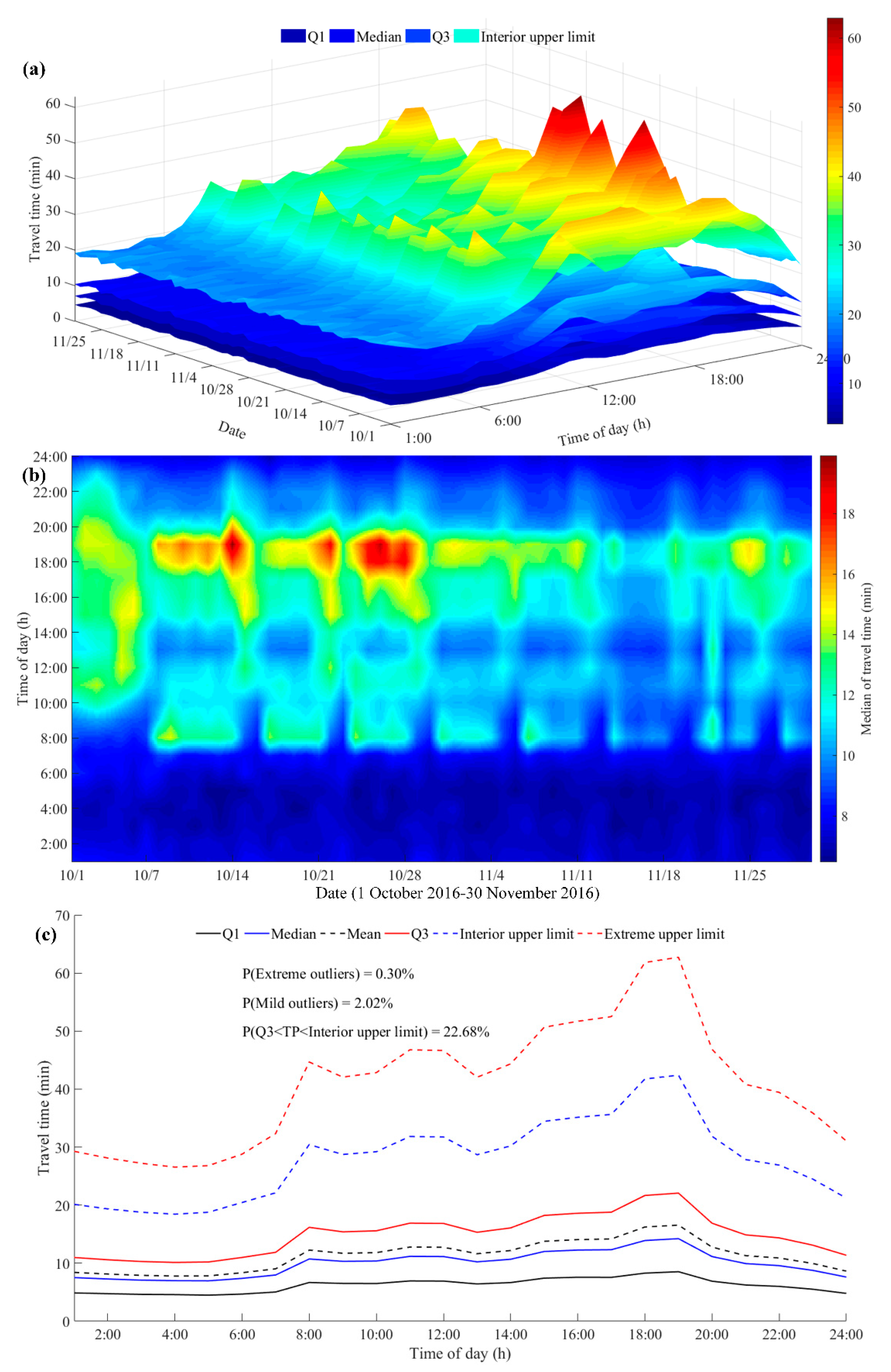
Travel time is another fundamental variable that explores travel patterns. In
Figure 6, we can find a few typical travel patterns. First of all, hourly travel times are mainly distributed in the left side of the distribution and are concentrated in a very narrow time interval. The hourly travel times have an IQR of 5.05 min–11.70 min, with a median of 7.91 min for the period 21:00–7:00 and an IQR of 7.14–17.58 min with a median of 11.58 min for the period 7:00–21:00. Nevertheless, for trips within 10 min, individuals are most likely to choose online car-hailing. Overall, 22.68% of travel times fall within the interior limit with an interval length of 10 min at night and 15 min during the day, which is 50% higher than the corresponding IQR. The outliers of travel time data account for 2.32%, indicating a few residents use online car-hailing for long trips.
Secondly, the morning and evening peaks can be clearly found in daily travel times and the median distribution of hourly travel times. Moreover, the evening peak is significantly higher than the morning peak, as shown in
Figure 6a,b. There is also an occasional peak during the period 10:00–12:00, followed by a two-hour trough. In addition, travel time during the day is significantly higher than that at night, which is consistent with our daily experience.
Thirdly, the National Day holiday presents some different travel patterns. Travel times gradually increase from 9:00 and continue until 22:00, during which there are no obvious peaks and troughs. On the one hand, this suggests that people can travel more freely, rather than during rush hours on weekdays. On the other hand, people can more leisurely choose when to start or end the activities, because there is no concern about work or study.
Finally, an obvious weekly pattern can be found in
Figure 6a,b. Most weekday trips start at 7:00, while people usually travel at around 10:00 on weekends. Moreover, similarly to holidays, travel times in the morning and evening rush hours are much lower than those on weekdays, or there are even no rush hours. Furthermore, several excessively high evening peaks in October show the potential impact of rainfall on travel.
4.4. Analysis of Hourly Travel Speed Distribution
This study also takes into consideration the relationship between travel distance and travel time, which implies the level of urban traffic conditions more deeply. Comparing
Figure 6 and
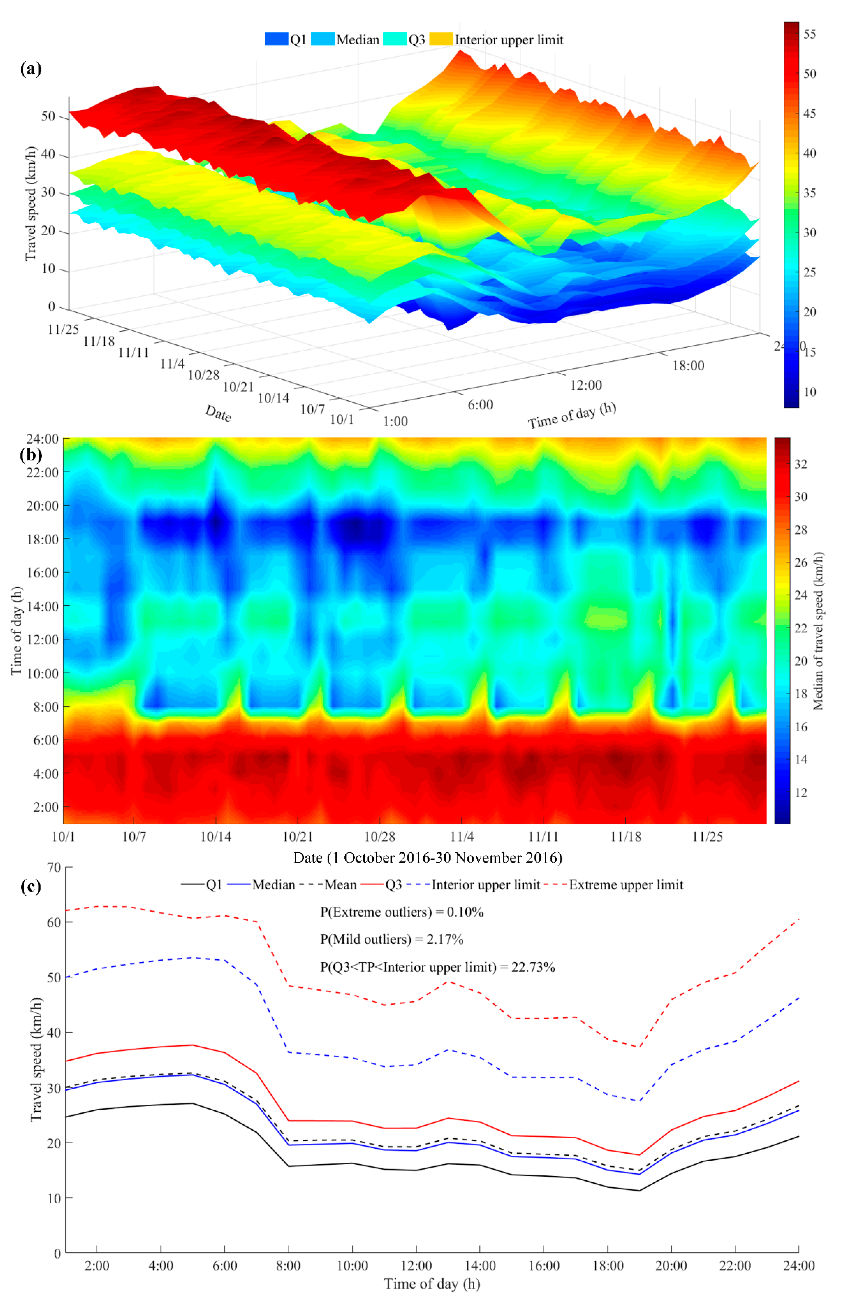
Figure 7, we can find that hourly travel time is inversely proportional to travel speed, but travel speed can more directly reflect urban traffic conditions. The median of hourly travel speed is very close to the midpoint of the IQR in
Figure 7a. Furthermore, the median and mean almost coincide, as shown by the solid blue line and the black dotted line in
Figure 7c. This indicates a decrease in the skewness of hourly speed distribution. Meanwhile, after converting travel time to travel speed, the average skewness and kurtosis decrease from 1.4952 and 8.9546 to 0.6945 and 4.3186, respectively, which further demonstrates that hourly speed distribution is similar to normal distribution.
In addition, the daily evening rush hour during non-holidays starts at 17:00 and lasts until 19:00, as shown in
Figure 7a,b. Then, the traffic condition eases and travel speed gradually increases until it reaches its highest value before dawn. This is in line with the law of human activities. As the night spreads, individuals will finish their activities and go home to rest, so the traffic condition is improved. When the morning comes, travel speed gradually decreases with human activity recovery, and then increases slightly at noon. In the afternoon, the traffic conditions are relatively stable and deteriorate at 17:00. Based on the above analysis, 6:00 can replace 24:00 as the new boundary for future analysis of human mobility patterns. With the prosperous development of society and the economy, human activities are more abundant and frequent. These activities usually last until night to early morning, especially on weekends and holidays.
Moreover, the weekly routine in hourly travel times also exists in the hourly travel speeds, as shown in
Figure 7b. In the morning, travel patterns on holidays and weekends are markedly different from those on weekdays. Most personal trips are postponed from 7:00 to 10:00. As can be seen from
Figure 7b, travel speed in October is lower than that in November, which may be caused by National Day holiday and rainfall. According to statistics, there are 14 days and 10 nights in October with rain, while there are only 3 days and 4 nights in November with rain or snow. In addition,
Figure 7b shows the impact of snowfall on traffic conditions in more detail. Travel speed on 22 November 2016 is significantly lower than other days.
Figure 7c shows the average hourly travel speed statistics for all 61 days. The hourly travel speeds have an IQR of 15.88–23.88 km/h, with a median of 19.63 km/h for the period 7:00–24:00, while these statistics for the period 00:00–7:00 are about 60% higher, namely 26.05 km/h, 36.52 km/h and 31.13 km/h, respectively. In addition, 22.73% of travel speeds fall between the upper quartile and the interior upper limit, with a mean interval length of 12.93 km/h, which is 50% greater than that of the corresponding IQR (8.62 km/h). The mild outliers of travel speed data account for 2.17%, indicating that a few lucky residents travel at high speeds. Moreover, the extreme outliers (0.10%) mean fewer residents travel at higher speeds.
5. Conclusions
In this paper, we use the trajectory data collected from Didi Chuxing in Xi’an, China to explore the temporal characterizations of intra-urban human travel patterns. Specifically, by analyzing distributions of three mobility metrics (i.e., travel distance, travel time, and travel speed), this study reveals that the trajectory data of online car-hailing can provide useful insights into residents’ mobility patterns. The main contributions of this paper are summarized as follows.
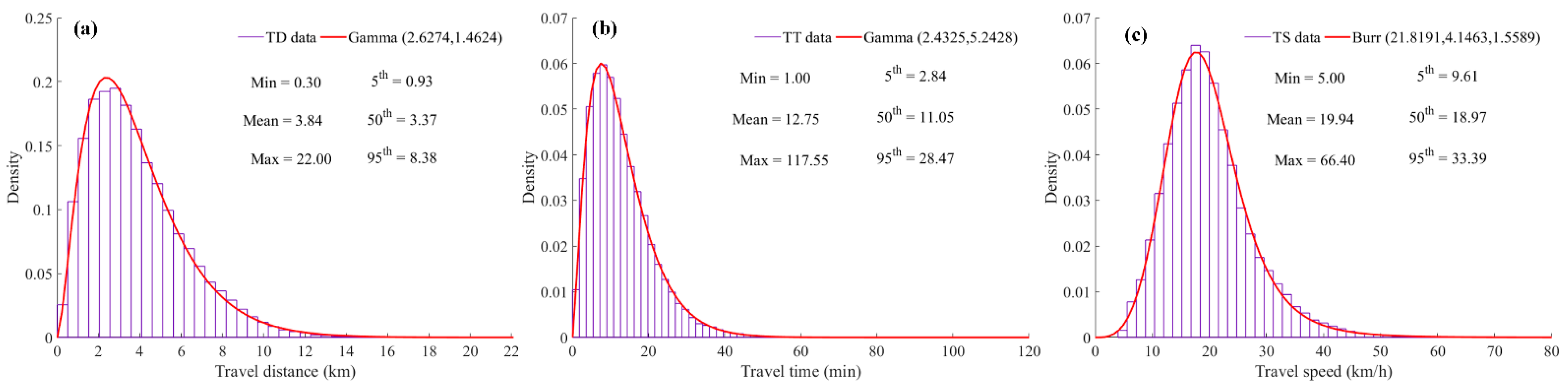
Firstly, the mobility patterns are different from statistical characteristics found in existing studies. Uncertain distribution types exist in the daily and hourly data, while the dominant distribution exists in each mobility metric. To be specific, the daily and hourly travel distance and travel time have a similar distribution, and can be approximated by Gamma distribution. However, travel speed distribution is quite different and more complicated, which tends to be Burr distribution.
Secondly, the statistical characteristics of the daily travel distance are similar, with a small fluctuation. The daily travel distance has an interquartile range (IQR) of 2.09–5.10 km, with a median of 3.36 km. About 98% of the travel distance data are for trips less than 10 km. In addition, for daily travel time and speed, the statistics fluctuate to a certain extent, and seem to be a weekly routine. More specifically, 50% of the travel time data fluctuate between 6.59 and 16.52 min, with a median value of 10.81 min, and about 97% of residents travel less than 30 min. Moreover, 50% of travel speed data represent speeds lower than 19 km/h, and only 25% of residents travel faster than 24 km/h.
Thirdly, a weekly pattern is more obvious in hourly mobility metrics, especially travel time and travel speed. Meanwhile, the diurnal statistics of hourly travel distance and travel speed are significantly smaller than those of other periods, while the opposite is true for travel time. In addition, the National Day holiday presents some different travel patterns. Travel times gradually increase from 9:00 and continue until 22:00, during which there are no obvious peaks and troughs. These results provide empirical evidence supporting the common regularity of intra-urban human mobility. Finally, rainfall and snowfall have a potential impact on residents’ travel patterns. Since October has more rainy days than November, travel distance and travel time distributions in October are higher than those in November, while the opposite is true for travel speed. In general, residents often change their travel mode on rainy days, such as switching short trips by bike or on foot to taxis or online car-hailing. Furthermore, several excessively high evening peaks in hourly travel time distributions also indicate the impact of rainfall on traffic conditions. In addition, the travel speed on 22 November 2016 is significantly lower than other days, indicating the impact of snowfall on traffic conditions.
Nevertheless, there are also several limitations in the current work, deserving further study. First, the adopted data are slightly outdated. With the acquisition of the fresh data (August 2020) in Shenzhen, China, we can update the data in the following research. Second, this study only analyzes temporal mobility patterns, ignoring spatial human mobility patterns. Additional research is needed to identify the spatio-temporal mobility patterns. Third, potential travel purpose analysis (i.e., going to work, going to dinner, recreational activities, hospital visits, shopping) is needed, which may help to express more interesting findings. Last but not least, human mobility patterns with respect to weather conditions, holidays, weekdays and weekends need further research.


