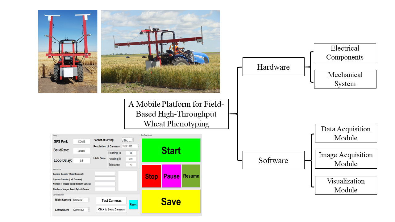
Development of a Mobile Platform for Field-Based High-Throughput Wheat Phenotyping

Abstract

Designing and implementing an affordable High-Throughput Phenotyping Platform (HTPP) for monitoring crops’ features in different stages of their growth can provide valuable information for crop-breeders to study possible correlation between genotypes and phenotypes. Conducting automatic field measurements can improve crop productions. In this research, we have focused on development of a mechatronic system, hardware and software, for a mobile, field-based HTPP for autonomous crop monitoring for wheat field. The system can measure canopy’s height, temperature, and vegetation indices and is able to take high quality photos of crops. The system includes. developed software for data and image acquisition. The main contribution of this study is autonomous, reliable, and fast data collection for wheat and similar crops.

1. Introduction

By continuous growth of population around the world, humanity’s needs for food resources increase, which leads to need for optimizing crop production. More than 820 million people in the world were suffering hunger in 2018 [1]. Moreover, there is a prediction that humanity’s demand for food and resources will double by 2050 within a 40-year period [2]. Analyzing genetic features of a plant is a necessary practice in agriculture related research to make an interaction between crop breeders and experts who use phenotyping to gather features of plants. However, phenotyping needs to be more advanced to provide more information. Measuring characteristics, such as plant’s height, temperature, and greenness, and having high quality pictures for image processing are challenging and time consuming.

The importance of plant phenotyping has been discussed in [3,4]. Phenoscope is a High-Throughput Phenotyping Platform (HTPP) for indoor cases [5]. In [6] a high-throughput non-destructive plant phenotyping platform, which has light curtain and spectral reflectance sensor, is proposed. Phenobot 1.0 is another ground-based platform that is designed for tall and densely planted crop species [7]. This field-based platform is auto-steered and self-propelled and is equipped with RGB (Red-Green-Blue) cameras that are positioned horizontally and vertically. Another platform is PhenoTrac4, equipped with ultrasonic sensors and infrared thermometer and able to measure height and temperature of crops [8].

In [9], a field-based platform is proposed that has several sensors, which are infrared thermometers, laser and ultrasonic sensors, Crop Circle, and Green Seeker sensors. Moreover, they [9] used two RTK (real-time base station correlation) GPS systems, while in our research, we managed to use just one RTX (real-time satellite corrections) GPS with accurate results. Another multi-sensor HTPP is proposed in [10]. The utilized NDVI sensors are passive and sensitive to sunlight. Two additional environmental sensors exist, which are solar radiation and ambient temperature/humidity sensors.

Recently, an affordable, field-based HTPP for monitoring of canola plants has been developed by the Robotics group of University of Saskatchewan [11]. This platform has several sensors, which are ultrasonic, infrared thermometer, and Crop Circle sensors used for measuring height, temperature, and vegetation indices of plants in Canola nursery at Cargill Canada. In addition, this platform is equipped with RGB cameras that can capture images from each plot. Using the RTK-GPS antenna, collected images and data were geo-referenced into the plot level.

This paper presents development of new ground-based wheeled-mobile platform for high throughput crop monitoring, particularly wheat. Developed HTPP consists of hardware and software, whose specifications and advantages in comparison with similar platforms [6,7,8,9,10,11] are listed below; those marked with (*) are specific to our platforms, with other similar reported platforms lacking:

• Attachability to the existing agricultural vehicles, such as a 6-feet Tractor or Swather*.
• Ability to utilize for phenotyping of different crops, such as wheat, canola and peas*. Moreover, it is able to monitor various traits of target crop, simultaneously.
• Capability to collect and compare crop temperature with ambient temperature for each instant.
• Geo-referencing collected data to the plot level using a GPS receiver of the vehicle (RTK or RTX)*. Other developed platforms do not tag data to plot level at collection time.
• Relatively fast sampling rates for recording data (250 ms) and capturing pictures (500 ms)*. Similar platforms sampling rate is around 750 ms.
• Performing data collection for different stages of growth without any effects on the canopies.
• Ability to collect up to 10 records per plot with dimensions of 1.2 × 3.6 m.
• Ability to adjust sensor’s location/height based on crop’s stages of growth.

2. Materials and Methods

The system is comprised of hardware (control and measurement requirements) and software. The hardware is divided into two main parts; electrical and mechanical sub-structures.

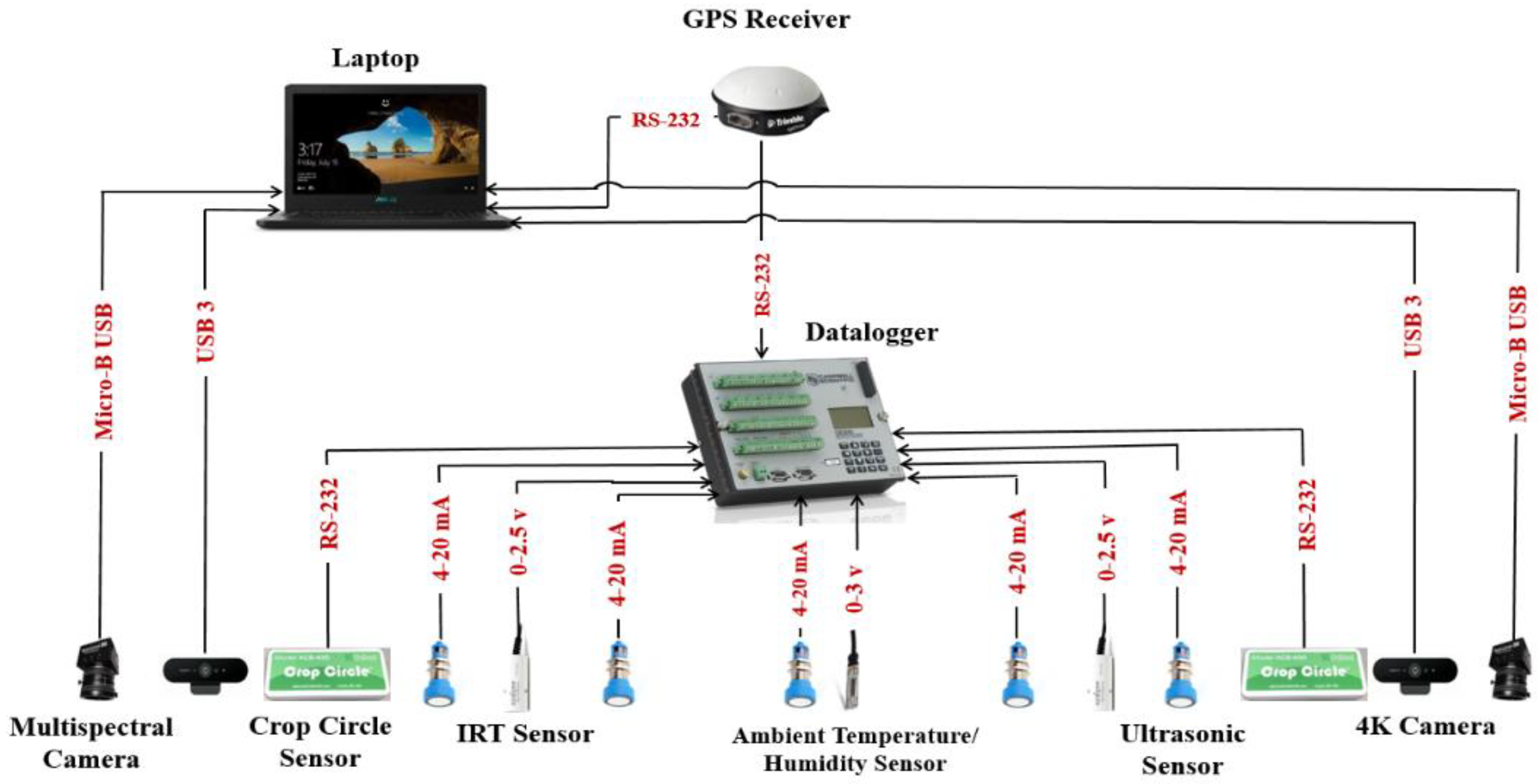
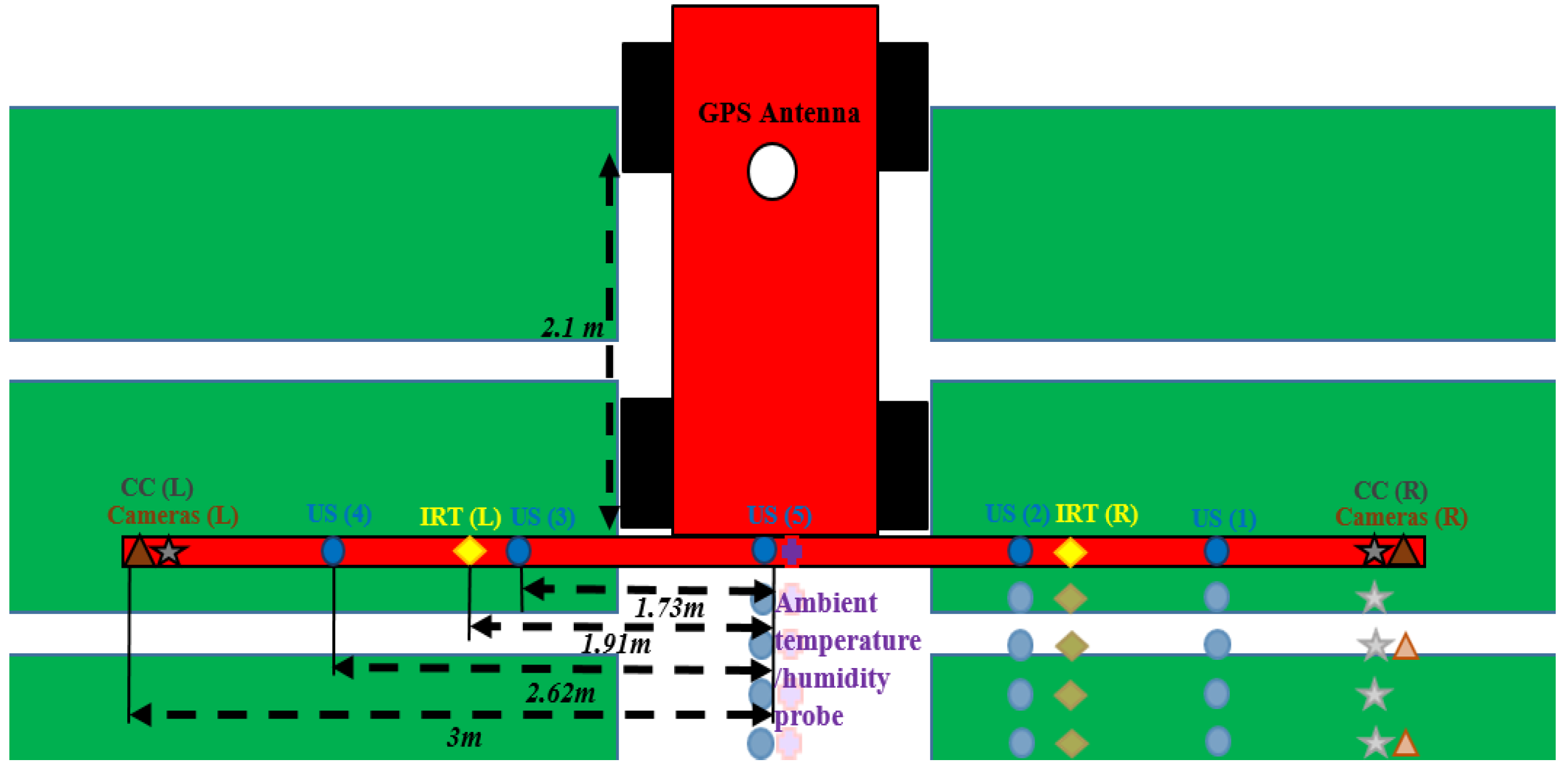
2.1. Electrical Components

The developed HTPP consists of different electrical devices for different purposes. Figure 1 illustrates assembled system for data collections. The main parts are two Crop Circle sensors (Model: ACS-430) for measuring vegetation indices like NDVI (Normalized Difference Vegetation Index), two IRTs (Infra-Red Thermometer) (Model: Apogee SI-131) for measuring canopy’s temperature, a portable weather station (Model: Visala HMP60) for measuring ambient temperature and relative humidity, five ultrasonic sensor (Models: Honeywell 643-F4Y-2D-1D0-180E and Sick UM30-21_113) for measuring the height of canopy, two high quality webcams (Model: Logitech BRIO) for capturing RGB pictures, two multispectral cameras (Model: msCAM CMV4000) for capturing image within specific wavelength ranges, a RTX GPS system for geo-tagging of collected data and images, a Data Logger (Model: Campbell Scientific CR3000) and a laptop computer for executing developed programs to collect and save data/images.

RGB and multispectral cameras are connected to a laptop computer, which works as a central control system and receives GPS signals. All captured images are tagged with their geospatial information and saved into the Laptop computer. Moreover, all sensors’ outputs and GPS string are connected to the Data Logger, which works as other central control system. The captured data are geo-tagged and recorded in the Data Logger. It should be noted that except for the Crop Circle output, which is digital, all other sensors outputs are analog.

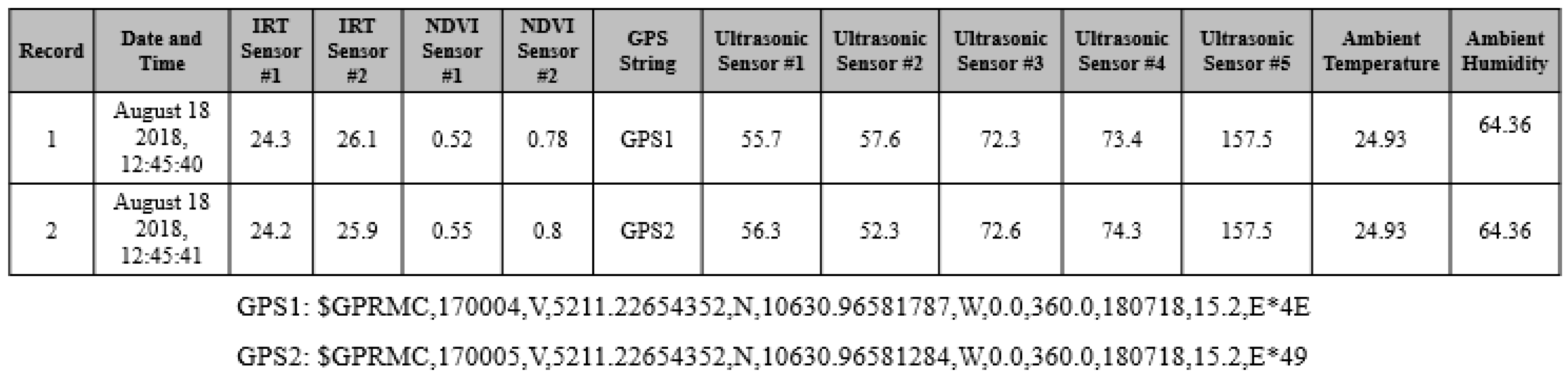
2.1.1. NDVI Measurement by Crop Circle Sensor

The NDVI is a ratio that derives from the reflectance data and is an indicator that quantifies live green vegetation status in different stages of growth. In other words, this indicator demonstrates green vegetation index of an area. NDVI management has several advantages like providing accurate growth trending, frost damage detection, biomass production, canopy coverage, and density detection.

NDVI ratio can be ranged from 0 to +1 or −1 to +1. By selecting 0 to +1 range, computational savings of 15–30% are possible, which is significant for processing of vast amounts of data [12]. Therefore, in this study, we are interested in calculating NDVI in the range of 0 to +1. When NDVI value is close to 0, it means there is no green vegetation in the observed area. On the other hand, if NDVI value is close to +1, highly likely dense green leaves exist in the area. For this range, utilized Crop Circle sensor measures NDVI index from following equation:

$$\mathrm{NDVI}=\frac{NIR-Red}{NIR+Red}$$

(1)

where Red and NIR are two basic spectral reflectance information of red and near-infrared wavelengths, respectively.

2.1.2. Temperature and Humidity Measurement by Infra-Red Thermometer and Weather Station

These sensors are able to measure ambient and crop’s temperature without damaging them in the outdoor applications. Theses sensors do not need any field calibration before start of data collections. The manufacturer usually prepares a product-specific parameter calibration for calculating the temperature. An internal circuit in the sensor works as thermistor, and its resistor changes with temperature. The temperature is calculated as

$$T_T{}^4-T_D{}^4=m.S_D+b$$

(2)

$$m=C_2. T_D{}^2+C_1. T_D+C_0.$$

(3)

$$b=C_2. T_D{}^2+C_1. T_D+C_0$$

(4)

$$T_T={\left(T_D{}^4+m.S_D+b\right)}^{\frac{1}{4}}-273.15$$

(5)

where $C_0$, $C_1,$ and $C_2$ are the custom calibration coefficients that are different for each model of IRTs. $T_T$ is target temperature in Kelvin, $S_D$ is millivolt signal of the detector, and $T_D$ is detector temperature in Kelvin. Furthermore, relative ambient humidity is calculated from

$$RH=\frac{e}{e_s}\times 100$$

(6)

where RH is relative humidity; $e$ is the vapor pressure in kPa, which is an absolute amount of water vapor in the air and is related to the dew point temperature; $e_s$ is the saturation vapor pressure in kPa, which is the maximum value of water vapor that air can hold at a given air temperature.

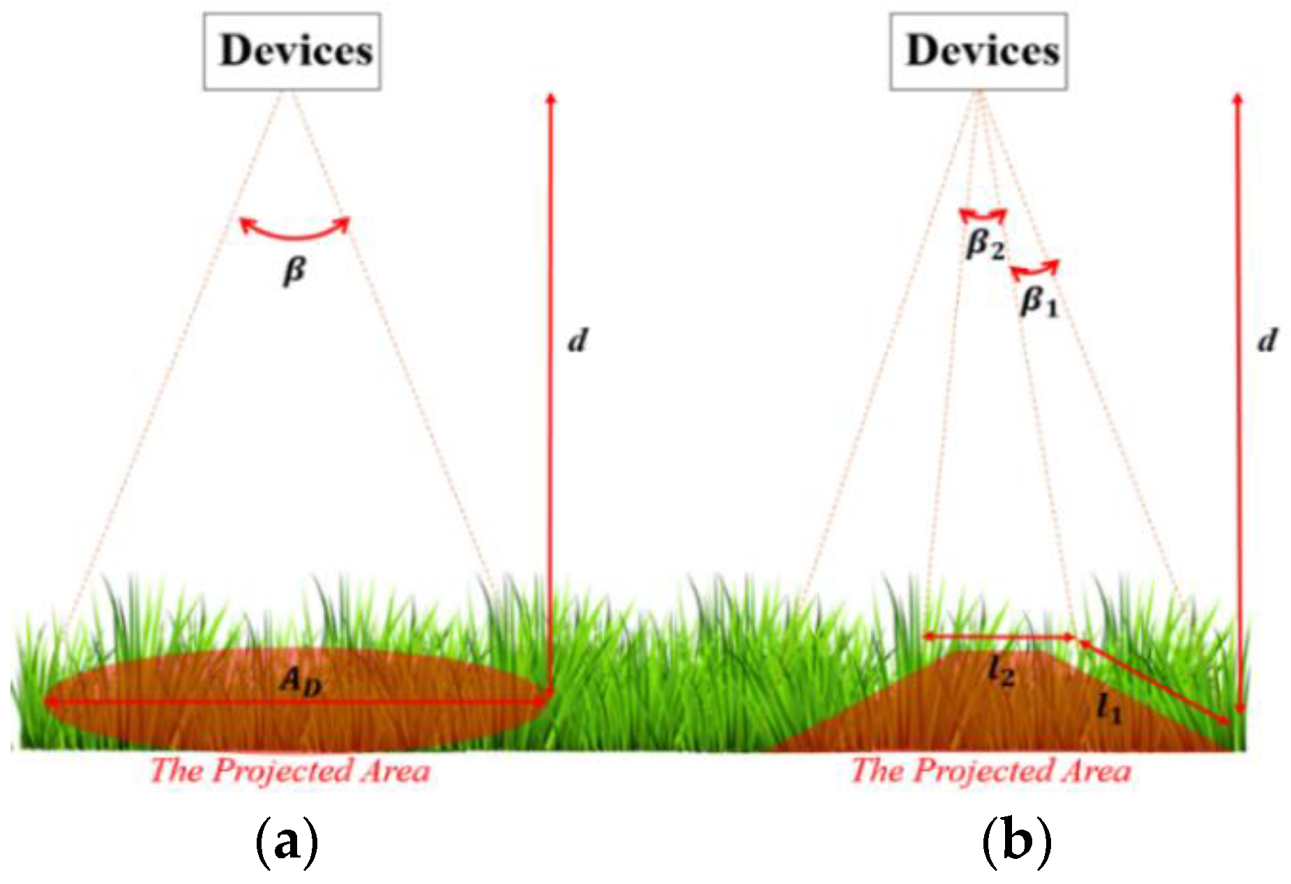
2.1.3. Height Measurement by Ultrasonic Sensor

Ultrasonic sensor measure distances by sending an ultrasound wave and receiving its reflected wave. The traveling time prepares an information about distance between sensor and object, as

$$Y_{US}=\frac{1}{2}\left(S\ast t_{US}\right)$$

(7)

where S is the traveling speed of sound (~343 m/s in dry air 20 °C), $t_{US}$ is traveling time, and $Y_{US}$ is distance between the object and sensor. The output of sensor ($X_{US}$) is a raw data (current), and relationship between the output of sensor and the distance of the object is linear. Therefore, an equation between the sensor’s output and height of objects is modeled by linear regression as

$$Y_{US}=\left(A\ast X_{US}\right)+B$$

(8)

where A and B are coefficients that can be found by measuring at least three different distances and relating them to the corresponding values. Two methods for height measurement were used, the main difference between them being the existence of an extra ultrasonic sensor. The methods are the following:

Method 1—Using four ultrasonic sensors: This approach is valid if distance between the ground and location of the sensor is fixed during the height measurement. By subtracting the distance between the ground and sensor location from the distance between top of object and the location of the sensor, object height is calculated. Before using sensors, they should be calibrated; this sometimes prolongs preparation for field measurements.

Method 2—Using five ultrasonic sensors: In this method, height of crops is measuring without any sensitivity to the variations of mechanical boom’s height, which carries sensors. In this method, distance measurement is used instead of height measurement. By using two sensors, distance value for each sensor is measured. $Y_{US1}$ is distance between the tip of the sensor and ground, and $Y_{US2}$ is distance between the tip of the sensor and object. These values are measured as

$$Y_{US1}=\left(A_1\ast X_{US1}\right)+B_1$$

(9)

$$Y_{US2}=\left(A_2\ast X_{US2}\right)+B_2$$

(10)

where $X_{\mathrm{US}1}$and $X_{\mathrm{US}2}$ are current values (outputs of sensors); A₁, A₂, B₁ and B₂ are coefficients that should be found by measuring the distance values of at least three different objects and relating them to the corresponding values. The height of object (h) is measured as

$$h=Y_{US1}-Y_{US2}=\left(A_1\ast X_{US1}\right)-\left(A_2\ast X_{US2}\right)+B_1-B_2$$

(11)

Therefore, by using this approach, ultrasonic sensors do not need any calibration before start of data collections. This approach was tested for both model of ultrasonic sensors, and by changing height of mechanical boom, height measurement was performed properly and accurately.

All sensors and cameras are attached on the mechanical boom as can be seen in Figure 2. IRT, US, and CC stand for Infra-Red Thermometer, Ultrasonic Sensor and Crop Circle, respectively. The projected area of devices varies by increasing or decreasing height of mechanical boom (Figure 3) and can be calculated as

$$The projected area \left(IRT or US\right)=A_D\times \pi =2\times d\times \tan \left(\frac{\beta }{2}\right)$$

(12)

$$The projected area \left(CC\right)=l_1\times l_2=d^2\times \tan \left(\frac{{\beta }_1}{2}\right)\times \tan \left(\frac{{\beta }_2}{2}\right)$$

(13)

In Equations (13) and (14), d is the distance between sensor and the plant, and $\beta$ is an angular FOV (Field of View), which is different for each device.

Table 1. Summary of major specifications of the utilized measuring devices and their projected areas in two ranges.

Device Type	Response Time (s)	Output Signal	Beam Angle	The Projected Area (m2)
				Sensor to Canopy Range 0.8 (m)	Sensor to Canopy Range 1.3 (m)
Ultrasonic Senor	0.25	Analog (4–20 mA)	$\beta$ = 8°	0.11	0.18
Infra-Red Thermometer	0.60	20 µv per °C	$\beta$ = 28°	0.39	0.64
Crop Circle	0.05	Digital (string)	${\beta }_1$ = 30° ${\beta }_2$ = 14°	0.021 1	0.056

¹ See Equation (13) and Figure 3 for calculation.

represents the summary of major specification of sensors and their projected areas in two sets of ranges.

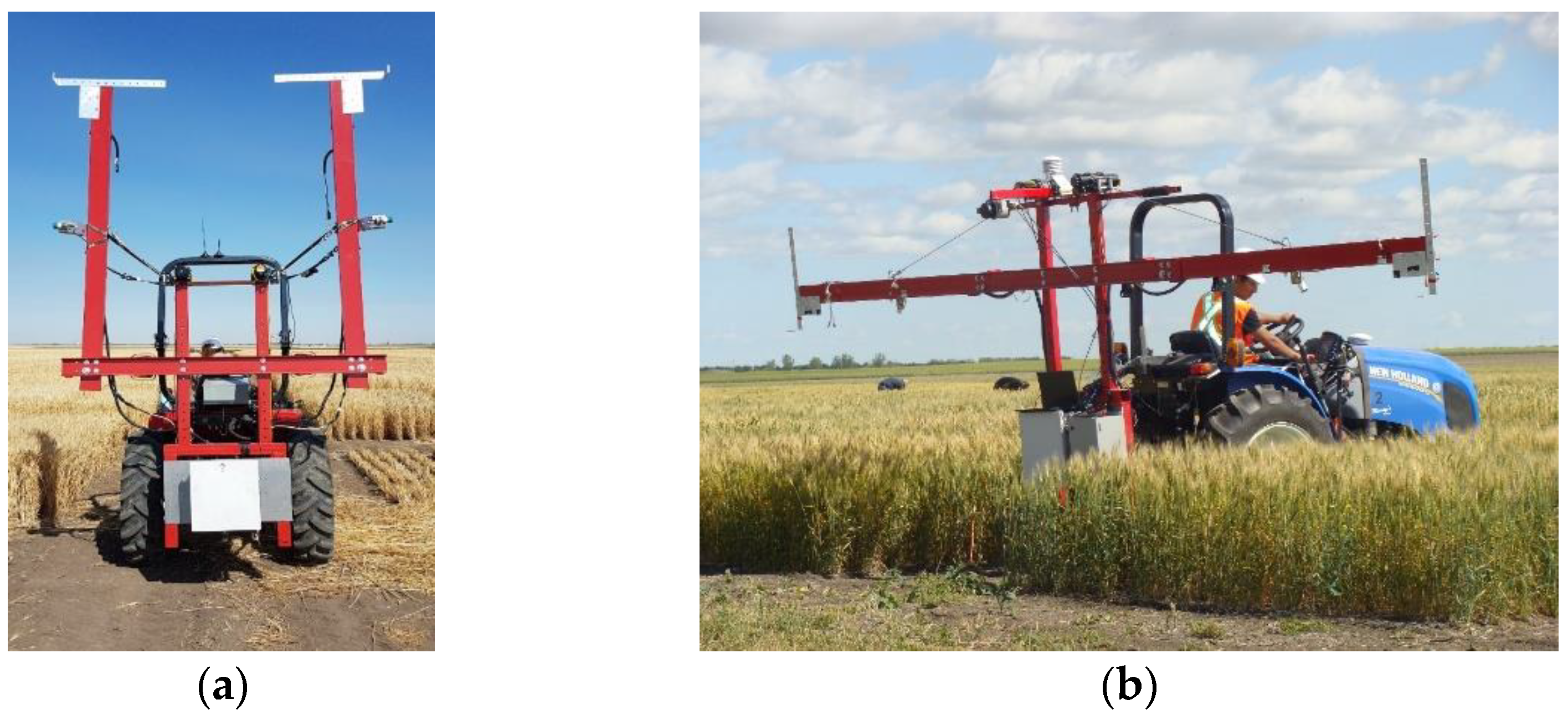
2.2. Mechanical System

The developed ground based HTPP consists of a 6 m (20-feet) long boom, to which sensors and cameras are attached, and a 6-feet wide Tractor, which carries the boom and has highly accurate RTX-GPS as shown in Figure 4. Tractor is semi-autonomous and has auto-steer navigation system, with help from an RTX-GPS system with an accuracy of about 1 inch. Collected data are geo-referenced to the plot level using GPS system. There is a published work, which tested RTX-GPS system, and showed its accuracy is about 1 inch [13]. During the field tests, both left- and right-side sensors and cameras of the boom were able to collect data/pictures, as shown in Figure 2.

The platform uses tractor’s compensating mechanism for auto steering. Different factors, such as speed, sensor locations, and road conditions on the vibration of system, were studied and analyzed. Several vibration tests were done by our team for different speeds of vehicle (1, 1.6, 3.2 mph); it was found that system can collect data reliably with reasonably good accuracy in vehicle constant speed. In addition, it was found that when the tractor speed is 1.6 mph (0.71 m/s), the measurement devices could collect data reliably without any delay or missed GPS data. At higher speed (3.2 mph), although data were collected faster, quality of collected data was compromised. Therefore, vehicle’s speed was set to 1.6 mph (0.71 m/s) during data collections.

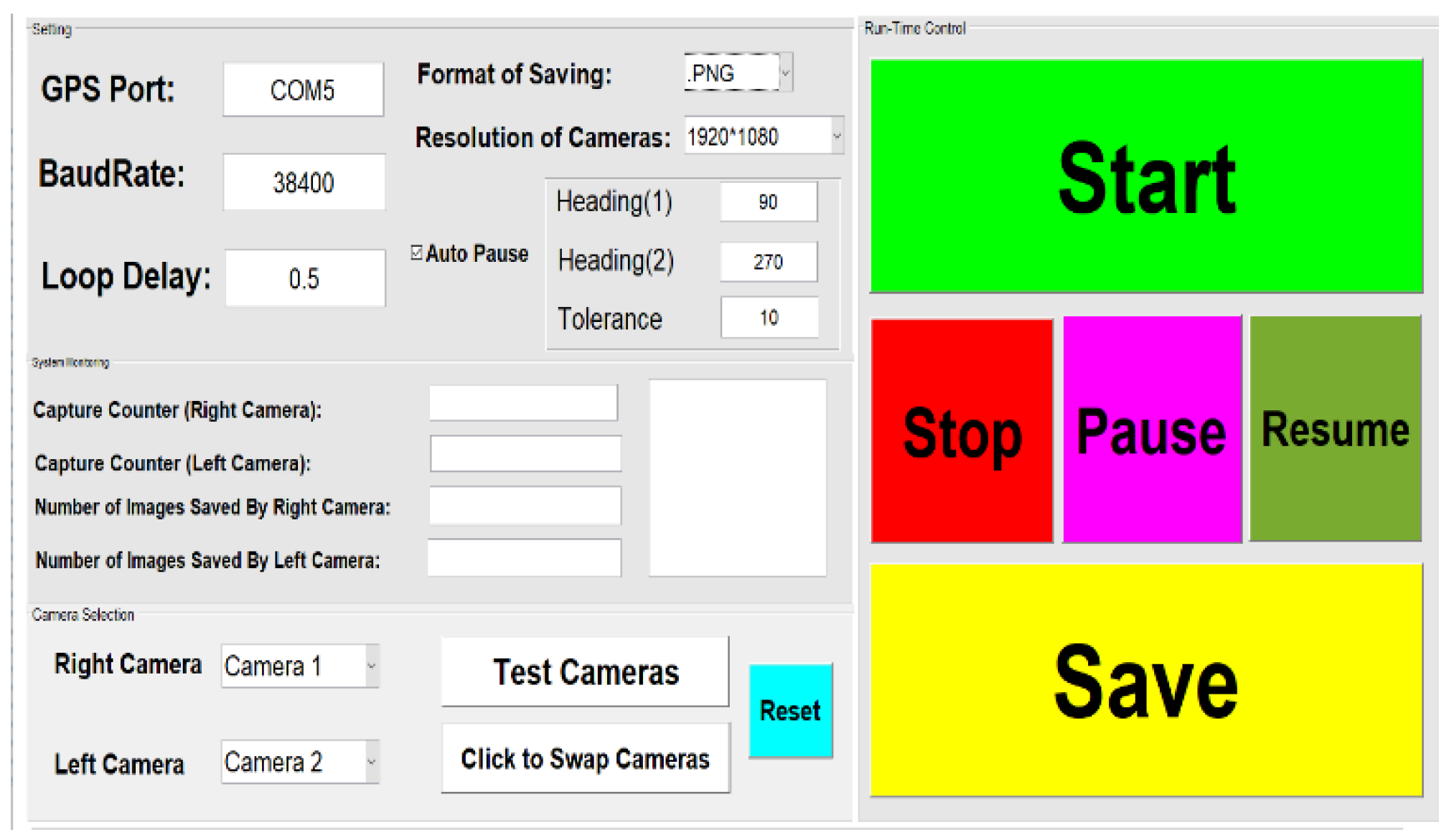
2.3. Software Development

A software package, which was named Pheno-VISDM2 (Visualization, Image acquisition, Sorting and Data acquisition, Mapping), was developed for this research. This package has several modules, which are reflected in the name. In this research, MATLAB was used as the main programming language for developing software for operation of our system. Furthermore, another programming language (CRBasic) was used for data acquisition program. Most of developed programs were executed in the onboard Laptop and Data Logger during data collections. Further, data visualization module was used to monitor and sort collected information.

The baud rate to communicate with the utilized measurement devices is fixed to 38,400 bps (bits per second) to have reliable communication. The data acquisition cycle in the data and image acquisition programs are respectively 250 and 500 ms. In other words, four and two sample points are captured per second during data and image acquisition cycles. The number of collected data for each plot can be determined by selecting proper speed for the vehicle. When the speed of vehicle is set to 1.6 mph (0.71 m/s), proper amount of data is collected using each device (GPS receiver, sensors, and cameras). For this speed, the required time for vehicle to pass through a single plot (1.2 m wide) is 1.71 sec. If 0.25 s is what takes for 1 sample data to be recorded, then for each plot, with vehicle travelling time of 1.71 s, platform captures 6.8 records of data. These numbers can vary based on availability of GPS signal.

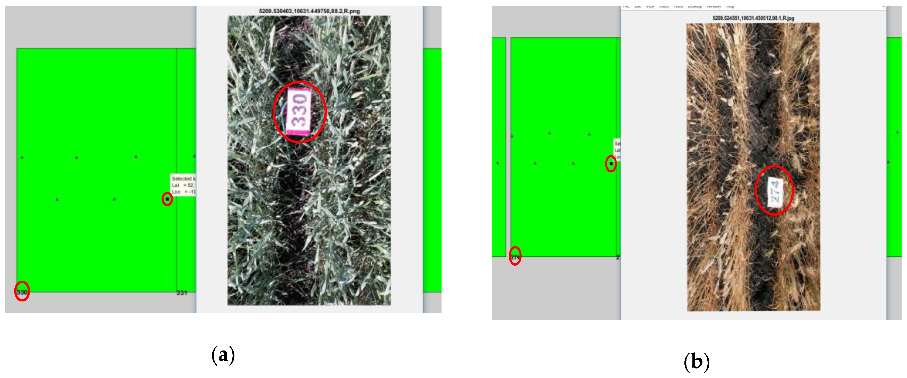
2.3.1. Image Acquisition Module

Different image acquisition programs were developed to capture RGB and multispectral images. In this paper, RGB image acquisition program is discussed. To develop this program, image acquisition toolbox of MATLAB was employed. The main command that was used is snapshot. This command acquires single image frame from the connected webcams. By calling snapshot in a loop, a new frame will be captured in each iteration. Two versions of programs were developed in MATLAB GUI (Graphical User Interface) to communicate with the webcams.

First version of image acquisition was developed previously by Robotics group of Mechanical Engineering Department of University of Saskatchewan [14]. The second version is more automated and user friendly and also has more features. As can be seen in Figure 5, user can select format of saving (.jpg and png) and resolution of webcams (640 × 360, 960 × 540, 1280 × 720, and 1920 × 1080).

Table 2. Time spent in saving RGB images with different resolutions and formats. Moreover, number and size of captured images are compared.

No.	Resolution	Format	Size of Each Picture (Average)	Number of Captured Images	Size of Captured Images	Required Time for Saving Images on the Hard Drive
Test 1	1920 × 1080	.png	4 MB	1658	6.55 GB	16:00
Test 2	1920 × 1080	.jpg	600 KB	1656	885 MB	1:30
Test 3	1280 × 720	.png	2.2 MB	1640	3.13 GB	6:00

shows required time for saving images with different resolutions and formats. Moreover, in this version, user can pause the capture cycle of image acquisition and resume it, manually. However, the main advantage of new version image acquisition program is the existence of auto-pause feature. Because the output of GPS receiver is connected to the laptop, GPS string is used for geo-tagging, and the heading angle of vehicle is extracted from this string. By using auto-pause option, program is going to be paused automatically in the places where vehicle is turning. User can determine two valid headings for the vehicle and tolerance values for them. For example, in Figure 6, by determining 90 degree for Heading 1, 270 degree for Heading 2, and 10 degree for Tolerance, image acquisition program will work for the headings that are between 80 and 100 degrees and 260 and 280 degrees. Thus, image acquisition program should be paused automatically, when vehicle is in position 3 or 4.

This program was tested and used in laboratory conditions and during field experiments. It was found that the program is working reliably and accurately.

Table 3. Comparison between the operation of developed image acquisition program for RGB images with and without auto-pause option for the entire studied wheat field.

No.	Mode of Image Acquisition Program	Format	Number of Captured Images
Test 1	With auto-pause feature	.png	1900
Test 2	Without auto-pause feature	.png	2400

compares number of captured images with and without auto-pause option for the studied wheat field, which comprised from 9 rows (total amounts of plots were 270). From this table, it can be said that by using the auto-pause feature, the image acquisition system captures just proper and valid images, and as a result, less time is needed for saving action, which is more than 20% improvement in saving time.

2.3.2. Data Acquisition Module

This program controls in the Data Logger to collect sensor’s data (ultrasonic, infrared thermometer, Crop Circle, ambient temperature, and humidity sensors) and creates phenotypic database as shown in Figure 7. Each row of this table (record) consists of data collection’s time information, GPS string, and sensors’ values. The number of records depends on the size of monitored field and the duration of data collection. IRT #1 (right) and IRT #2 (left) sensor columns encompass collected temperature of crops via infrared thermometers. NDVI sensor #1 (right) and 2 (left) columns represent the captured NDVI value by each sensor. Moreover, ultrasonic sensors #1–2 (right) and #3–4 columns show the height of canopies that are recorded by the related sensors. Ultrasonic sensor #5 (center) column represents height of boom during the data collection. GPS string column represents NMEA (National Marine Electronics Association) GPS string of each record. Collected data is related to the plot level in the future retrieval, by use of recorded geospatial information.

To develop a data acquisition program, a software called LoggerNet (Version 4) was utilized. This software is provided by the manufacture of Data Logger (Campbell Scientific, Logan, UT, USA) and is used for writing and compiling codes (the programming language is CRBasic).

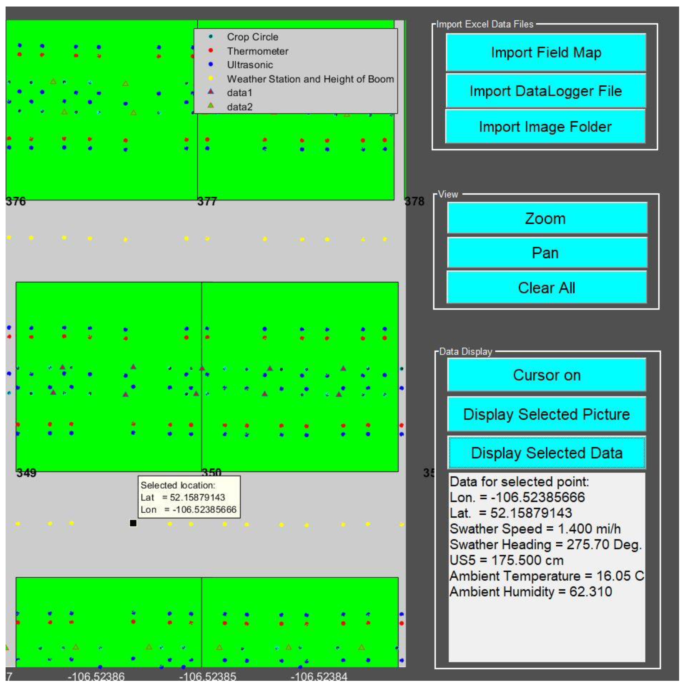
2.3.3. Visualization Module

To analyze and monitor collected data and images, a data visualization program was developed. This program has several buttons, as shown in the right side of Figure 8 with blue colors. The program is used to import and monitor field map. The target-monitoring field was mapped by RTX-GPS in a previous stage. An Excel file, which has geospatial information of each plot of the monitored wheat field, should be used for importing the map of field in the visualization module [11,14]. All collected data and images, which are geo-tagged during the data collection phase, are loaded through this module for post-processing. Moreover, using this program, geo-referencing of the collected data/images was verified, which will be discussed in the results section.

All longitude and latitude values used for tagging (for data and image) are in degrees-minutes format ($La{t}_{DM}$/$Lo{n}_{DM}$). They need to be converted to decimal degrees ($La{t}_{DD}$/$Lo{n}_{DD}$) by using the following equations (using floating point numbers) [15,16]:

$$La{t}_{DD}=\left(\frac{La{t}_{DM}-5200}{60}\right)+52$$

(14)

$$Lo{n}_{DD}=\left(\left(\frac{Lo{n}_{DM}-10600}{60}\right)+106\right)\times \left(-1\right)$$

(15)

As can be seen in Figure 9, latitude and longitude of a point (e.g., P2) can be related to another point (e.g., P1) on the Earth surface using the following relations [14]:

$$la{t}_{D{D}_2}={\sin }^{-1}[\cos \left(\theta \right)\cos \left(la{t}_{D{D}_1}\right)\sin \left(\delta \right)+\sin \left(la{t}_{D{D}_1}\right)\cos \left(\delta \right)]$$

(16)

$$lo{n}_{D{D}_2}=lo{n}_{D{D}_1}+{\tan }^{-1}(\frac{\cos \left(la{t}_{D{D}_1}\right)\sin \left(\theta \right)\sin \left(\delta \right)}{\cos \left(\delta \right)-\sin \left(la{t}_{D{D}_1}\right)\sin \left(la{t}_{D{D}_2}\right)})$$

(17)

$$\delta =\frac{k}{R}$$

(18)

The $la{t}_{D{D}_1}$ and $lo{n}_{D{D}_1}$ are latitude and longitude at P1; $la{t}_{D{D}_2}$ and $lo{n}_{D{D}_2}$ are latitude and longitude at P2; $\theta$ is vehicle’s heading angle with respect to the Earth magnetic north pole; k is distance between P1 and P2, and R is the Earth’s radius in meter (assuming earth is a complete sphere, radius = 6371 km). This approach (Equations (16)–(18)) gives exact locations of each sensor, which is then used to load data/images into the visualization module. After loading data and images, green and red triangles and blue, black, and red dots appear on the screen. They represent, respectively, locations of left and right cameras, ultrasonic, Crop Circle, infrared thermometer sensors. By selecting any of these icons, the measured data and captured images can be visualized. Furthermore, yellow dots are used to show height of the boom, ambient temperature, and humidity (Figure 8).

3. Results

In this section, operational quality and usefulness/efficiency of this ground-based mobile HTPP is discussed.

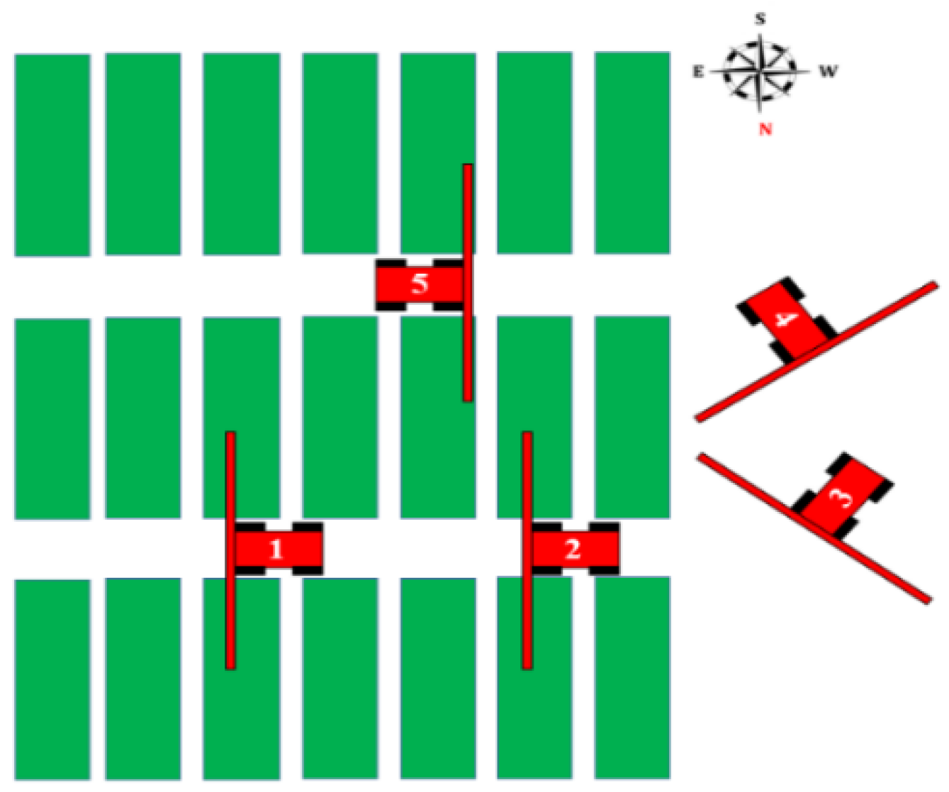
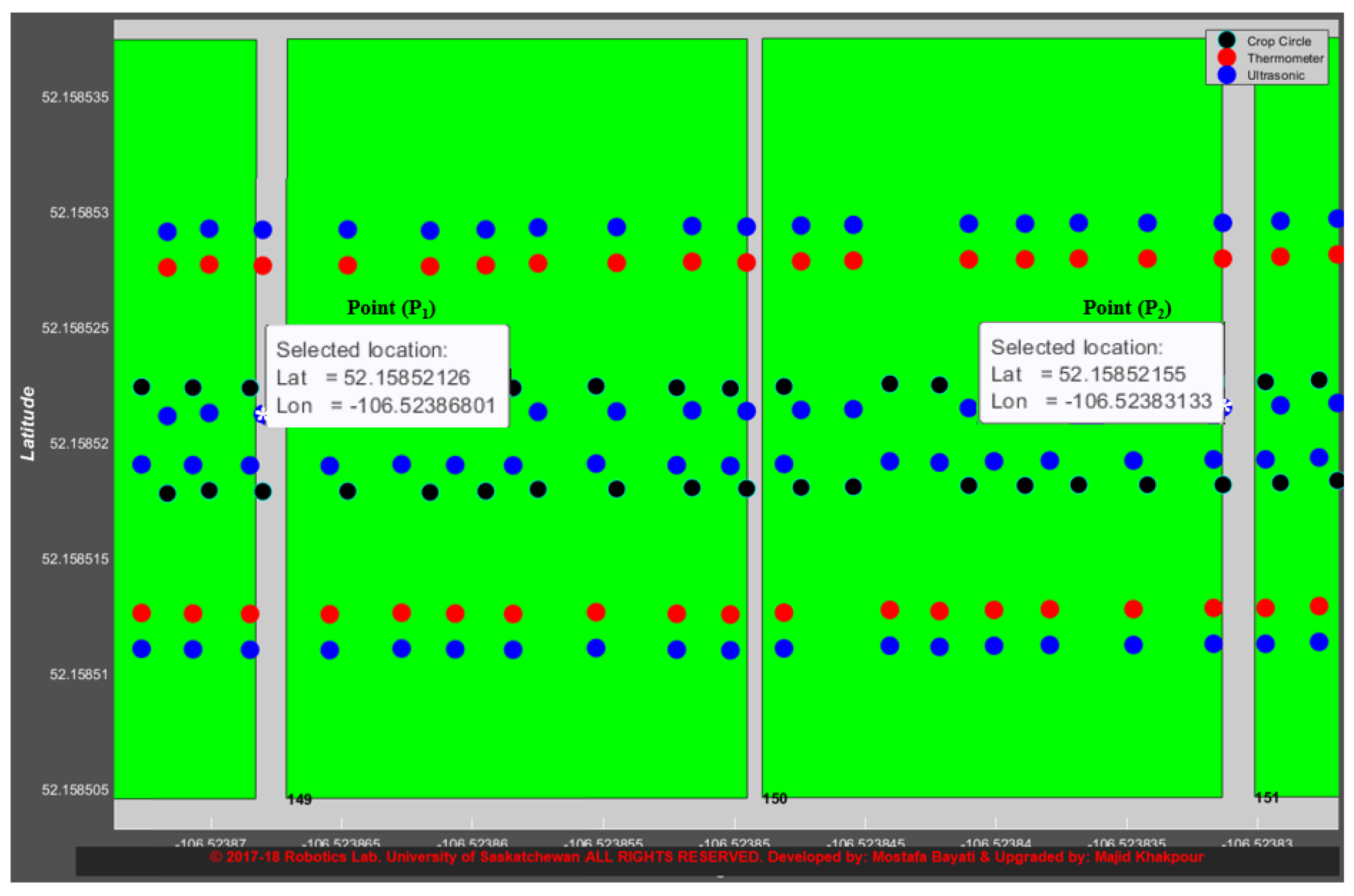
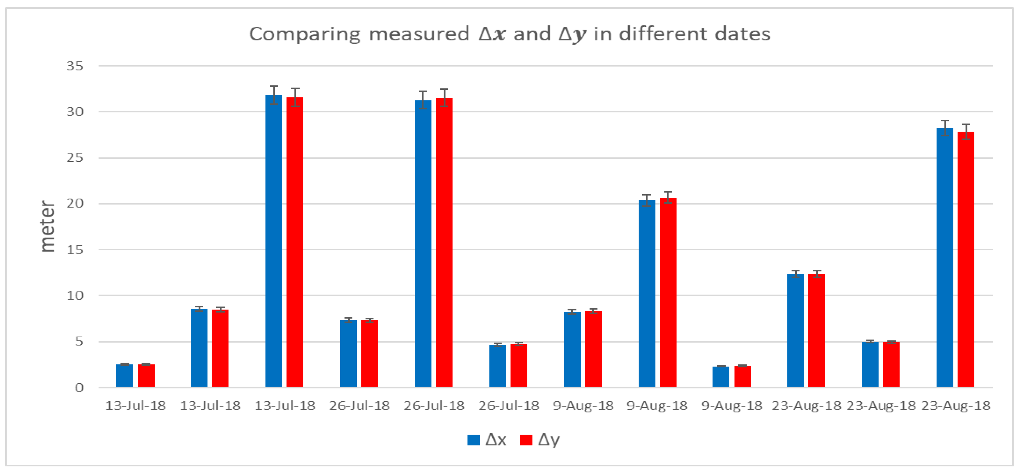
3.1. Verifying the Validity of Geo-Referenced Data

To verify the accuracy of developed HTPP and related programs, 45 physical signs were placed next to different plots, randomly. Each sign had a tag that shows the corresponding plot number. Figure 10 shows the tags set to two plots, while the pictures are loaded into visualization module of Pheno-VISDM2.

3.2. Analyzing Delay in the Process of Geo-Referencing

In this section, delay issue during the process of geo-referencing is discussed. Since the GPS system and devices are synchronized, and they work with the same frequency, the delay issue is almost eliminated. GPS receiver generates NMEA RMC (Recommended Minimum Sentence C) data string, continuously.

As discussed before, the speed of Tractor was set to 1.6 mph (0.71 m/s) in auto-steering mode; the travel speed was constant. Moreover, the time information of each record can be extracted from phenotypic database (Figure 7). Therefore, the distance between points P₁ and P₂ in Figure 11 can be calculated, as Equation (19).

$$\Delta x=v\times \Delta t$$

(19)

where $\Delta t$ is the time differences between record for point P₁ and P₂. For this example (Figure 11), $\Delta t$ is 3.5 s. From Equation (19), $\Delta x$ is founded to be 2.502 m. Additionally, the geospatial information of points P₁ and P₂ are

$$\mathrm{Point} {\mathrm{P}}_1: (la{t}_{D{D}_1}, lo{n}_{D{D}_1})=52.15852126,-106.52386801$$

$$\mathrm{Point} {\mathrm{P}}_2: (la{t}_{D{D}_2}, lo{n}_{D{D}_2})=52.15852155,-106.52383133$$

The distance of two points (Figure 11) can be calculated by use of their geospatial information, as [17]

$$\Delta La{t}_{DD}=la{t}_{D{D}_2}-la{t}_{D{D}_1}$$

(20)

$$\Delta Lo{n}_{DD}=lo{n}_{D{D}_2}-lo{n}_{D{D}_1}$$

(21)

$$\Delta y =2\times \mathrm{R}\times \arcsin \left(\sqrt{{\sin }^2\left(\frac{\Delta La{t}_{DD}}{2}\right)+\cos \left(la{t}_{D{D}_1}\right).\cos \left(la{t}_{D{D}_2}\right).{\sin }^2\left(\frac{\Delta Lo{n}_{DD}}{2}\right) }\right)$$

(22)

where R is Earth’s radius in meters. Therefore, $\Delta y$ is 2.504 m.

Table 4. Examples for analyzing delay in the process of geo-referencing by comparing distances values between two points (P₁ and P₂); ($\Delta x$ −$\Delta y)\%=\frac{\left|\Delta x-\Delta y\right|}{\left(\Delta x+\Delta y\right)/2}$.

Date	$\mathit{l}\mathit{a}{\mathit{t}}_{\mathit{D}{\mathit{D}}_1}$ $\mathit{l}\mathit{o}{\mathit{n}}_{\mathit{D}{\mathit{D}}_1}$	$\mathit{l}\mathit{a}{\mathit{t}}_{\mathit{D}{\mathit{D}}_2}$ $\mathit{l}\mathit{o}{\mathit{n}}_{\mathit{D}{\mathit{D}}_2}$	$\mathbf{\Delta }\mathit{t}\mathbf{\left(}\mathbf{s}\mathbf{\right)}$	$\mathbf{\Delta }\mathit{x}\mathbf{\left(}\mathbf{m}\mathbf{\right)}$	$\mathbf{\Delta }\mathit{y}\mathbf{\left(}\mathbf{m}\mathbf{\right)}$	$\mathbf{\Delta }\mathit{x}$ − $\mathbf{\Delta }\mathit{y}\mathbf{\left(}\mathbf{m}\mathbf{\right)}$	$\mathbf{(}\mathbf{\Delta }\mathit{x}$ − $\mathbf{\Delta }\mathit{y}\mathbf{)}$$\%$
13 July 2018	52.15852155 −106.52383133	52.15852126 −106.52386801	3.50	2.50	2.50	0.00	0.0%
13 July 2018	52.15862831 −106.52383374	52.15862686 −106.52395788	12.00	8.58	8.47	0.11	1.3%
13 July 2018	52.15882397 −106.52377929	52.15882307 −106.52424218	44.50	31.82	31.58	0.24	0.76%
26 July 2018	52.15887304 −106.5240459	52.15887342 −106.52415305	10.25	7.33	7.31	0.02	0.27%
26 July 2018	52.15862818 −106.52378024	52.15862758 −106.52424228	43.75	31.28	31.52	−0.24	0.76%
26 July 2018	52.15852801 −106.52375944	52.15852804 −106.52382901	6.50	4.65	4.75	−0.10	2.1%
9 August 2018	52.15887256 −106.52378121	52.15887294 −106.52390315	11.50	8.22	8.32	−0.10	1.2%
9 August 2018	52.15872534 −106.52377851	52.15872504 −106.52408141	28.50	20.38	20.66	−0.28	1.4%
9 August 2018	52.15847832 −106.52379675	52.15847827 −106.52383171	3.25	2.32	2.38	−0.06	2.6%
23 August 2018	52.15857626 −106.52379588	52.15857759 −106.52397491	17.25	12.33	12.34	−0.01	0.08%
23 August 2018	52.15867586 −106.52393973	52.158677611 −106.52386733	7.00	5.01	4.94	0.06	1.2%
23 August 2018	52.15887199 −106.5238358	52.15887221 −106.52424361	39.50	28.24	27.82	0.42	1.5%

represents more examples on different days, and Figure 12 compares the values of differences ($\Delta x$ and $\Delta y$) of GPS locations of the two points P1 and P2 for these records. Error bars on the diagram represent data variability, and they provide information about the error or uncertainty in the reported measurements. Maximum amount of percentage value ($(\Delta x$−$\Delta y)$%), which is 2.6% of measurements, is considered for adding error bar for each record in the Figure 12.

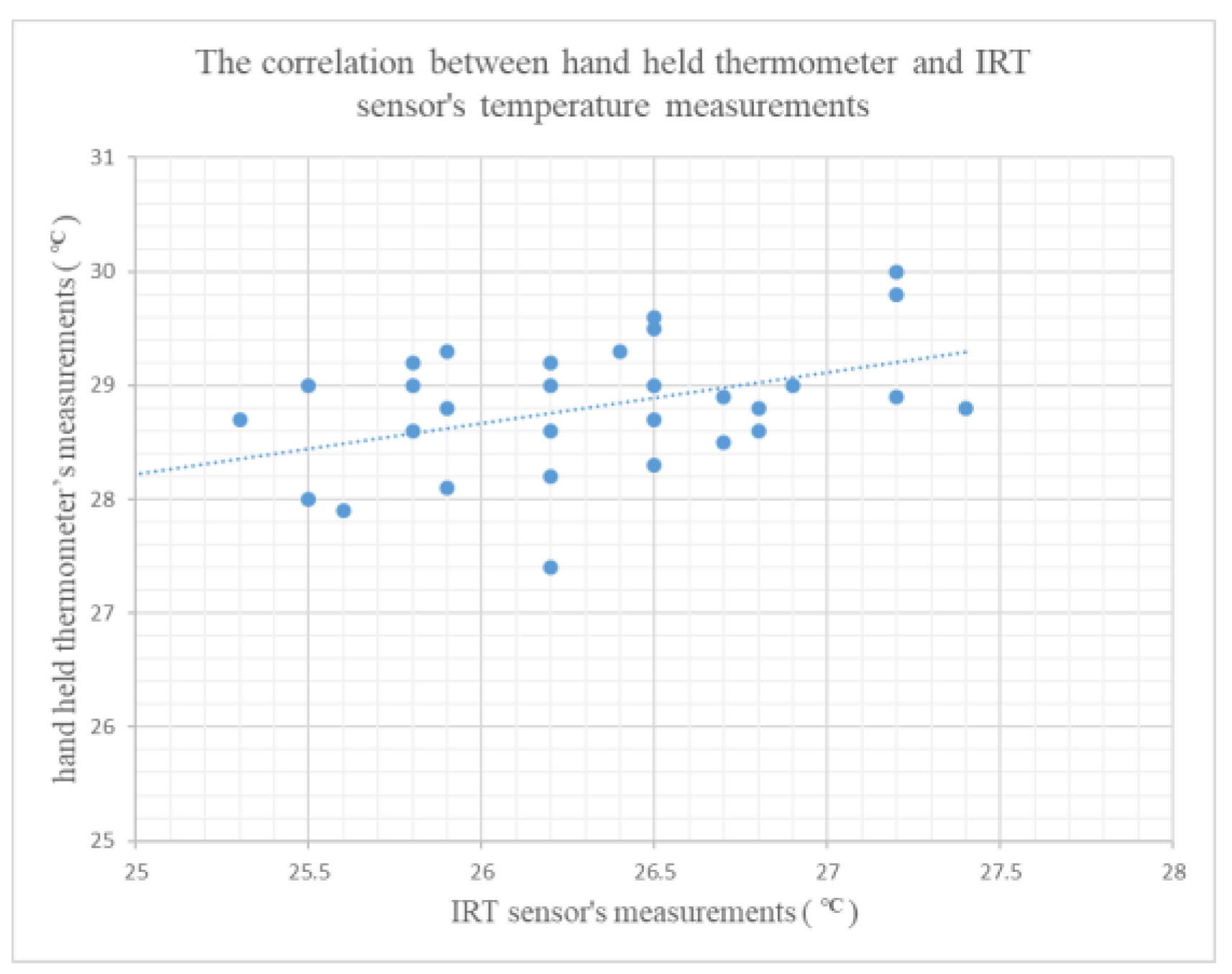
3.3. Accuracy of Crops Temperature Measurement

To verify the validity of HTPP in measuring crop’s temperature, their temperature was measured manually and compared with IRT sensor values. Handheld thermometer sensor (model: IRTC40) was used for manual measurements. Several plots with different genotypes were selected randomly, and their temperature was measured from 4 points, manually.

The angle of measuring device was the same as the IRT sensor during the measurement, and the distance between the handheld thermometer and crops was also almost the same, around 30 cm away. With this distance, both devices have similar fields of view.

Table 5. Comparison between handheld and infrared thermometers’ temperature measurements of different plots on 9 August 2018; “Temp” stands for temperature.

R	Plot Number	Manual Temperature Measurement (°C)				Average of Manual Temp (°C)	Average of IRT Temp (°C)	Diff	%Diff
		Temp 1	Temp 2	Temp 3	Temp 4
1	131	27.5	26	27.4	25.3	26.5	28.3	−1.7	−6%
2	134	27.4	27.2	27.7	27.4	27.4	28.8	−1.3	−5%
3	138	27.7	27.7	27.0	26.7	27.2	28.9	−1.6	−6%
4	147	27.2	25.5	26.8	25.6	26.2	29.0	−2.7	−10%
5	150	28.2	25.8	27.2	26.5	26.9	29.0	−2.0	−7%
6	156	26.8	27.2	26.5	25.8	26.5	29.0	−2.4	−9%
7	165	25.8	26	25.1	25.3	25.5	28.0	−2.4	−9%
8	173	26.0	25.8	25.3	25.3	25.6	27.9	−2.3	−9%
9	176	27.0	26.8	26.7	27.0	26.8	28.8	−1.9	−7%
10	179	27.0	26.8	27.7	27.4	27.2	30.0	−2.7	−9%
11	202	26.0	27.0	26.2	26.8	26.5	29.5	−3.0	−11%
12	212	26.2	26.3	26.5	26.0	26.2	27.4	−1.1	−4%
13	215	26.3	26.0	26.5	26.0	26.2	28.6	−2.4	−9%
14	220	25.8	26.0	26.2	25.8	25.9	28.8	−2.8	−10%
15	224	26.0	26.3	26.8	26.0	26.2	29.2	−2.9	−11%
16	229	25.5	25.6	25.3	27.0	25.8	28.6	−2.7	−10%
17	232	24.7	25.1	24.2	24.8	24.7	27.5	−2.8	−11%
18	237	24.1	24.4	23.5	23.3	23.8	27.6	−3.7	−15%
19	246	26.5	25.0	26.6	25.3	25.8	29.2	−3.3	−12%
20	251	25	23.5	24.4	24.8	24.4	28.3	−3.8	−15%
21	259	27.7	26.3	27.5	26.0	26.8	28.6	−1.8	−6%
22	268	27.5	26.2	27.0	27.0	26.7	28.9	−2.1	−7%
23	271	26.5	26.2	27.0	26.5	26.5	28.7	−2.1	−7%
24	274	27.0	27.4	27.2	27.5	27.2	29.8	−2.5	−9%
25	277	26.5	26.3	26.2	26.0	26.2	28.2	−1.9	−8%
26	304	25.7	26.5	23.5	23.0	24.6	28.2	−3.5	−13%
27	307	25.3	25.0	23.9	24.1	24.5	27.8	−3.2	−12%
28	313	26.5	25.8	26.2	25.1	25.9	29.3	−3.4	−12%
29	320	25.8	25.0	25.5	27.0	25.8	29.0	−3.1	−12%
30	325	25.5	25.0	25.5	25.3	25.3	28.7	−3.3	−12%
31	330	26.8	26.7	26.8	26.5	26.7	28.5	−1.8	−7%
32	333	26.0	26.2	25.8	25.8	25.9	28.1	−2.1	−8%
33	338	26.7	26.5	26.5	26.3	26.5	29.6	−3.1	−11%
34	345	26.5	26.0	26.7	26.8	26.4	29.3	−2.8	−11%
35	352	25.6	25.5	25.1	25.8	25.5	29.0	−3.5	−13%
36	358	26.0	25.5	25.3	25.1	25.4	28.6	−3.1	−12%
37	365	25.8	25.1	25.3	25.6	25.4	28.8	−3.3	−12%
38	373	26.2	26.8	25.8	27.5	26.5	29.3	−2.7	−10%
39	377	27.0	25.5	25.6	25.6	25.9	28.9	−2.9	−11%
40	380	26.1	24.8	25.0	24.4	25.0	28.5	−3.4	−13%

shows an example for comparison between manual and IRT temperature measurements for wheat field on 9 August 2018 (Temp stand for temperature). Diff and %Diff are calculated from

$$Diff=Average of Manual Temp-Average of IRT Temp$$

(23)

$$\% Diff=\frac{Diff}{\left(Average of Manual Temp+Average of IRT Temp\right)/2}$$

(24)

Correlation is a statistical relationship between two quantitative variables. This coefficient is a number between 0 and +1 or −1 and 0. Figure 13 shows the spectrum of the correlation coefficient (−1 to +1) [18]. In this study, positive correlation approach is used for comparing manual measurements with sensor’s data. The correlation coefficient of +1 indicates perfect or strong relation, and 0 means no relationship between two variables. The correlation value (r) can be calculated from Pearson’s correlation coefficient formula as can be seen in Equation (25) [19].

$$r=\frac{n\left({{\displaystyle \sum }}_{i=1}^n{p}_i{q}_i\right)-({{\displaystyle \sum }}_{i=1}^n{p}_i)({{\displaystyle \sum }}_{i=1}^n{q}_i)}{\sqrt{n{{\displaystyle \sum }}_{i=1}^n{p}_i{}^2-{({{\displaystyle \sum }}_{i=1}^n{p}_i)}^2}\sqrt{n{{\displaystyle \sum }}_{i=1}^n{q}_i{}^2-{({{\displaystyle \sum }}_{i=1}^n{q}_i)}^2}}$$

(25)

where $p_i$ and $q_i$ are values of variables indexed with i, and n is number of values for each variable. Figure 14 shows scatter diagram for temperature measurements comparison for different wheat plots on 31 July 2018.

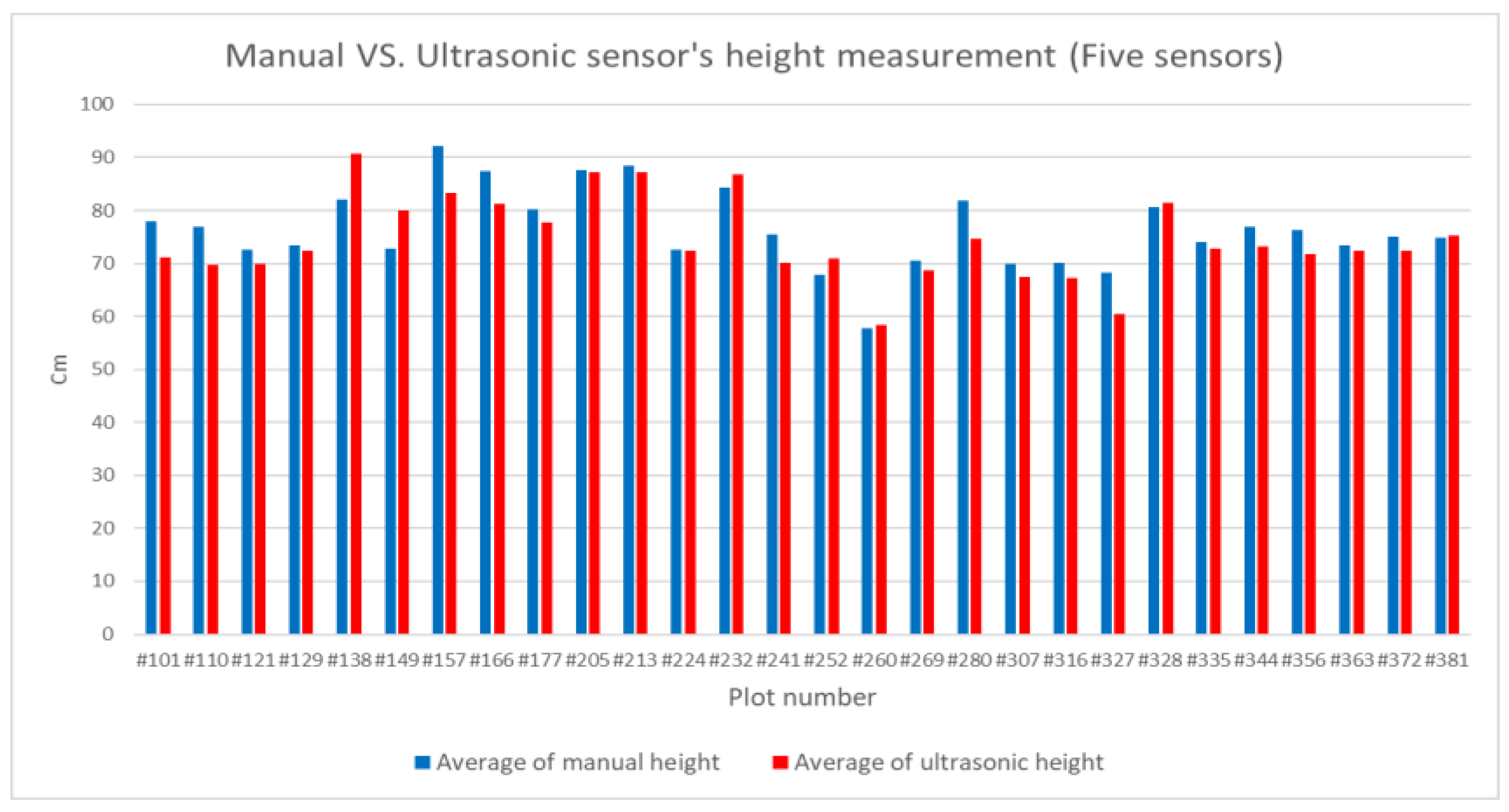
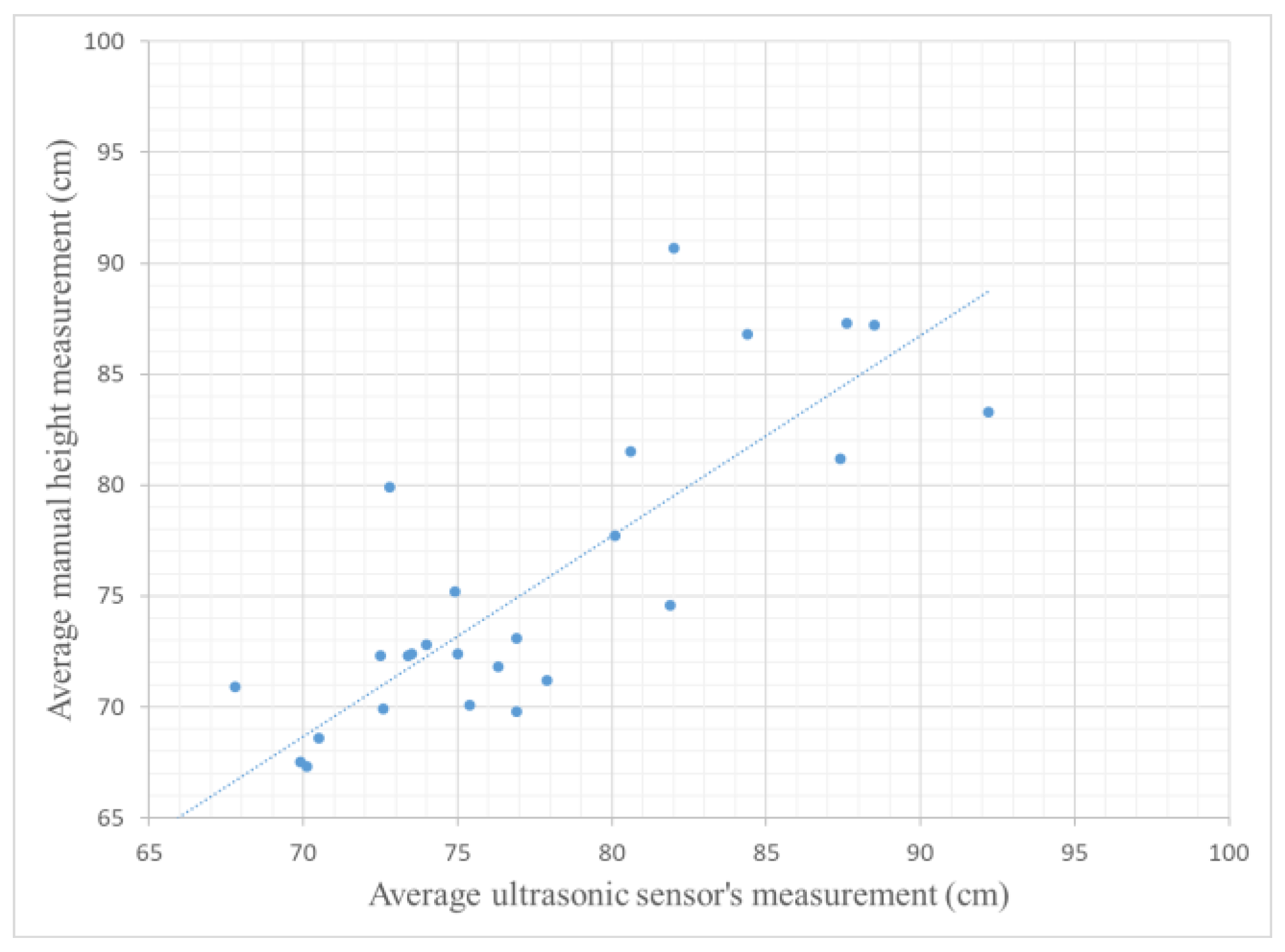
3.4. Accuracy of Crops Height Measurement

In this section, the validity of ultrasonic sensor is discussed. The results of manual and ultrasonic sensor height measurements are provided. For manual height measurement, crops height was measured in three different locations inside each plot, and the averages of these three measurements were calculated and used. Ultrasound height measurement was discussed in detail in Section 2.1. These sensors collected between 15 and 20 data points for each plot with two trips per plot (each trip covered half of each plot). Since breeding field train is rough, sometimes it caused boom tilt. Consequently, there are differences in 15 to 20 measured points.

Collected data using two different measurement methods, as explained in Section 2.1, were compared with manual measurements for 28 random plots as can be seen in Figure 15. Figure 16 shows the scatter diagram for height measurement comparison of different wheat plots (both ultrasonic methods).

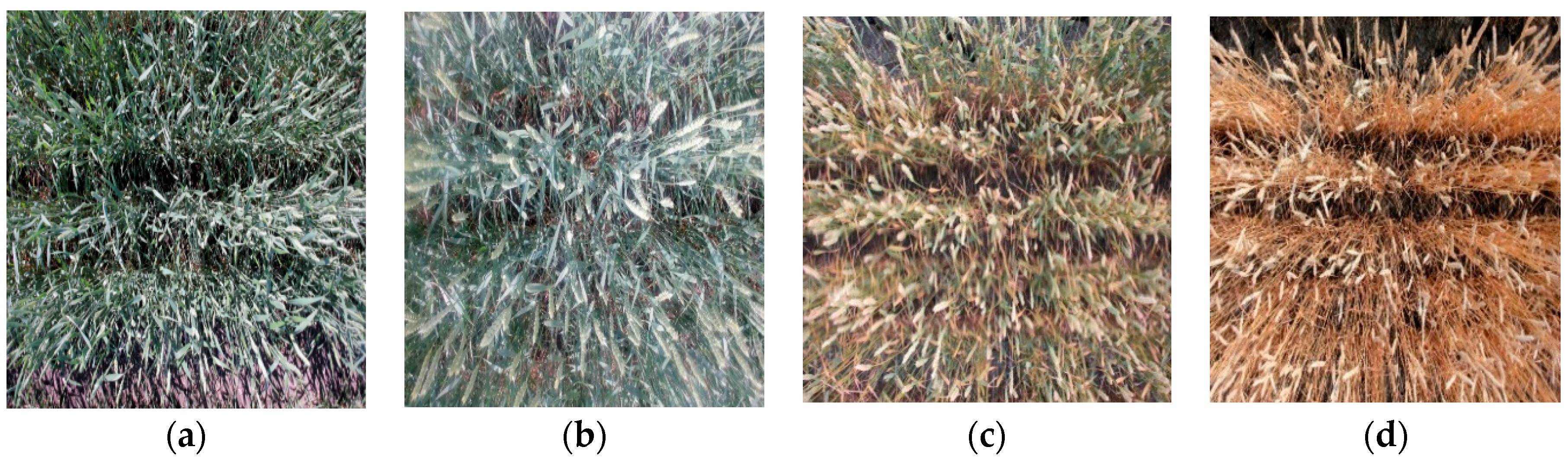
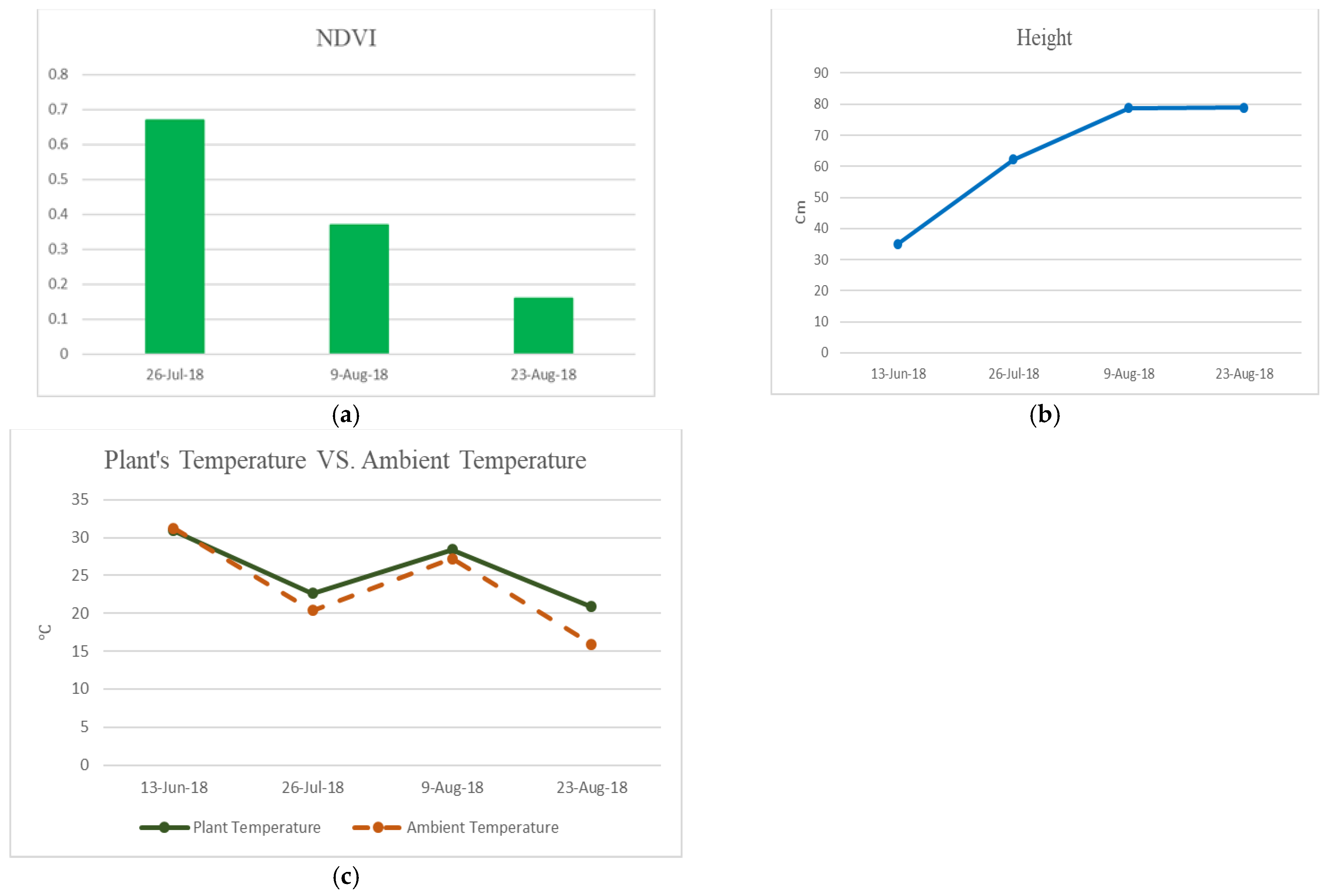
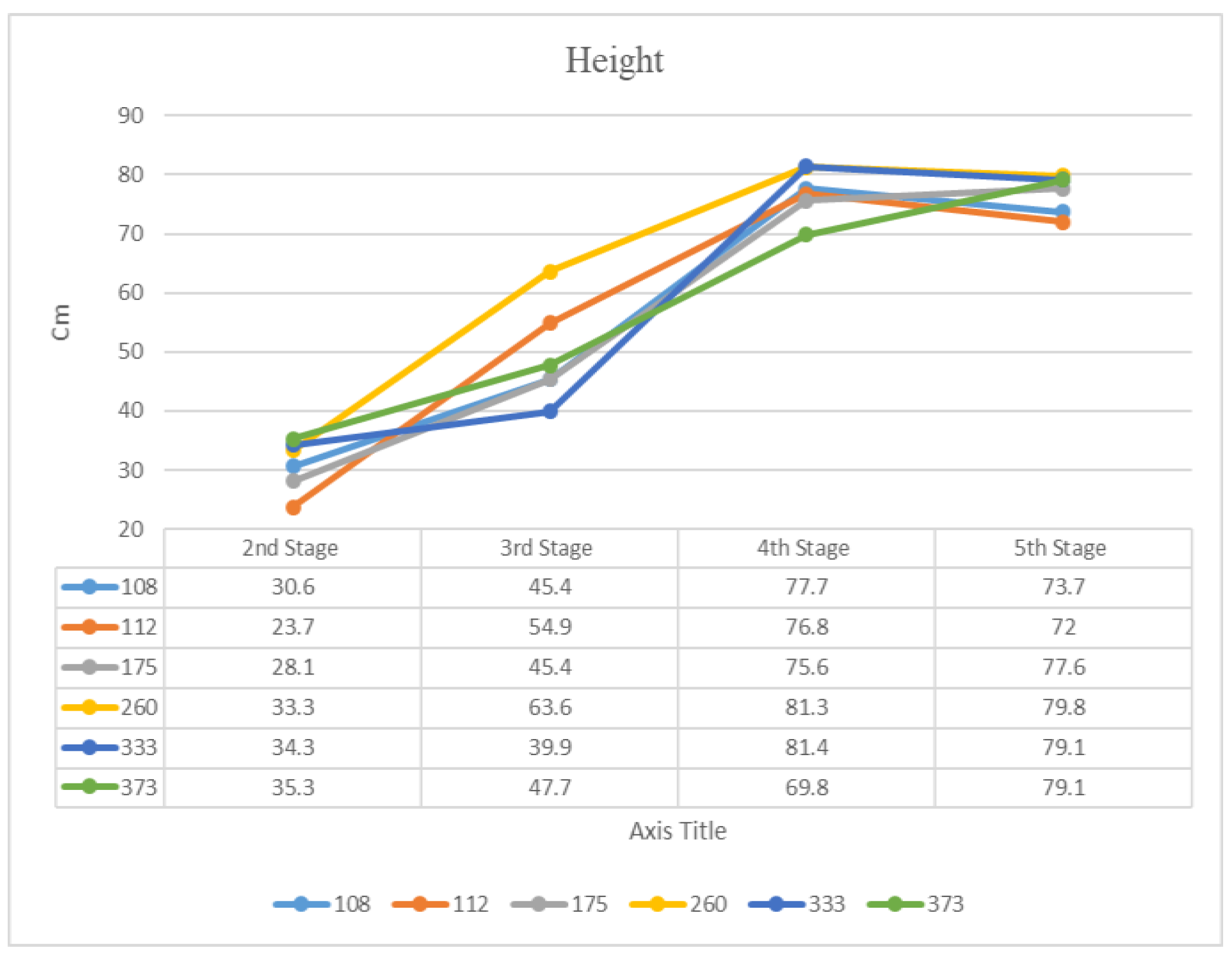
3.5. Analyzing Growth of Wheat Plots

In this section, plot #260 was selected randomly as a test plot to monitor growth of crop on this plot during the growing season of 2018.

Table 6. Variation of NDVI, height, temperature, ambient temperature/humidity values of plot #260 (selected randomly) during the growing season of 2018; collected by data acquisition module of Pheno-VISDM2 program.

Date	NDVI	Height (cm)	Canopy Temp (°C)	Ambient Temp (°C)	Ambient Humidity (%)
13 June 2018	N/A	35.1	30.9	31.2	56.2
26 July 2018	0.67	62.2	22.6	20.4	48.5
9 August 2018	0.37	78.8	28.4	27.2	41.8
23 August 2018	0.16	78.9	20.9	15.9	63.4

shows growth related data, and Figure 17 and Figure 18 illustrate the changes during different stages of wheat growth.

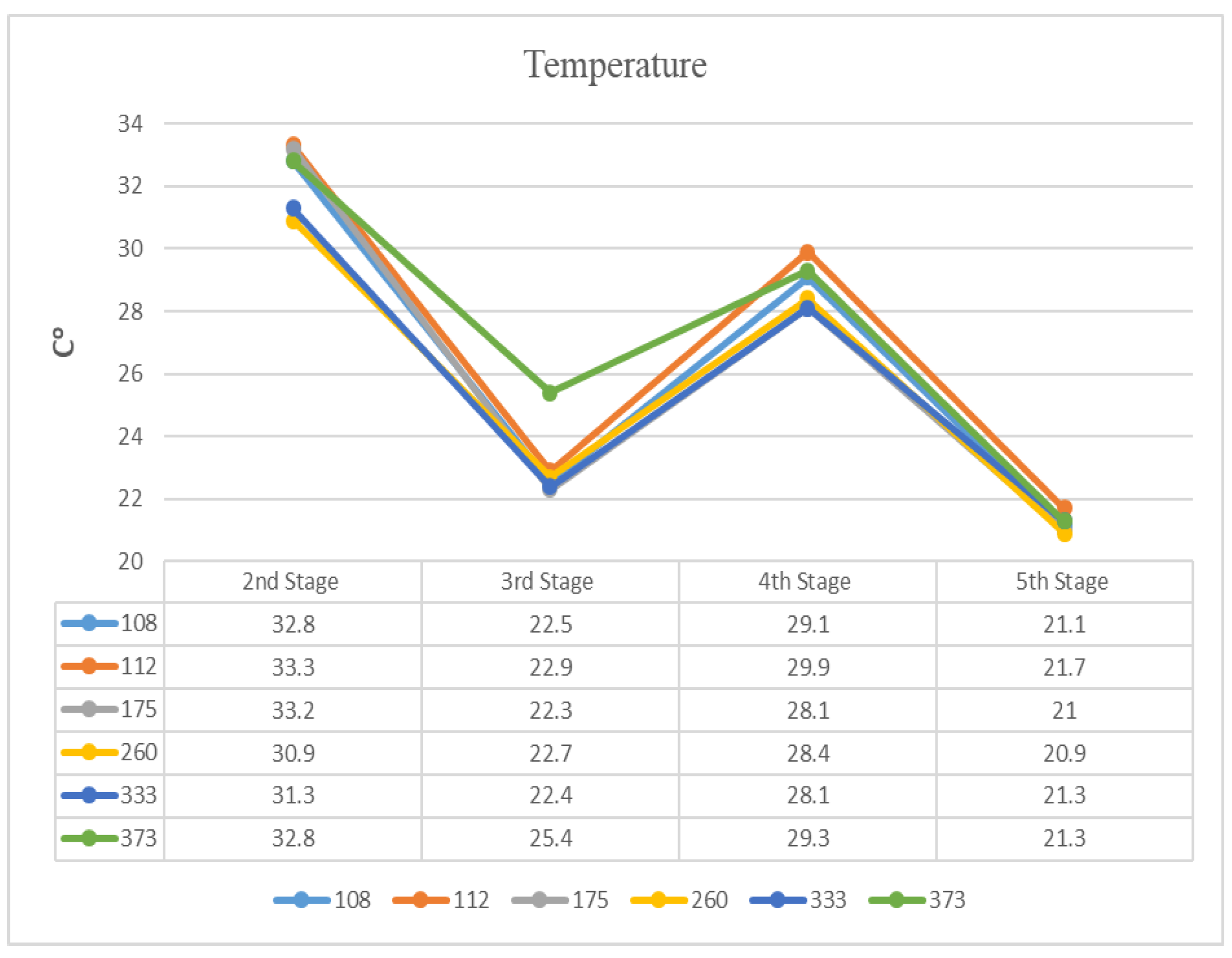
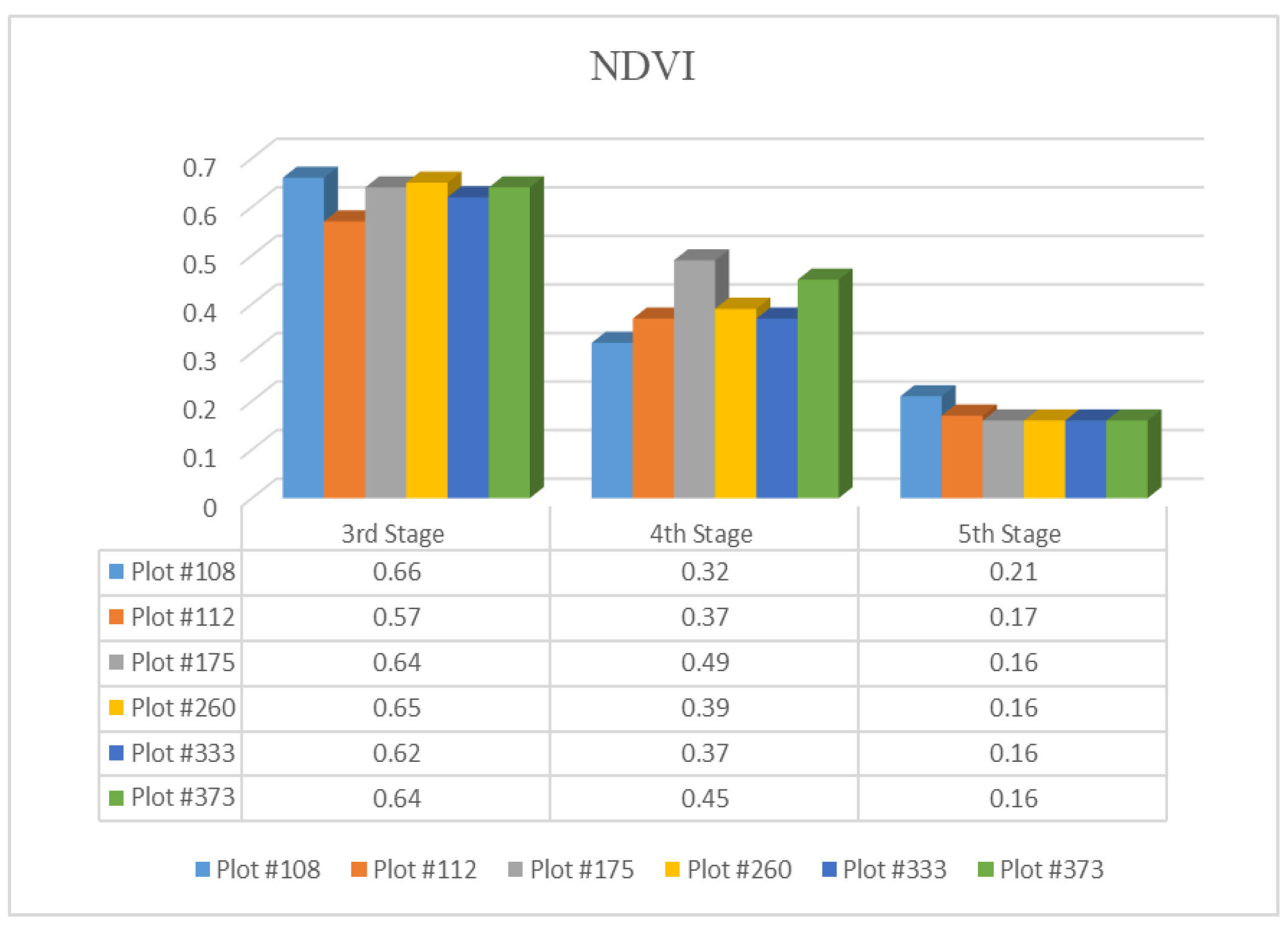
3.6. Comparing Traits of Different Genotypes of Wheat Plots

By use of Pheno-VISDM2 program, collected data and images were sorted, and valuable information was prepared for analysis. From each genotype, a random plot was selected, and the behaviors of selected plots were compared with each other, as can be seen in Figure 19, Figure 20 and Figure 21. By use of these diagrams and related information, the breeder can detect stronger gens and increase yield.

4. Discussion

Over the last 2 years, a mobile ground-based platform was developed for high-throughput phenotyping of several crops. In this study, we have focused on verifying the validity of the geo-referencing, accuracy of the height, and temperature measurements of wheat canopies, and analyzing the crop’s growth. The field experiments were done at a wheat breeding in Saskatchewan, Canada, facility that had 9 rows of crops with a total of 270 plots. The platform developed and results obtained in this study are satisfactory in comparison with previous reported works [6,7,8,9,10]. In [6,7,8], the platforms were not able to record all traits (height, temperature, vegetation index, and RGB images) simultaneously, while our platform is capable of doing so. In [9], two RTK-GPS systems were used for geo-referencing, while in our platform, we used only one RTX-GPS system with accurate results. In [10], the NDVI measurement method was passive and sensitive to sunlight and ambient conditions, while we used an active NDVI measurement system (digital) with almost no sensitivity to sunlight.

To verify the accuracy of developed HTPP and related programs, particularly geo-referencing and geo-tagging, 45 physical signs were placed next to different plots, randomly. The Pheno-VISDM2 Program brought up the right picture for four test days, 100% of time. It was found that the program is working very reliably, as this examination was continued for all other signs and each day of data collection. All physical signs matched with their corresponding location.

To analyze delay in the process of geo-tagging, $\Delta x$ and $\Delta y$ values were calculated and compared for several records, as discussed in Section 3.2. It can be concluded that they are almost equal and that recorded GPS data are valid and the process of geo-referencing is reliable.

As indicated in Table 5 (column 9 and 10), Diff and %Diff varied between −1.1 and −3.8 °C and −4% to −15%, respectively. The average Diff is −2.7 °C and average %Diff is 10%. The correlation between the manual measurements and the IRT sensor was found to be 0.6. Correlation values that are more than 0.5 and %Diff values that are less than 15% are acceptable in this research, as it is an acceptable norm among crop scientists. To have a more accurate temperature data, perhaps a thermal camera is a better option, which we have installed in our system recently. These values are acceptable and strong enough to conclude that the developed field based and mobile HTPP records temperature of plots reliably and accurately. Moreover, for height measurement, the correlation between method 1 (using four sensors) and manual height measurement was about 0.34, which is weak. The correlation between Method 2 (using five sensors) and manual height measurement was 0.8, which is very good. This correlation value is acceptable, and a few centimeters of difference in height measurements is unavoidable. Therefore, positive slope for regression line and strong correlation number are showing that using method 2 for height measurement is accurate and reliable.

As illustrated in Figure 17, canopy color changes from green to yellow, as expected. This corresponds well with NDVI (explained in the Section 2) measured using Crop Circle (see Figure 18a). These pictures and NDVI values were confirmed to be accurate by experts, i.e., crop scientist/breeder collaborators. Moreover, the accuracy of NDVI measurement is verified by use of a manual measuring device (Multispectral camera). Details of comparing NDVI values using Crop Circle and Multispectral camera will be reported in a future publication. Figure 18b shows increase of height, as expected, and the rate of increase is confirmed to be accurate. Figure 18c shows difference between ambient and canopy temperature, which again seems appropriate.

As can be seen in Figure 19, the genotype that is related to the plot 112 is under heat stress in the start of maturity stage (at 4th stage, it has maximum temperature 29.9 °C); this genotype needs more water than other genotypes. Moreover, from Figure 20, plot 333 has higher NDVI value in comparison with others at the end of maturity stage (at 5th stage, it has maximum NDVI value of 0.21). In other words, while other genotypes are in the latest stage of their growth and are ready for harvest, the genotype of the plot 333 needs more time to growth and be ready for harvest. As discussed, the higher value of NDVI means more greenness, and to harvest, this value should be low. Moreover, height of plots with different genotypes can be compared in different stages of growth, as can be seen in Figure 21. This comparison prepares valuable information for the breeders to detect strong and productive genotypes.

5. Conclusions

Results of monitoring for wheat crops in a breeding field, with about 270 plots are reported here. The mechatronic system developed and reported here can measure several traits, such as height, temperature, and NDVI, and can collect images (RGB and multispectral). The data and images were related (geo-referenced) to each plot using GPS-RTX information coming from the Tractor navigation system. Accuracy of geo-tagging of data was verified using experimental measurements. This constitutes an important research contribution aspect of our developed prototype. In addition, Pheno-VISDM2, software developed in house, is a valuable tool for data acquisition and analysis. Test runs of the system indicated the accuracy and reliability of our platform’s hardware and software. Moreover, accuracy of canopies’ height and temperature measurements were verified using several experiments. The platform can easily be used for monitoring other crops such as canola and peas. Mostly, height of the booms must be adjusted to use this platform for other crops. As a matter of fact, a slightly different version of this platform has been used for canola monitoring on a big canola field, around 3000 plots in 2020. Commercialization of our developed platform will likely be reality soon.

References

1. State of Food Security and Nutrition in the World 2019, Safeguarding against Economic Slowdowns and Downturns. Available online: https://www.unicef.org/media/55921/file/SOFI-2019-full-report.pdf (accessed on 12 April 2021).
2. FAO. How to Feed the World in 2050, Insights from an Expert Meet; FAO: Quebec City, QC, Canada, 2009; Available online: http://www.fao.org/wsfs/forum2050/wsfs-forum/en/ (accessed on 12 April 2021).
3. Furbank, R.T.; Tester, M. Phenomics—Technologies to relieve the phenotyping bottleneck. Trends Plant Sci. 2011, 16, 635–644. [Google Scholar] [CrossRef] [PubMed]
4. Cobb, J.N.; Declerck, G.; Greenberg, A.; Clark, R.; McCouch, S. Next-generation phenotyping: Requirements and strategies for enhancing our understanding of genotype–phenotype relationships and its relevance to crop improvement. Theor. Appl. Genet. 2013, 126, 867–887. [Google Scholar] [CrossRef] [PubMed] [Green Version]
5. Tisné, S.; Serrand, Y.; Bach, L.; Gilbault, E.; Ben Ameur, R.; Balasse, H.; Voisin, R.; Bouchez, D.; Durand-Tardif, M.; Guerche, P.; et al. Phenoscope: An automated large-scale phenotyping platform offering high spatial homogeneity. Plant J. 2013, 74, 534–544. [Google Scholar] [CrossRef] [PubMed]
6. Montes, J.; Technow, F.; Dhillon, B.; Mauch, F.; Melchinger, A. High-throughput non-destructive biomass determination during early plant development in maize under field conditions. Field Crop. Res. 2011, 121, 268–273. [Google Scholar] [CrossRef]
7. Fernandez, M.G.S.; Bao, Y.; Tang, L.; Schnable, P.S. A High-Throughput, Field-Based Phenotyping Technology for Tall Biomass Crops. Plant Physiol. 2017, 174, 2008–2022. [Google Scholar] [CrossRef] [PubMed] [Green Version]
8. Rischbeck, P.; Elsayed, S.; Mistele, B.; Barmeier, G.; Heil, K.; Schmidhalter, U. Data fusion of spectral, thermal and canopy height parameters for improved yield prediction of drought stressed spring barley. Eur. J. Agron. 2016, 78, 44–59. [Google Scholar] [CrossRef]
9. Barker, J.; Zhang, N.; Sharon, J.; Steeves, R.; Wang, X.; Wei, Y.; Poland, J. Development of a field-based high-throughput mobile phenotyping platform. Comput. Electron. Agric. 2016, 122, 74–85. [Google Scholar] [CrossRef] [Green Version]
10. Bai, G.; Ge, Y.; Hussain, W.; Baenziger, P.S.; Graef, G. A multi-sensor system for high throughput field phenotyping in soybean and wheat breeding. Comput. Electron. Agric. 2016, 128, 181–192. [Google Scholar] [CrossRef] [Green Version]
11. Bayati, M.; Fotouhi, R. A Mobile Robotic Platform for Crop Monitoring. Adv. Robot. Autom. 2018, 7, 186. [Google Scholar] [CrossRef]
12. Crippen, R. Calculating the vegetation index faster. Remote. Sens. Environ. 1990, 34, 71–73. [Google Scholar] [CrossRef]
13. Carballido, J.; Perez-Ruiz, M.; Emmi, L.; Agüera, J. Comparison of positional accuracy between rtk and rtx gnss based on the autonomous agricultural vehicles under field conditions. Appl. Eng. Agric. 2014, 30, 361–366. [Google Scholar]
14. Bayati, M. Development of a Field-Based Platform for Plant Phenotyping. Master’s Thesis, University of Saskatchewan, Saskatoon, SK, Canada, 2017. [Google Scholar]
15. Blogspot. Using Automator to get the absolute path of the selected file or folder in Finder in OS X 10.8.4. Available online: http://notinthemanual.blogspot.com/2008/07/convert-nmea-latitude-longitude-to.html (accessed on 18 May 2020).
16. Calculator Soup. Decimal Degrees to Degrees Minutes Seconds. Available online: https://www.calculatorsoup.com/calculators/conversions/convert-decimal-degrees-to-degrees-minutes-seconds.php (accessed on 18 May 2020).
17. Anisya; Swara, G.Y. Implementation of Haversine Formula and Best First Search Method in Searching of Tsunami Evacuation Route. Proc. IOP Conf. Ser. Earth Environ. Sci. 2017, 97, 012004. [Google Scholar] [CrossRef]
18. Gogtay, N.J.; Thatte, U.M. Principles of Correlation Analysis. J. Assoc. Phys. India 2017, 65, 78–81. [Google Scholar]
19. Smarandache, F. Alternatives to Pearson’s and Spearman’s Correlation Coefficients. SSRN Electron. J. 2016, 3 (Suppl. S09), 47–53. [Google Scholar] [CrossRef] [Green Version]
Figure 1. System’s electrical devices for data collections on a wheat field with five ultrasonic sensors, two infrared thermometers, an ambient temperature and humidity sensor, two Crop Circle sensors, two BRIO webcams, and two multispectral cameras.
Remotesensing 13 01560 g001
Figure 2. Schematic of developed High-Throughput Phenotyping Platform (HTPP) with utilized devices and their distances in the field; IRT, US and CC stand for Infra-Red Thermometer, Ultrasonic Sensor and Crop Circle, respectively.
Remotesensing 13 01560 g002
Figure 3. Projected area of measuring devices ((a)—Infra-red Thermometer and Ultrasonic Sensor, (b)—Crop Circle Sensor) vary by changing height of the mechanical boom; they can be calculated according to Equations (12) and (13).
Remotesensing 13 01560 g003
Figure 4. Mounted boom on a 6-feet Tractor with sensors, cameras, Data Logger, computer, and GPS receiver in two modes: (a) transportation and (b) expanded mode.
Remotesensing 13 01560 g004
Figure 5. The developed GUI for RGB image acquisition program; user can test cameras and select format of saving and resolution of webcams.
Remotesensing 13 01560 g005
Figure 6. A schematic to show automatic pause of image acquisition program during the data collection.
Remotesensing 13 01560 g006
Figure 7. The structure of Excel database to store phenotypic data; each row of this table (record) consists time, geospatial information, and sensors’ values.
Remotesensing 13 01560 g007
Figure 8. Screenshot of Visualization module of Pheno-VISDM2 buttons on right side with blue color and plots in center and on left side with green color—a target data point is showing geospatial information, vehicle’s speed/heading, height of boom, and ambient temperature/humidity.
Remotesensing 13 01560 g008
Figure 9. Calculating geospatial information point P2 based on the longitude and latitude values of point P1 and distance k between two points on spherical coordinates.
Remotesensing 13 01560 g009
Figure 10. Physical visible signs for verifying the validity of geo-referenced data on the Pheno-VISDM2 program for (a) plot #330 on July 13 and (b) plot #274 on 23 August 2018.
Remotesensing 13 01560 g010
Figure 11. A screenshot from visualization module of Pheno−VISDM2 program to measure distances of two points to analyze possibility of delay in the geo-referencing process.
Remotesensing 13 01560 g011
Figure 12. Examples for comparing calculated distances between two points (P1 and P2) based on the speed information ( Δ x ) and GPS data ( Δ y ) in different records.
Remotesensing 13 01560 g012
Figure 13. The spectrum of the correlation coefficient in the range of −1 to 1.
Remotesensing 13 01560 g013
Figure 14. Scatter diagram (including regression line) between handheld and infrared thermometers’ temperature measurements of different wheat plots on 9 August 2018.
Remotesensing 13 01560 g014
Figure 15. Comparison between manual and ultrasonic sensor height measurements of 28 different wheat plots using five sensors (method 2, Section 2.1).
Remotesensing 13 01560 g015
Figure 16. Scatter diagram (including regression line) between manual and ultrasonic height measurements of different wheat plots (method 2, Section 2.1).
Remotesensing 13 01560 g016
Figure 17. RGB pictures of plot #260 during the growing season of 2018 on (a) 13 July, (b) 26 July, (c) 9 August, and (d) 23 August 2018; captured by image acquisition module of Pheno-VISDM2 program.
Remotesensing 13 01560 g017
Figure 18. Growth data variation for (a) NDVI, (b) height, and (c) crop’s temperature and ambient temperature traits of plot #260 during the growing season of 2018.
Remotesensing 13 01560 g018
Figure 19. Comparison of different genotypes’ temperature variations during different stages of growth.
Remotesensing 13 01560 g019
Figure 20. Comparison of different genotypes’ NDVI variations during different stages of growth.
Remotesensing 13 01560 g020
Figure 21. Comparison of different genotypes’ height variations during different stages of growth.
Remotesensing 13 01560 g021