1. Introduction
The recovery of metals, specifically critical raw materials (CRMs) from mining residues (stockpiles and tailings) is a current concern of EU research activity [
1] and an essential reason to call them “mining residues” instead of stockpiles and tailings or in general mining wastes. Besides, the environmental aspects have caused a strong push for more effective managements of mining residues in many mining sites [
2]. The characterization of mining residues—necessary, for example, to construct and classify database or for environmental assessment or for materials recovery projects—is a difficult and challenging task for several reasons. First of all, the scarce availability of data: often there are not sufficient economic justifications for mining companies in sampling the stockpiles and landfills [
3,
4]. This is done just for checking the ore dressing process or when imposed by environmental legislation, and even when available, the quality of such sampling is often imprecise (with poor or missing georeferencing) [
5,
6].
Moreover, standard approach for resource characterization is based on a geostatistical modelling (an unbiased estimation with minimum error variance), which is possible when the materials of interest have a spatial distribution [
7]. However, the spatial distribution of metal concentrations (grades) in a mining residue (for example tailings from processing plant) is artificial, meaning that the natural spatial variability of materials (e.g., metals) in the deposit, is not obeyed inside residues. While ore bodies have smooth and natural variability, mining residuals are formed by a highly artificial component (piled material belongs to the different process and are daily stocked in small areas by trucks). This is due to the mining process and to the interval time of piling materials [
8]. In practice, the original variability of materials in a deposit changes due to the specific part of the deposit mined during a given time interval (for example, richer zone of the deposit as possible premier excavations); the excavation methods and volumes size of the ore extracted; the strong homogenization of ore process because of crushing and milling; the definition of new products as the waste (tailings) because of metal separation and on the tailings disposal method which defines the localization of the new product sent to the tailings. This produces an “artificial” space-time variability of mining residue materials. For these reasons, a different analysis accounting for this artificial spatial variability must be established. Addition to this artificial effect, the lack of samples and difficulties in sampling from mining residues is another reason why classical estimation methods, such as ordinary kriging, cannot be easily adapted for mining tailings [
9].
In this perspective, remote sensing technology, with its potential to provide consistent data in space and time, can assist the analyses and compensate for the scarce basic information available. Nowadays, large data sources based on Earth Observation (EO) data are available for mapping different environmental variables. In particular, data from satellite imaging sensors flying as part of the European Union’s Copernicus Earth observation program can be utilized for a wide range of applications in a variety of sectors including the urban area management, regional and local planning, forestry and fisheries, etc. Moreover, the continuity of data in time (with free access of data) gives the possibility of continuous land monitoring.
There are already a number of researches exploiting the advantages of remote sensing interaction with geostatistical techniques, to map different variables in mining resources, mining residues, and acid mine drainage, mainly on pollution and environmental aspects [
10,
11,
12,
13,
14]. The reason is the use of fast and accessible methods for preliminary analysis using remote sensing approaches. Since 1999, Ferrier [
15] worked on waste rock and tailings produced from mining activities, focusing on environmental pollutions of materials and trace elements of tailings using airborne mapping and high imaging spectrometer data. As another example, Choe et al. [
16] used the spectral reflectance variations associated with the presence of heavy metals in soils to characterize the distribution of areas affected by heavy metals.
In other applications, in order to improve any variable (or thematic) map accuracy and to validate results, the remote sensing and geostatistical methods are integrated, however, with smoothing effects on results [
17,
18]. To generate maps with finer resolution pixels, the Sequential Indicator Simulation (SIS) approaches can be used [
19]. SIS and estimation approaches can be used to integrate the uncertainty of remote sensing data and in situ samples, to identify their spatial cross-correlation and to evaluate the uncertainty from land cover classified remotely sensed imagery. The Indicator Simulation can approximate the probability, if a pixel at the fine resolution map belonged to a specific class [
20]. In high resolution hyperspectral imagery, by geostatistical filtering of noise and regional background, detection of small anomalies was attained. As an example, one-meter resolution data were used and validated with in situ samples from a mine tailings site, and results demonstrated a reasonable efficient approach for very complex landscape [
21].
To improve any type of map (for space variables) in remote sensing, while there is a need to deal with the interaction among multiple variables and spatial information from neighbor data, joint Sequential Co-Simulation (SCS) with satellite images can be used. Gertner et al. [
22] showed that the SCS could reproduce the spatial variability of different variables and the spatial correlation among them, in order to quantify the effect of variation from all the components on the prediction of the vegetation cover factor. In the joint SCS, a hierarchy of the dependent variables should be defined and a variable with the high correlation is the starting point of a co-simulation. Other attempts were done by other authors with different techniques, such as Multiple-Point Statistics approaches (MPS) with applications in subsurface modeling, remote sensing, climate modeling, and rainfall simulations with a training image adaption [
23,
24,
25,
26,
27].
The present work aims to propose an appropriate method to map the metal concentrations of a critical raw material (aluminum oxide) in a bauxite residue (BR) [
28]. The main novelty is the use of the geostatistical co-simulation method (turning band algorithm) for the first time in a complex application of mining residues (red mud from the process of alumina). Moreover, this method is for the first time integrated with remote sensing multispectral imagery for mining residues applications. As mentioned, one of the main challenges for the materials characterization in mining residues, is a high-concentration variability within a small area, as a consequence of the so-called artificial spatial structure [
29]. Moreover, a variety of reasons (limited economic benefits, ponds or muddy areas, not accessible parts of wastes, stability hazards, inhomogeneity of grain size, among others) make the sampling from mining residues difficult and cumbersome [
8,
9].
Hence, according to this artificial spatial variability, the new approach proposed in this work has been used. It consists in a combined use of remote sensing data and Conditional Co-simulation (CCS) to improve the classical estimation methods (as an example: ordinary kriging, co-kriging, etc.).
Using data from a bauxite mine in Greece, the proposed approach was tested for (I) the characterization of a critical raw material content and (II) a comparison between the common methods (estimation) and proposed model (simulation) aided by EO variables for metals concentration mapping. The application of this framework on mining residue is possible only by exploiting remote sensing information, due to the lack of detailed in-situ information and the existence of spatial correlation between metal concentration and pixel values from remote sensing data.
2. Methodology
EO can be an appropriate data source for the analysis of mining residuals. Specifically, the remote sensing multispectral images provided by the Copernicus services can be merged with the daily dumping data information, to both characterize mineral concentrations (metals, non-metals or CRMs) and monitor tailings area in time and space. There are different types of data available from the case study used in this research. Conditional co-simulation (CCS) using the turning band (TB) method [
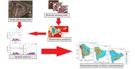
30] has been used for the first time in this work to check how it can improve the metals concentration maps accuracy in mining residues. Due to the presence of fourteen field samples (validation samples), there was the possibility of validating the simulation results. The number of validation samples was limited because of not accessible parts, humidity and trucks piling movements. Moreover, because of daily materials accumulation, sampling had to be done exactly at the date of available satellite image and this point made more limitation of in-field sampling. The proposed approach is presented in the flow sheet of
Figure 1, showing the methodology and remote sensing data and daily dumping data interaction for mapping.
The different contents of the building blocks are illustrated hereinafter. Firstly, after collection of the daily dumping data and relative Sentinel-2 images [
31], the basic statistical analysis (histograms) is performed (as the main variable). At the same time, within the Sentinel-2 images, the appropriate band ratios are calculated (as the auxiliary variable). Moreover, because of the randomly accumulation of materials by the Company, an unsupervised classification of the images is used to define homogenous areas as a guide to optimize the choice of the validation samples within the BR. One of the common methods for un-supervised classification is the K-means cluster analysis method [
32]. Then, based on the distribution of data, both (the main and the auxiliary variables) are transformation into Gaussian distribution to be ready for geostatistical analysis [
33]. As it is shown in the flow chart (see
Figure 1), the spatial analysis (direct and cross variograms) is performed on data and by the most consistent models, the CCS is tested. Fourteen validation samples are used to validate the results and better choosing the simulated concentration maps.
2.1. Remote Sensing Background
In multispectral solar wavelength remote sensing studies, different minerals in a target area (mainly in geological mapping), are often identified through the analysis of some band ratios [
34,
35]. Usually, they involve at least one band with higher reflectance features of the given material and another band with strong absorption features for the same material [
36]. There are many studies on spectral analysis of minerals based on different satellite images. One common tool, used for bauxite sources, is laterite band ratio [
37,
38,
39]. In this work, since the strategy of the project was using only free-access data, Sentinel-2 (Level-2, with atmospheric correction) images were selected for remote sensing analysis. Moreover, other band ratios were tested, but laterite band ratio (
Table 1) was selected as appropriate auxiliary variable for aluminum in this research.
The band ratio information, as it is an indirect measurement, is to be calibrated and validated with in situ samples to provide concentration estimates. The daily dumping data and the band ratio information can be combined for the estimation of the resource. This integration can be implemented in geostatistical modeling for mapping a spatial variable in an area with limited information. It has been shown by preceding studies [
40] that spectral signature analysis aids the identification of the appropriate bands and ratios. Besides, the key point for choosing the appropriate band ratio and its integration with daily dumping data, is the meaningful spatial correlation between samples and the band ratios derived from Sentinel-2 images. The spatial correlation is defined in Geostatistical background section.
2.2. Geostatistical Background
Geostatistical conditional simulation is used to predict complex variables (which depend on the regionalized variable at hand and need to consider a distribution compatible with the true one) and allows to quantify properties on which problems in different fields depend such as mineral resources evaluation, reservoir characterization, hydrology, soil, and environmental sciences [
41,
42,
43]. Geostatistical simulation allows the generation of different realizations of a regionalized variable that reproduce the original spatial variability over a field. In order to use the characteristics of spatial variability over the field, the experimental variograms (Equation (1)) need to be calculated for values of the target variable in space (with the distance h between samples) and fitted by a mathematical model [
44]. The fitted mathematical model quantifies the correlation between values as a function of the distance and demonstrates the continuity in average of regionalized variables.
where
γ(
h) is the experimental variogram (direct variogram for one variable) obtained from data values,
z(
x +
h) is a value at location
x +
h, while
z(
x) is a value at location x. There are a range of variogram models which can be used due to the variability behavior of target variable that can be found in almost all geostatistical references [
30,
45].
The standard geostatistical estimation is efficiently applied to natural variables, and simulation approaches mostly for local fluctuations. However, due to the artificial component of mining residues, testing the simulation approach can be suggested for mapping the concentration variability [
8], because of high variability of grades in small area and skipping the smoothing effect of estimation results.
Different methods and algorithms for simulation have been developed in the literature for modeling the regionalized variable or coregionalized variables (in the multivariate case) in Gaussian random fields with the spatial covariance of original variable [
46]. The turning bands (TB) algorithm, proposed by Matheron [
7], has the advantage of fast calculations and an accurate reproduction of the spatial correlation structure (in univariate and multivariate cases), even with distributions slightly different from the target ones [
47]. In the case of multi-variable, there is a need of cross-covariance functions to model the relationships between the main variable (the variable to be estimated or simulated) and the auxiliary variables (additional information and data) [
41]. Even in presence of medium correlation [
48], CK can be performed for verifying, by the analysis of the estimation variance, the effect of the secondary variable on estimation smoothing [
30]. Most of the geostatistical simulation methods rely on the (multi) gaussian framework, so data transformation from the raw to the gaussian space is needed. Afterwards, the posterior transformation of the gaussian simulated results to the raw scale is necessary. This transformation is called the gaussian anamorphosis and it includes different methodologies such as log-normal, Hermite polynomials, etc. An anamorphosis allows to reproduce the original distribution of the variable [
33]. In multivariate applications, some of simulation algorithms may be challenging and require simplifications [
49]. In the case of the TB, the method generates multi-dimensional simulations by 2D or 3D convolution of several random independent 1D simulations along lines with specific variogram models able to reproduce the true variogram (2D or 3D). The simulated values are obtained from the average of the projected values at the desired locations (e.g., the structured grid). To formulate the simulation, due to Matheron (1973), the true value of a variable at a location, is equal to its kriging estimated value, plus the kriging error (Equation (2)): The TB simulation estimates by kriging the values at grid nodes and adds the simulated estimation error [
30]:
where
Zk∗(
x) represents the kriging estimator of
Z(
x) at the point x based on the sample
Z(
x). The kriging error is unknown since
Z(
x) is not known. Considering the same equality for simulation,
S(
x), where
Sk∗(
x) is the kriging estimator, and the simulation is obtained only at the sample points (conditioned by samples) (see Equation (3)):
In Equation (3), the true value
S(
x) is known (we have samples) and so is the error
S(
x) −
Sk∗(
x). Hence, with substituting, the conditional simulation
Ycs (
x) of TB can be performed by two kriging parts and can be written as Equation (4):
Kriging at sample points is an exact interpolator, so at a sample location
Zk∗(
x) =
Z(
x) and the simulated error is zero:
Sk∗(
x) =
S(
x), so
Ycs(
x) =
Z(
x). Each realization (in a conditional simulation) shows a random result, that matches the sample points. Equivalently, it is a realization of a random function with a conditional spatial distribution [
30].
To validate the simulation results, and to choose the coherent map (between all simulation realizations), several methods can be applied [
30]:
Reproduction of the variogram model by the simulation results [
46]: it means that the reproduced variograms from simulation results should be coherent with the variogram model of the samples (the experimental variogram).
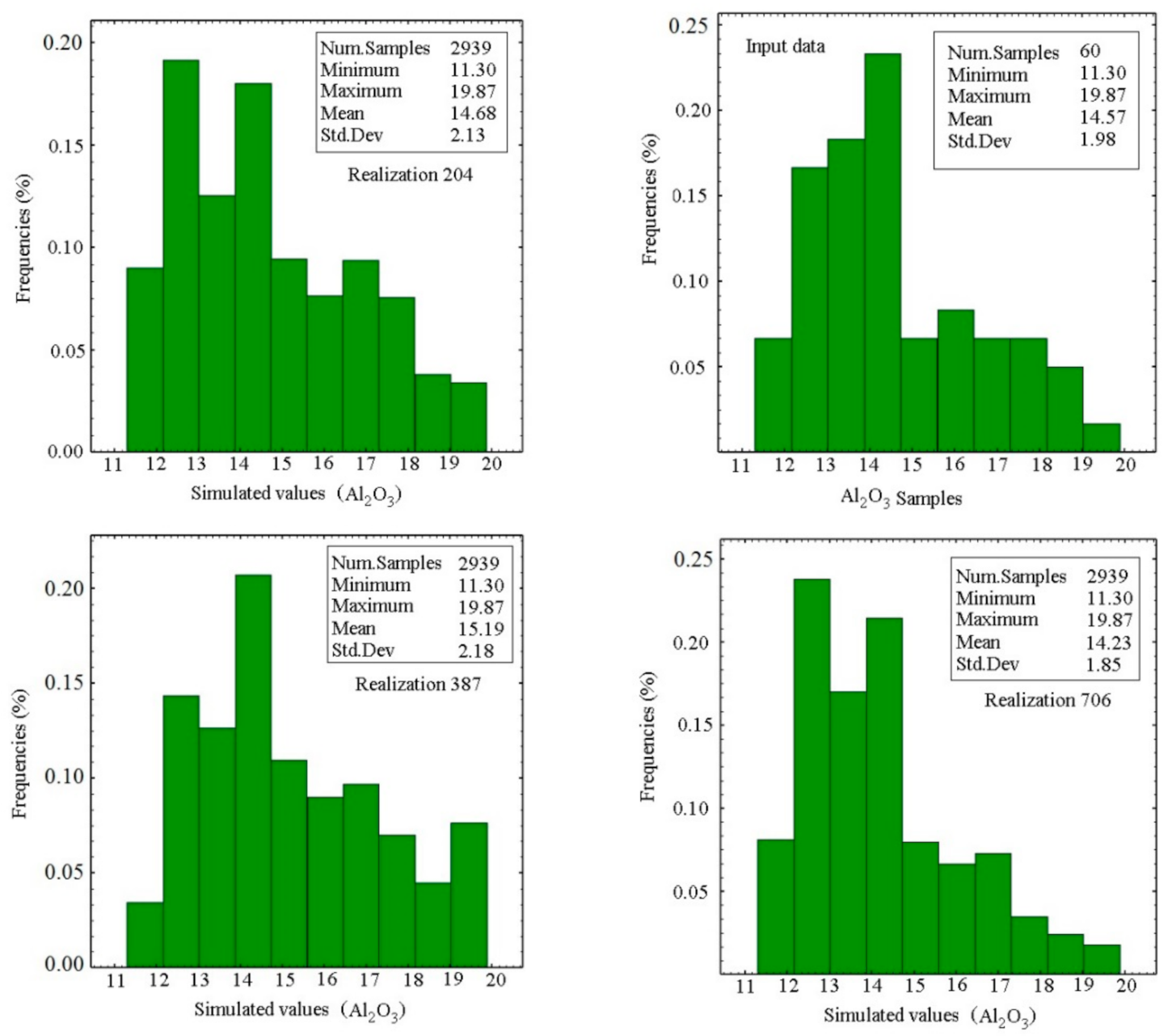
Matching the histogram: comparison of statistical parameters of simulation realizations with input data; the histogram match means the comparison between the histograms and statistical parameters of the simulation results with the histograms of input data. The simulation results with the highest correlation coefficients are the most acceptable realizations.
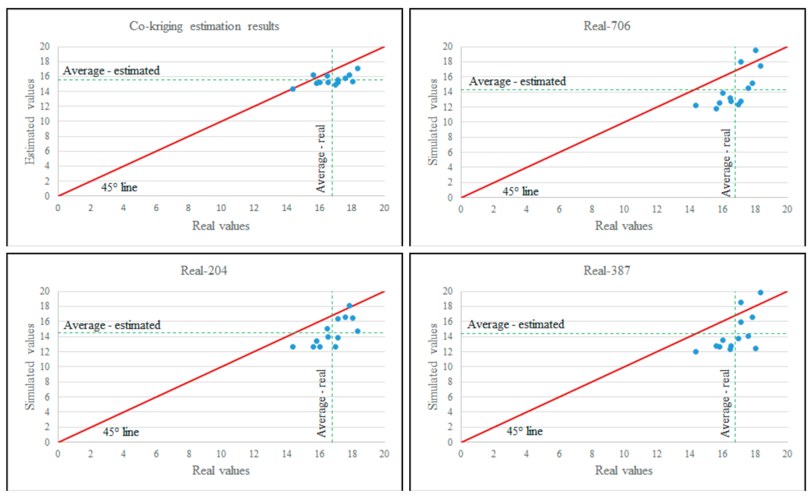
Validation of simulation results with real data (validation samples from the case study). The validation samples can be used to select the most accurate maps among all simulated realizations. After back transformation of simulation results, they can be compared with the validation sample values, and due to correlation parameters, the most accurate maps among all simulation realizations can be selected.
It is useful to compare conditionally simulated and estimated kriged models. Indeed, the characteristics of the simulated variable results should be similar to the kriged values but with larger dispersion, namely equal to the input data one. In this case study, the co-kriging estimation (using the same input data, variogram models and estimation parameters) as simulation is performed to do a comparison with simulation results. Moreover, to perform the anamorphosis, the hermit polynomial function was used to transform input data (daily dumping data and band ratios) into Gaussian field, because of the better fitting.
3. Study Area: Bauxite Residuals in Greece
The selected case study is an active BR site from the alumina refinery of Mytilineos S.A. in Greece. It is located on the Gulf of Corinth, 136 km from Athens (latitude 38.354177° and longitude 22.704671°, WGS84) with an area of around (700 m × 600 m). From 2006, a total of four filter presses were installed in the plant, to dewater the BR and since 2012 all BR produced is filter-pressed and stored as a “dry” (water content < 26%) by-product in an appropriate industrial landfill (see
Figure 2) [
50].
The dry stacking of the BR is the best technique for BR materials accumulating, because it significantly decreases the volume to be deposited, and it decreases the risk of dam failures [
49]. The BR, stored nearby the processing plant, contains a significant amount of raw materials which can be used for effective utilization. Different types of data were collected to characterize BR. Due to the analysis done on the BR, it has potential as a secondary resource for REEs extraction [
51], and TiO
2, V
2O
5, Al
2O
3, Fe
2O
3, CaO, Na
2O, and SiO
2 resources. The underlying target of this research is assessing the potential for recovering CRMs from BR of the selected case study. Hence, the characterization of Al
2O
3 concentrations within the BR (bauxite as CRM) was fundamental.
3.1. Daily Dumping Data
As a part of the standard management practices adopted by the mining company, daily information about piling operations is collected from the processing plant after performing filtering into piles. The daily dumping data include the tonnage of materials with their mean concentration value, and the area in which they were accumulated (Z, H, B, A, E, Γ, or ∆ in
Figure 3); however, the exact coordinates where trucks discharged the daily load of materials are not recorded. This lack is quite common while discharging materials in mining residues and it is not a peculiarity of this case study. Therefore, to use this information, each daily reported concentration, was considered as a point sample according to the piling direction and defined inside the recorded area of BR (each point is representative of one day due to the piling direction within the area of Z, H, B, A, E, Γ, or ∆). This step was performed in GIS as follows.
A topographic map [
52] was used as the base map to identify the seven piling areas (
Figure 3). After georeferencing, the map was inserted in a Geographic Information System (GIS) software to identify the sample locations; through monitoring, the daily piling procedures were tracked (see
Figure 3). Two months are considered the appropriate time interval to map the concentrations variability, because during a period of two months there is no over-layer material accumulations, and each layer, which can be mapped superficially by satellite images, can be approximately considered as the extension of materials that were piled during this period. Therefore, to map the Al
2O
3 variability within the BR, two periods of two months each were selected (March–April 2019 and then June–July 2019). As it can be seen in
Figure 3, in the first two sequential months (March–April), materials were accumulated on areas Z, H, E, A, Γ, and ∆, without any over layering. Then during June–July, materials were piled over Z, H, E, A, and ∆.
Overall, within two months, 60 daily dumping data were considered for mapping (see
Figure 3a samples of March–April and
Figure 3b samples of June–July).
To validate the approach proposed here, a dedicated field campaign was carried out on 30 July, and 14 samples were collected from the BR field, this time recording the position through GPS. These samples were analyzed (through X-ray Fluorescence analysis-XRF) to obtain the same concentration information provided by the daily dumping data (TiO
2, V
2O
5, Al
2O
3, Fe
2O
3, CaO, Na
2O, and SiO
2), and were used only to validate the results. Basic statistical parameters from daily dumping data were calculated for available elements (see
Table 2).
The statistical parameters of input data (daily dumping data) are important, since they should be used for comparison of histogram matching of simulation results.
3.2. Remote Sensing Data
In this research, Sentinel-2 imagery was used. Sentinel-2 mission orbit is sun-synchronous orbit with 98.62° inclination and the Mean Local Solar Time (MLST) at the descending node is 10:30 (a.m.). The multispectral Instrument (MIS) on board Sentinel-2 has been driven by the requirement for large swath high geometrical and spectral performance of the measurements. The MSI measures the Earth’s reflected radiance in 13 spectral bands from VNIR to SWIR (
Table 3) [
31].
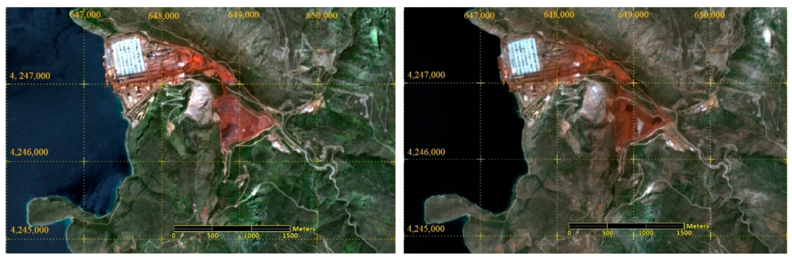
Coherently with available daily dumping data, two images were selected, one in the end of April (representing the period March–April 2019), and the second in July (representing the period June–July 2019). Level-2 atmospherically corrected spectral reflectance images were used:
S2B_MSIL_2A (30 July 2019), Processing level: Level 2A, and Sensing orbit direction: descending;
S2B_MSIL_2A (29 April 2019), Processing level: Level 2A, and Sensing orbit direction: descending.
The target zone in the presented images of
Figure 4 is the triangular area (reddish color) in the center of image, which shows the accumulated materials from the wastes of bauxite processing plant.
To map the Al2O3 concentration variability, the presented data (daily dumping data and Sentinel-2 images) were firstly analyzed separately, and then, by their integration, the spatial variability and geostatistical analysis were performed.
As a first step, the spectral patterns of BR surfaces extracted from the images were studied [
40]. All the Sentinel-2 bands were stacked and resampled at the 10 × 10 m spatial resolution. Resampling (Nearest Neighborhood method) is done because of different spatial resolution of bands (see
Table 3) in Sentinel-2 images. The spectrum analysis showed a certain variability within the BR deposits and some classes can be distinguished.
Figure 5 shows seven spectral patterns belonging to areas appearing spectrally different from photointerpretation. The selected seven classes are based on seven areas of materials accumulations (previously shown in
Figure 3 including Z, H, B, A, E, Γ, or ∆) that might have different material concentrations. The reason of the reflectance variability can result from several factors, such as, mineral grades, different humidity, or just being fresh or old materials.
A simple cluster analysis was performed to have a preliminary view of the piled materials before mapping the concentration variabilities. Since the spectral pattern analysis can explain the presence of different spectral clusters within the tailings, the un-supervised classifications were performed by K-means method [
32] with the assumption of seven classes. As explained before, the number of classes is based on the seven areas of materials accumulations (Z, H, B, A, E, Γ, and ∆ areas) that may present different physical or chemical properties, such as mineral composition, concentration, different humidity, or just being fresh or old materials (see
Figure 5). Results of the unsupervised classifications are reported in
Figure 6, where the seven classes are represented with different colors and with their relative frequency.
The unsupervised classification images were used only to check the tailings materials in different areas, and as a preliminary information to design the field sampling campaign for the validation of the final results.
To map the concentration variability of the Al
2O
3, the geostatistical Gaussian co-simulation using TB algorithm was used. The simulation is conditioned by daily dumping data (Al
2O
3 concentration data) but needs an auxiliary variable that is representative of the piling materials. Therefore, the laterite band ratio described in
Section 2.1 (see
Table 1) was computed from the Sentinel images (
Figure 7) and the correlation coefficient between selected band ratio (laterite band ration) and samples are shown in
Figure 7 (as example for data of June–July.
For verifying the use of image information, the spatial modelling of pile Al2O3 concentrations with band ratios was sought.
3.3. Spatial Analysis of Daily Dumping Data and Band Ratio
The spatial variability and the spatial correlation between laterite band ratio and daily dumping data were computed with the direct and the cross variograms. Direct variograms demonstrate the spatial variability of the main variable (Al
2O
3 grades of 60 daily data) and of the auxiliary variable (laterite band ratio), while the cross variogram identifies the spatial correlation between the Al
2O
3 grades and the laterite band ratio data (
Figure 8). The histograms, below each variogram, show the number of data pairs used for variogram calculations. Since the number of band ratios (2939 values equal to image pixels of BR) is much higher than 60 daily dumping data, the histograms of pairs have a higher number of pairs. The variogram models were composed of a nugget effect and two spherical structures (see
Table 4 for March and April 2019 and
Table 5 for June and July 2019) and called linear model of coregionalization [
41]. The total sills of direct variograms are close to 1 (0.85 for Al
2O
3 grade and 1.01 for laterite band in March–April variograms, and 1 for Al
2O
3 and 1.08 for laterite band in June–July).
The variogram behaviors suggest there is no specific trend in daily dumping data. Moreover, due to the selected ranges (maximum range is 180 m in
Table 4), locally stationary variograms are used. Therefore, spatial analysis does not need de-trending.
One thousand co-simulation of the Al2O3 concentration and with its band ratio was performed at nodes of a regular grid of 10 m × 10 m (equal to pixels resolution after resampling). TB method has been implemented conditioned by the 60 daily dumping data and the laterite band ratios as auxiliary variable using the presented variogram models.
5. Discussion
The use of free EO data, such as Sentinel images, can provide the missing information about the spatial variability of mineral grades, improving also the overall accuracy of the estimates. In this work, geostatistical conditional co-simulation using TB method was chosen for simulating CRM concentrations, to improve the variability map of aluminum. Sentinel-2 images provided a large amount of data that were used as auxiliary variable for the simulation.
The spatial analyses of selected variable (60 daily data and band ratio relating to aluminum concentration—Al2O3) were performed through direct and cross variograms. The direct variograms showed similar spatial behaviors during March–April and June–July (similar structures—Spherical—and similar ranges—between 160 and 180 m). In cross-variograms, both cases showed the negative spatial correlations. This confirms the similar spatial variability during the March–April and June–July time periods.
Results have proved the convergence of produced simulation variograms and their coherency with the experimental variogram of samples (see
Figure 9). The second step for validation of simulation results was carried out by using 14 in situ samples (validation samples) for BR, collected on 30 July 2019. The series of simulation results (1000 realizations) were checked with the validation samples; the best realizations (in terms of correlation parameters) were selected for mapping the Al
2O
3 concentration variabilities. The most coherent simulation was realization n° 204 with the correlation coefficient of 0.70 with validation samples. In addition to simulation, the geostatistical estimation method (Co-kriging) was used to estimate the Al
2O
3 variabilities in BR. Primary results (cross-validation of ordinary kriging with only daily dumping data and co-kriging using daily dumping and remote sensing data) proved that adding remote sensing data improves results with smaller estimation variance. In fact mapping only by the use of infield samples without EO data, could not reach to enough accuracy of estimation, while adding EO could improve the accuracy of concentration mapping. Results of estimation were compared with the selected simulation results. As it could be seen (in
Figure 12), the estimated maps show the smoothed concentration variations. However, since in mining residues the concentration variabilities are artificial (so there are high variations in small areas), in simulation maps, this sharp variability can be seen. Moreover, the simulation results were consistent with the estimation map.
The conditional co-simulation using TB method is an efficient method for mapping the metals variabilities within the BR and for evaluating the concentration variability of any possible mining residuals exploration and design. Remote sensing data have the potential to increase the accuracy and fill the gap of lacking in-situ samples, since it can supply a large amount of data. In Al
2O
3 concentration mapping, simulation realizations showed a higher correlation with validation samples, which approves the appropriate methodology used in this case-study. Hence, simulation results showed higher correlation with validation samples and might be considered as coherent maps for Al
2O
3 concentration variability. It is worthwhile to point out that the correlation of simulation results is also remarkably higher than the original correlation between the adopted band ratio and the mineral concentration of samples (
Figure 7); this proves the advantage of including a rigorous treatment of spatial correlation in remote sensing analyses. Finally, there are similarities between estimation map of the BR (rich areas on north-east and south-west), and the simulated maps (with realizations n° 204 and 706, but not in realization n° 387). The simulated map (realization n° 204), with the highest correlation can be considered as the most coherent map for Al
2O
3 concentration variabilities. The estimation map with smoothed results has the maximum similarity to this realization. To sum up, it can be noted that CCS is an appropriate method to characterize the sharp variability of metals within mining residues. However, the use of adequate validation samples is highly recommended. Besides, having the co-kriged map also will help to have a general view (smoothed) of concentrations variability. Further studies can be done for adding extra CRMs (such as vanadium) and check the possible spatial correlations. The proposed co-kriging methodology may result from new experiments on spatial cross-correlations, especially concerning the choice of the best auxiliary variables to be considered beside the existing ones. Moreover, it may be possible to include more than one auxiliary variable, if experimental results will justify it.


 ,
, 


