Feature Selection Based on Principal Component Regression for Underwater Source Localization by Deep Learning

Abstract

Underwater source localization is an important task, especially for real-time operation. Recently, machine learning methods have been combined with supervised learning schemes. This opens new possibilities for underwater source localization. However, in many real scenarios, the number of labeled datasets is insufficient for purely supervised learning, and the training time of a deep neural network can be huge. To mitigate the problem related to the low number of labeled datasets available, we propose a two-step framework for underwater source localization based on the semi-supervised learning scheme. The first step utilizes a convolutional autoencoder to extract the latent features from the whole available dataset. The second step performs source localization via an encoder multi-layer perceptron trained on a limited labeled portion of the dataset. To reduce the training time, an interpretable feature selection (FS) method based on principal component regression is proposed, which can extract important features for underwater source localization by only introducing the source location without other prior information. The proposed approach is validated on the public dataset SWellEx-96 Event S5. The results show that the framework has appealing accuracy and robustness on the unseen data, especially when the number of data used to train gradually decreases. After FS, not only the training stage has a 95% acceleration but the performance of the framework becomes more robust on the receiver-depth selection and more accurate when the number of labeled data used to train is extremely limited.

1. Introduction

Underwater source localization is a relevant and challenging task in underwater acoustics. The most popular method for source localization is matched-field processing (MFP) [1], which has inspired several works [2,3,4,5]. One of the major drawbacks of the MFP method is the need to compute many “replica” acoustic fields with different environmental parameters via numerical simulations based on the acoustic propagation model. Accuracy of the results is heavily affected by the amount of prior information about the marine environment (e.g., sound speed profile, geoacoustic parameters, etc.), which unfortunately is often hard to acquire in real scenarios.

Artificial intelligence (AI), and primarily data-driven approaches based on machine learning (ML), has become pervasive in many research fields [6,7]. ML-techniques are commonly divided into supervised and unsupervised learning. The former approach relies on the availability of labeled datasets, i.e., when measurements are paired with ground truth information. The latter refers to the case when unlabeled data are available [8].

Recently, there have been several studies on underwater source localization based on ML using the supervised learning scheme [9,10,11,12,13,14,15,16,17]. The general approach of underwater source localization by supervised learning scheme is through the use of acoustic propagation simulation models to create a huge simulation dataset for covering the real scenario. This approach has two main limitations: firstly, creating such a huge simulation dataset is time consuming and requires large computer storage resources; secondly, the set of environmental parameters to create a simulation dataset may not be able to account and adapt for environmental changes in a real-world scenario. The latter aspect requires a new simulation process, which may often be unrealistic.

Apparently, data-driven ML approaches rely on information extracted from available data, then the need of being able to exploit both labeled and unlabeled data is crucial in many applications, including underwater source localization. Semi-supervised learning has been proposed to face this issue in computer vision [18] and room acoustics [19,20].

Deep learning is famous for its brilliant performance for many tasks; however, the huge computation is the price. In the study of Niu et al. [15], the training time was six days for their ResNet50-1 model and three days for each of the ResNet50-2-x-D models. Each ResNet50-2-x-R model took 15 days to train.

In real scenarios, the speed of training is vital for real-time localization. To accelerate the training speed, some feature selection (FS) methods have been applied in underwater acoustics [21,22,23,24]. Feature selection aims to find the optimal feature subspace that can express the systematic structure of the raw dataset [21]. Principal component analysis (PCA) is a well-known method which can maximize the variance in each principal direction and remove the correlations among the features of the raw dataset [21,25]. Furthermore, the latent relationship between features can be interpreted by studying the correlation loading plot of PCA [26]. Principal component regression (PCR) is a PCA-based method, which can find out the significant variables for the target of regression by analyzing the absolute value of the regression coefficients [27,28].

In our study, an interpretable FS method for underwater source localization based on PCR is proposed. To make the situation closer to the real scenario, a two-step semi-supervised framework, and the data collected by a single hydrophone are used to build and train the neural network, respectively.

Figure 1 shows the workflow to illustrate our approach. The raw data is firstly preprocessed by discrete Fourier transform and min-max scaling. To select the important features for source localization, the PCR is conducted. Based on the absolute value of the regression coefficients of PCR, the important features are selected. Finally, the selected features are fed into the two-step semi-supervised framework for source localization. The structure of the framework is built on the encoder of a convolutional autoencoder which is trained in unsupervised-learning mode, and a 4-layer multi-layer perceptron (MLP) which is trained in supervised-learning mode.

The performance of our approach is assessed on the public dataset SWellEx-96 Event S5 [29].

The objectives of this paper are:

• Mitigating the problem related to the low number of labeled datasets in many real scenarios.
• Reducing the training time of the neural network and keeping the localization performance as much as possible.

More specifically, the contributions of our work are:

• An interpretable approach of FS for underwater acoustic source localization is proposed. This approach can reveal the important features related to sources by only introducing the source location without other prior information.
• By using the selected features, the training time of the neural networks is significantly reduced with a slight loss of the performance of localization.
• A semi-supervised two-step framework is used for underwater source localization exploiting both unlabeled and labeled data. The performance of the framework is assessed showing appealing behavior in terms of good performance combined with simple implementation and large flexibility.

The paper is organized as follows: Section 2 describes the theories of PCA and PCR, as well as the method of FS; Section 3 presents the two-step framework for underwater source localization; the public dataset SWellEx-96 Event S5, the data preprocessing, and the schemes of building the training and test datasets are given in Section 4; in Section 5, a comprehensive analysis of the localization performance between our framework based on the FS method and the control groups are described; the selected features are interpreted from both physical and data-science perspective in Section 6; and, finally, the conclusion is given in Section 7.

2. The Interpretable FS Method Based on PCR

The training time of a deep neural network could be huge, especially when the depth of the network is large. To reduce the training time, as well as keep the accuracy of the underwater source localization, an interpretable FS method based on PCR is introduced in this section.

2.1. Theory of PCA

PCA [28] refers to the following decomposition of a column-mean-centered data matrix $\mathit{X}$ of size $N\times K$, where N and K represent the number of samples and the number of features, respectively,

$$\mathit{X}={\mathit{T}\mathit{P}}^T+\mathit{E},$$

(1)

where ${(.)}^T$ is the transpose operation for a matrix, $\mathit{T}$ is a score matrix of size $N\times A$ related to the projections of the matrix $\mathit{X}$ into an A-dimensional space, $\mathit{P}$ is a loading matrix of size $K\times A$ related to the projections of the features into the A-dimensional space (with ${\mathit{P}}^T\mathit{P}=\mathit{I}$), and $\mathit{E}$ is a residual matrix of size $N\times K$.

More specifically, the A-dimensional space is identified via the singular value decomposition (SVD) of $\mathit{X}$ by selecting the first A principal components.

Denoting $\mathit{X}={\mathit{U}\mathit{S}\mathit{V}}^T$ the SVD of $\mathit{X}$ and $\widehat{\mathit{U}}$, $\widehat{\mathit{S}}$, and $\widehat{\mathit{V}}$ the matrices containing the first A columns of $\mathit{U}$, $\mathit{S}$, and $\mathit{V}$, respectively, then we have

$$\begin{array}{c}\hfill \mathit{T}=\widehat{\mathit{U}}\widehat{\mathit{S}}\\ \hfill \mathit{P}=\widehat{\mathit{V}}\end{array},$$

(2)

and $\widehat{\mathit{X}}={\mathit{T}\mathit{P}}^T$ is called the reconstructed data matrix.

2.2. Theory of PCR

The multiple linear regression (MLR) method is given by

$$\mathit{y}=\mathit{X}\theta +\mathit{e},$$

(3)

where $\mathit{y}$ is the regression target (in this paper is source location) of size $N\times 1$ containing N samples; $\mathit{X}$ is the data matrix as mentioned above; $\theta$ is the regression coefficients of size $K\times 1$; and $\mathit{e}$ is the unexplained residuals of $\mathit{y}$. Using ordinary least squares regression [30], the regression coefficients ${\widehat{\theta }}^{\mathrm{MLR}}$ of size $K\times 1$ can be estimated as

$${\widehat{\theta }}^{\mathrm{MLR}}={\left({\mathit{X}}^T\mathit{X}\right)}^{-1}{\mathit{X}}^T\mathit{y}.$$

(4)

PCR is the MLR based on the first A PCs extracted from the original data matrix $\mathit{X}$. To estimate the regression parameters ${\widehat{\theta }}^{\mathrm{PCR}}$ of size $A\times 1$, the score matrix $\mathit{T}$ is used instead of $\mathit{X}$ in Equation (4):

$${\widehat{\theta }}^{\mathrm{PCR}}={\left({\mathit{T}}^T\mathit{T}\right)}^{-1}{\mathit{T}}^T\mathit{y}.$$

(5)

2.3. Method of FS

The aim of FS is to select a set of important variables for accelerating the speed of underwater acoustic source localization. Furthermore, PCA and PCR are highly interpretable methods, the correlation between variables and the significant variables for regression can be revealed by investigating the plot of the correlation loading and the values of the regression coefficients, respectively [28].

The method of FS has 5 steps:

• Conducting mean-centered operation for each column in the data matrix $\mathit{X}$.
• Conducting SVD on the column-mean-centered data matrix $\mathit{X}$ to calculate the first A PCs ($A=3$ in this paper), as well as build the matrices of the score $\mathit{T}$ and the loading $\mathit{P}$, following Equation (2).
• Calculating the regression coefficients $\overline{\theta }$ of size $K\times 1$ for each original variable by

  $$\overline{\theta }=\mathit{P}{\widehat{\theta }}^{\mathrm{PCR}}.$$

  (6)
• Ranking the elements in $\overline{\theta }$ with absolute value from high to low. And setting a threshold $ϵ$ ($ϵ=0.02$ in this paper) to choose the variables equal to or greater than the threshold as the selected features.
• A new data matrix $\overline{\mathit{X}}$ of size $N\times M$ is constructed based on the selected M features.

3. The Two-Step Framework for Underwater Source Localization

In many real scenarios, a whole dataset will often consist of a small portion of labeled data and a large portion of unlabeled data (purely acoustic signals). To make the experiment condition closer to real scenarios, in the following, we assume that a large-size dataset is available with most of the data being unlabeled and only a small fraction labeled.

3.1. Step-One: Training a Convolutional Autoencoder

The autoencoder is an unsupervised learning machine, which can be trained based on the unlabeled dataset [31]. The first step of the framework is to train a convolutional autoencoder (CAE) [32]. The role of the CAE is to conduct unsupervised learning since training the CAE does not need labels, which means that the whole dataset can be covered.

The structure of CAE is shown in Figure 2a, where the network consists of an encoder and a decoder. The arrows indicate the direction of the data stream.

The encoder, made of 4 blocks, is used to extract the compressed features from the input data. Each block contains a convolution layer (for extracting features), a batch norm layer (for speeding up training), and a leaky-ReLU layer (for operating a non-linear transform on the data stream). Additionally, the decoder has a dual-symmetric structure as the encoder and is used to create the reconstruction of the input data from the compressed features. After creating the reconstructed input, the mean squared error (MSE) is the selected loss function to measure the difference between the input and the reconstruction.

It is worth noticing that, in this step, the whole dataset (both the labeled and unlabeled portions) is used to train the network, but only the purely acoustic signals are involved as described later in the paper.

3.2. Step-Two: Training the Encoder-MLP Localizer Based on the Semi-Supervised Learning Scheme

After training the CAE, the second step requires training the Encoder-MLP for localization based on the semi-supervised learning scheme. The structure of this model is shown in Figure 2b, which consists of a pre-trained encoder extracting the compressed features from input data and a 4-layer-MLP estimating the location of the acoustic source based on the compressed features. The MLP consists of four blocks, with each block containing a dense layer followed by a dropout layer (for regularization) and a non-linear transform function. The sigmoid function is an appropriate choice for the non-linear transform since, during the data preprocessing stage, the regression target, i.e., the horizontal distance between source and receiver, is scaled into the interval $(0,1)$.

Similarly, the arrows in Figure 2b indicate the direction of the data stream. Since the encoder has been trained, its parameters will be frozen during the training stage of the second step. After the encoder, the compressed features are fed in the MLP, which will provide the estimated source location as output. Finally, the same loss function, i.e., MSE, is used since the localization task is a regression problem.

4. Dataset and Preprocessing

In this section, SWellEx-96 Event S5 is introduced. The preprocessing method and the schemes for building the training and test datasets are used. Finally, to illustrate the performance of our framework and the proposed FS method, the control groups are created.

4.1. SWellEx-96 Event S5

Vertical linear array (VLA) data from SWellEx-96 Event S5 are used to illustrate the localization performance of our framework. The event was conducted near San Diego, CA, where the acoustic source started its track of all arrays and proceeded northward at a speed of 5 knots (2.5 m/s). The source had two sub-sources, a shallow one was at a depth of 9 m and a deep one at 54 m. The sampling rate of the data was 1500 Hz and the recording time of the data was 75 min. The VLA contained 21 receivers equally spaced between 94.125 m and 212.25 m. The water depth was 216.5 m. Additionally, the horizontal distance between the source and the VLA is also provided in the dataset. More detailed information of this event can be found in Reference [29].

4.2. Preprocessing and FS

In this paper, the underwater acoustic signals collected by a single receiver are transformed into the frequency domain. We calculate the spectrum without overlap for each 1 s slice of the signal and arrange it in a matrix (namely, features) $\mathit{X}$ format with the shape of $4500\times 750$, where each row is related to one slice. More specifically, 4500 is the total number of time-steps (75 min = 4500 s) and 750 is the number of frequencies. In the matrix, each row corresponds to one single time-step, and each column corresponds to one single frequency.

Besides the acoustic signals, the horizontal distance between the source and the VLA was provided in the original dataset, which can be expressed as a vector $\mathit{y}$ (namely, labels) with the shape of $4500\times 1$, where 4500 indicates the total number of time-steps, and 1 indicates the distance at each time-step.

For the training stability of our framework, the features $\mathit{X}$ and labels $\mathit{y}$ are scaled into interval $(0,1)$ by the min-max scaling method:

$$\begin{array}{c}\hfill \mathit{X}=\frac{\mathit{X}-{\mathit{X}}_{\min }}{{\mathit{X}}_{\max }-{\mathit{X}}_{\min }},\mathit{y}=\frac{\mathit{y}-{\mathit{y}}_{\min }}{{\mathit{y}}_{\max }-{\mathit{y}}_{\min }}.\end{array}$$

(7)

After preprocessing, the FS is conducted following the steps in Section 2 based on $\mathit{X}$ and $\mathit{y}$. Note that the systems with/without min-max scaling before FS have been compared showing that pre-scaling improves the performance.

4.3. Schemes for Building the Dataset

For step-one, the dataset for CAE is expressed as:

$$\left[\overline{\mathit{X}}\right]={\left[{\overline{\mathit{x}}}_i\right]}_{i=1}^N,$$

(8)

where $\overline{\mathit{X}}$ is the features in matrix form, ${\overline{\mathit{x}}}_i$ is a row-vector with the length of M (the number of selected features), corresponding to the ith row of the features matrix $\overline{\mathit{X}}$, and N is the number of time-steps.

For step-two, the dataset for Encoder-MLP localizer is expressed as:

$$[\overline{\mathit{X}},\mathit{y}]={[{\overline{\mathit{x}}}_i,y_i]}_{i=1}^N,$$

(9)

where $\overline{\mathit{X}}$ and $\mathit{y}$ are the features and labels in matrix form. And $y_i$ is the ith element in labels vector $\mathit{y}$.

4.4. Schemes of Separating Training and Test Datasets

To illustrate the performance of the semi-supervised framework as the number of labeled datasets decreases, 50%, 25%, and 12.5% of the whole labeled dataset are chosen, respectively, as the training dataset of step-two.

Since source localization is a regression task, the labels in the training dataset of step-two should cover the whole interval of the horizontal distance between the source and receiver. As described above, the total number of time-steps is 4500, which can be expressed by the index $i\in (1,4500)$. The schemes of separating training and test datasets for step-two are:

4.4.1. Using 50% Data to Build Training Dataset

$$\begin{array}{cccc}\hfill \mathrm{Training}\mathrm{dataset}& :({\overline{\mathit{x}}}_i,y_i)\hfill & \hfill & \forall i:mod(i,2)=1\hfill \\ \hfill \mathrm{Test}\mathrm{dataset}& :({\overline{\mathit{x}}}_i,y_i)\hfill & \hfill & \forall i:mod(i,2)\ne 1\hfill \end{array}.$$

(10)

4.4.2. Using 25% Data to Build Training Dataset

$$\begin{array}{cccc}\hfill \mathrm{Training}\mathrm{dataset}& :({\overline{\mathit{x}}}_i,y_i)\hfill & \hfill & \forall i:mod(i,4)=1\hfill \\ \hfill \mathrm{Test}\mathrm{dataset}& :({\overline{\mathit{x}}}_i,y_i)\hfill & \hfill & \forall i:mod(i,4)\ne 1\hfill \end{array}.$$

(11)

4.4.3. Using 12.5% Data to Build Training Dataset

$$\begin{array}{cccc}\hfill \mathrm{Training}\mathrm{dataset}& :({\overline{\mathit{x}}}_i,y_i)\hfill & \hfill & \forall i:mod(i,8)=1\hfill \\ \hfill \mathrm{Test}\mathrm{dataset}& :({\overline{\mathit{x}}}_i,y_i)\hfill & \hfill & \forall i:mod(i,8)\ne 1\hfill \end{array}.$$

(12)

To show the influence of different depths, receivers no. 1 (top), no. 10 (middle), and no. 21 (bottom) are chosen to build the dataset, respectively. For each receiver, there are 3 choices of the percentage to build the training dataset. Totally, there are $3\times 3=9$ training datasets are built.

4.5. Control Group

4.5.1. Control Group for the Semi-Supervised Framework

To make a fair comparison, we trained a neural network with the same structure as the framework by the purely supervised learning scheme.

4.5.2. Control Group for the FS Method

To show the performance of our FS method, a framework without FS is trained in the same way. The matrix containing the whole features $\mathit{X}$ of size $4500\times 750$ is calculated from Equation (7) and used to build the dataset following the schemes described in Section 4.3 and Section 4.4.

5. Performance of Source Localization

In this section, the hyperparameters of the two-step framework are introduced. After that, several experiments are conducted to exam the performance of source localization. Finally, a comprehensive comparison of the localization performance is shown, which demonstrates the benefit of our approach.

5.1. Hyperparameters of the Framework

In Figure 2, the output channel (n_Conv1D) and the kernel size (k_Conv1D) of the 1D-convolutional layer, as well as the input channel (n_Dense1) of the first dense layer, are not fixed. This is because the size of input features varies between datasets collected by different receivers.

For the training dataset without FS,

• n_Conv1D = 738;
• k_Conv1D = 13;
• n_Dense1 = 24,843.

For the training dataset with FS,

• n_Conv1D = 114;
• k_Conv1D = $M-113$;
• n_Dense1 = 507.

After FS, the number of selected features M is shown in

Table 1. Number of selected features among different receivers.

Receiver	50%	25%	12.5%
No. 1	121	122	125
No. 10	129	137	134
No. 21	126	126	127

.

To train the framework, the learning rates for step-one and step-two are 1 × 10${}^{-4}$ and 5 × 10${}^{-5}$, respectively. The optimization scheme is Adam. The epoch and the batch-size are 100 and 5 for each step, respectively.

All the networks mentioned in this paper are trained using one NVIDIA RTX 2080Ti GPU card.

5.2. Examining the Performance When Removing Some 2D-Convolutional Layers of the Framework after FS

The function of the encoder is to compress the original dataset and create its compressed expression, which is similar to our manual FS method. To find the best structure for the framework using FS, the number of 2D-convolutional layers of the encoder, and the corresponding number of transposed 2D-convolutional layers of the decoder are gradually decreased. After re-training the modified CAE, step-two is conducted as before. The structures of CAE after removing one and two 2D-convolutional layers are shown in

Table 2. Structure 1: Removing one 2D-convolutional layer of the encoder.

	Block	Output Channel	Kernel Size	Stride
	Conv1D	114	M-113	1
Encoder	Conv2D_1	128	$3\times 3$	2
	Conv2D_2	3	$3\times 3$	2
	Transposed-Conv2D_1	128	$4\times 4$	2
Decoder	Transposed-Conv2D_2	1	$4\times 4$	2
	Transposed-Conv1D	1	M-113	1

and

Table 3. Structure 2: Removing two 2D-convolutional layers of the encoder.

	Block	Output Channel	Kernel Size	Stride
Encoder	Conv1D	114	M-113	1
	Conv2D_1	3	$3\times 3$	2
Decoder	Transposed-Conv2D_1	1	$4\times 4$	2
	Transposed-Conv1D	1	M-113	1

, respectively. The performance will be discussed in Section 5.3.

5.3. Overall Analysis of the Localization Performance

To make a comprehensive comparison, 4 pairs of networks are tested on the data collected by all receivers and trained separately based on the data collected by receivers no. 1, no. 10, and no. 21. One pair is trained without FS, the rest are all trained with the FS method proposed by this paper. For the rest 3 pairs of networks, one has the same number of layers as the networks trained without FS; others have the structures shown in Table 2 and Table 3, respectively. Additionally, each pair of networks consists of the framework trained by the semi-supervised learning scheme and the same network of step-two trained by the purely supervised learning scheme.

5.3.1. Comparison between the Framework and the Purely Supervised Learning Scheme after FS

After FS and tested on all receivers, the performance of our framework and the purely supervised learning scheme is shown in

Table 4. The mean squared error (MSE) of models with feature selection (FS) trained on receiver no. 1.

	50%		25%		12.5%
	Framework	Supervised	Framework	Supervised	Framework	Supervised
R1	0.22	0.22	0.31	0.31	0.40	0.44
R2	0.31	0.33	0.36	0.39	0.48	0.51
R3	0.34	0.37	0.39	0.42	0.44	0.50
R4	0.35	0.39	0.43	0.44	0.45	0.55
R5	0.41	0.44	0.47	0.44	0.47	0.58
R6	0.39	0.42	0.4	0.42	0.42	0.54
R7	0.44	0.47	0.46	0.46	0.5	0.58
R8	0.38	0.4	0.38	0.43	0.42	0.48
R9	0.36	0.42	0.4	0.41	0.4	0.54
R10	0.39	0.43	0.46	0.45	0.48	0.59
R11	0.4	0.5	0.49	0.52	0.49	0.64
R12	0.39	0.4	0.43	0.46	0.46	0.54
R13	0.37	0.45	0.44	0.48	0.5	0.67
R14	0.4	0.49	0.49	0.49	0.49	0.63
R15	0.4	0.41	0.4	0.43	0.47	0.48
R16	0.47	0.49	0.48	0.5	0.56	0.59
R17	0.56	0.5	0.51	0.57	0.62	0.61
R18	0.43	0.47	0.45	0.51	0.51	0.57
R19	0.41	0.51	0.5	0.52	0.48	0.63
R20	0.43	0.51	0.51	0.53	0.53	0.67
R21	0.45	0.53	0.53	0.59	0.58	0.8
Mean	0.40	0.44	0.44	0.47	0.48	0.58

. In the Table, the first row indicates the percentage of the data used to build the training dataset. In the first column, R1 to R21 indicate receivers no. 1 to no. 21, respectively. Additionally, the mean indicates the average of MSE on all receivers. The bold numbers indicate the lower values of MSE in every pair of our framework and the purely supervised learning scheme, which means the model has a better performance on source localization.

Observing Table 4, interesting phenomena can be found:

• Performance of the purely supervised learning scheme:
  The network trained by the supervised learning scheme can attain the lower MSE only when the test dataset is chosen near the receiver used to build the training dataset. When the test dataset is far from the receiver used to train, its performance is getting worse dramatically. This trend is more obvious when the percentage of data used to train decreases. This shows the limitation of the purely supervised learning scheme: when the labeled training dataset is limited, the generalization ability of the model is poor.
• Performance of our framework:
  Compared to the purely supervised learning scheme, our framework is more robust and has much lower MSE on the data collected by those receivers which are far from the receiver used to build the training dataset, even though its performance on the data collected by the receivers near the receiver used to train is a bit poorer. This trend is more obvious when the percentage of data used to train decreases.
• Comparison of the different percentages used to train:
  When the percentage of the data used to build the training dataset decreases, the performance of both schemes becomes worse. However, the degree of performance degradation of our framework is smaller than that of the purely supervised learning scheme.

5.3.2. Comparison of the Mean MSE and the Training Time between the Networks with and without FS

The performance between the networks with and without FS is shown in

Table 5. Comparison of the mean MSE for networks with and without FS.

		Trained on R1		Trained on R10		Trained on R21
		Framework	Supervised	Framework	Supervised	Framework	Supervised
50%	Without FS	0.34	0.43	0.35	0.43	0.58	0.57
	With FS	0.40	0.44	0.41	0.48	0.48	0.49
	Residual	−0.06	−0.01	−0.06	−0.05	0.10	0.08
	Percentage of residual	−17.65%	−0.02%	−17.14%	−11.63%	17.24%	14.04%
25%	Without FS	0.39	0.57	0.40	0.52	0.66	0.79
	With FS	0.44	0.47	0.46	0.55	0.45	0.53
	Residual	−0.05	0.10	−0.06	−0.03	0.21	0.26
	Percentage of residual	−12.82%	17.54%	−15.00%	−5.77%	31.82%	32.91%
12.5%	Without FS	0.52	0.78	0.50	0.78	0.85	1.07
	With FS	0.48	0.58	0.52	0.58	0.47	0.53
	Residual	0.04	0.20	−0.02	0.20	0.38	0.54
	Percentage of residual	7.69%	25.64%	−4.00%	25.64%	44.71%	50.47%

. In the table, the residual illustrates the difference of the mean MSE between networks, and the percentage of the residual illustrates the performance improvement (positive value) and degradation (negative value) by FS. They are calculated by

$$\begin{array}{cc}\hfill & Residual=MS{E}_{WithoutFS}-MS{E}_{WithFS}\hfill \\ \hfill & PercentageofResidual=\frac{Residual}{MS{E}_{WithoutFS}}\hfill \end{array}.$$

(13)

Observing Table 5, phenomena can be found:

• When the percentage of data used to train is 50% and 25%, respectively, the performance of the framework trained on R1 and R10 has some degradation (12.82% to 17.65%). However, when the percentage of data used to train is 12.5%, the performance of the framework trained on R1 and R10 has a slight improvement (7.69%) and degradation (4%), respectively.
• Trained on R21, the framework’s performance has significant improvements, which are 17.24%, 31.82%, and 44.71% when the percentage of data used to train is 50%, 25%, and 12.5%, respectively.
• Compared to the framework, the performance of the purely supervised learning scheme gains more improvement (14.04% to 50.47%) after FS. The performance degradation only happens when it is trained on 50% R1, 50% R10, and 25% R10.

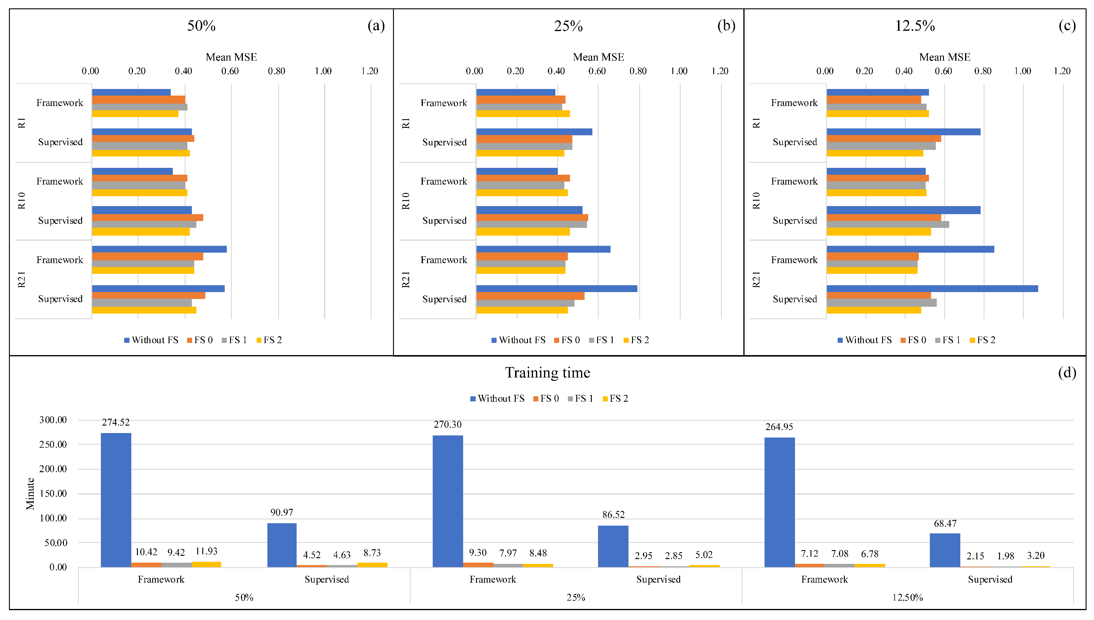
The training time of the networks is shown in

Table 6. Comparison of the training time for networks with and without FS.

		50%		25%		12.5%
		Framework	Supervised	Framework	Supervised	Framework	Supervised
Stet-one	Without FS	3 h 30 m 45 s	-	3 h 30 m 45s	-	3 h 30 m 45 s	-
	With FS	7 m 7 s	-	6 m 59s	-	7 m 4 s	-
	Percentage of reduction	96.62%	-	96.68%	-	96.65%	-
Step-two	Without FS	1 h 3 m 46 s	1 h 30 m 58 s	59 m 33 s	1 h 26 m 31 s	54 m 12 s	1 h 8 m 28 s
	With FS	3 m 18 s	4 m 31 s	2 m 19 s	2 m 57 s	1 m 50 s	2 m 9 s
	Percentage of reduction	94.82%	95.03%	96.11%	96.59%	96.62%	96.86%

. This table illustrates that the training time is reduced significantly after FS for both framework and the purely supervised learning scheme.

5.3.3. The Best Structure for the Framework after the FS

As mentioned in Section 5.2, the comparison of the mean MSE and the training time between different structures of networks is shown in

Table 7. Comparison of the mean MSE for different structures of the networks after FS.

		Trained on R1		Trained on R10		Trained on R21
		Framework	Supervised	Framework	Supervised	Framework	Supervised
50%	Original structure	0.40	0.44	0.41	0.48	0.48	0.49
	Structure 1	0.41	0.41	0.40	0.45	0.44	0.43
	Structure 2	0.37	0.42	0.41	0.42	0.44	0.45
25%	Original structure	0.44	0.47	0.46	0.55	0.45	0.53
	Structure 1	0.42	0.47	0.43	0.54	0.44	0.48
	Structure 2	0.46	0.43	0.45	0.46	0.44	0.45
12.5%	Original structure	0.48	0.58	0.52	0.58	0.47	0.53
	Structure 1	0.51	0.55	0.50	0.62	0.46	0.56
	Structure 2	0.52	0.49	0.51	0.53	0.46	0.48

and

Table 8. Comparison of the training time for different structures of the networks after FS.

		50%		25%		12.5%
		Framework	Supervised	Framework	Supervised	Framework	Supervised
Step-one	Original structure	7 m 7 s	-	6 m 59 s	-	7 m 4 s	-
	Structure 1	5 m 27 s	-	5 m 27 s	-	5 m 17 s	-
	Structure 2	3 m 42 s	-	3 m 42 s	-	3 m 44 s	-
Step-two	Original structure	3 m 18 s	4 m 31 s	2 m 19 s	2 m 57 s	1 m 50 s	2 m 9 s
	Structure 1	3 m 58 s	4 m 38 s	2 m 31 s	2 m 51 s	1 m 48 s	1 m 59 s
	Structure 2	8 m 14 s	8 m 44 s	4 m 47 s	5 m 1 s	3 m 3 s	3 m 12 s
Total	Original structure	10 m 25 s	4 m 31 s	9 m 18 s	2 m 57 s	8 m 54 s	2 m 9 s
	Structure 1	9 m 25 s	4 m 38 s	7 m 58 s	2 m 51 s	7 m 5 s	1 m 59 s
	Structure 2	11 m 56 s	8 m 44 s	8 m 29 s	5 m 1 s	6 m 47 s	3 m 12 s

, respectively.

According to the Tables, interesting phenomena can be found:

• For the framework, Structure 1 attains the lowest MSE except for trained on 50% R1 and 12.5% R1.
• For the purely supervised learning scheme, Structure 2 attains the lowest MSE with a slight improvement compared to Structure 1 when the percentages of data used to train are 25% and 12.5%.
• Structure 1 shows the best performance for training time reduction. Considering both MSE and training time, the best structure after the FS is Structure 1.

5.3.4. Conclusions of the Performance Analysis

In Figure 3, the conclusion of the performance analysis is illustrated. The legend used in all the sub-figures is the same. The blue bar is related to the network without FS. The orange, yellow, and gray bars are related to the ’Original structure’, ’Structure 1’, and ’Structure 2’ in Table 7 and Table 8, respectively.

From Figure 3, interesting phenomena can be found:

• When the number of labeled data is gradually decreasing, the power of the framework with the semi-supervised learning scheme is revealed.
• The FS method is beneficial for both the framework and the purely supervised learning scheme, which can significantly decrease the training time with a slight loss of the performance of localization.
• After FS, the difference in performance between different receiver-depth is not significant, which means it can increase the robustness of the receiver-depth selection.

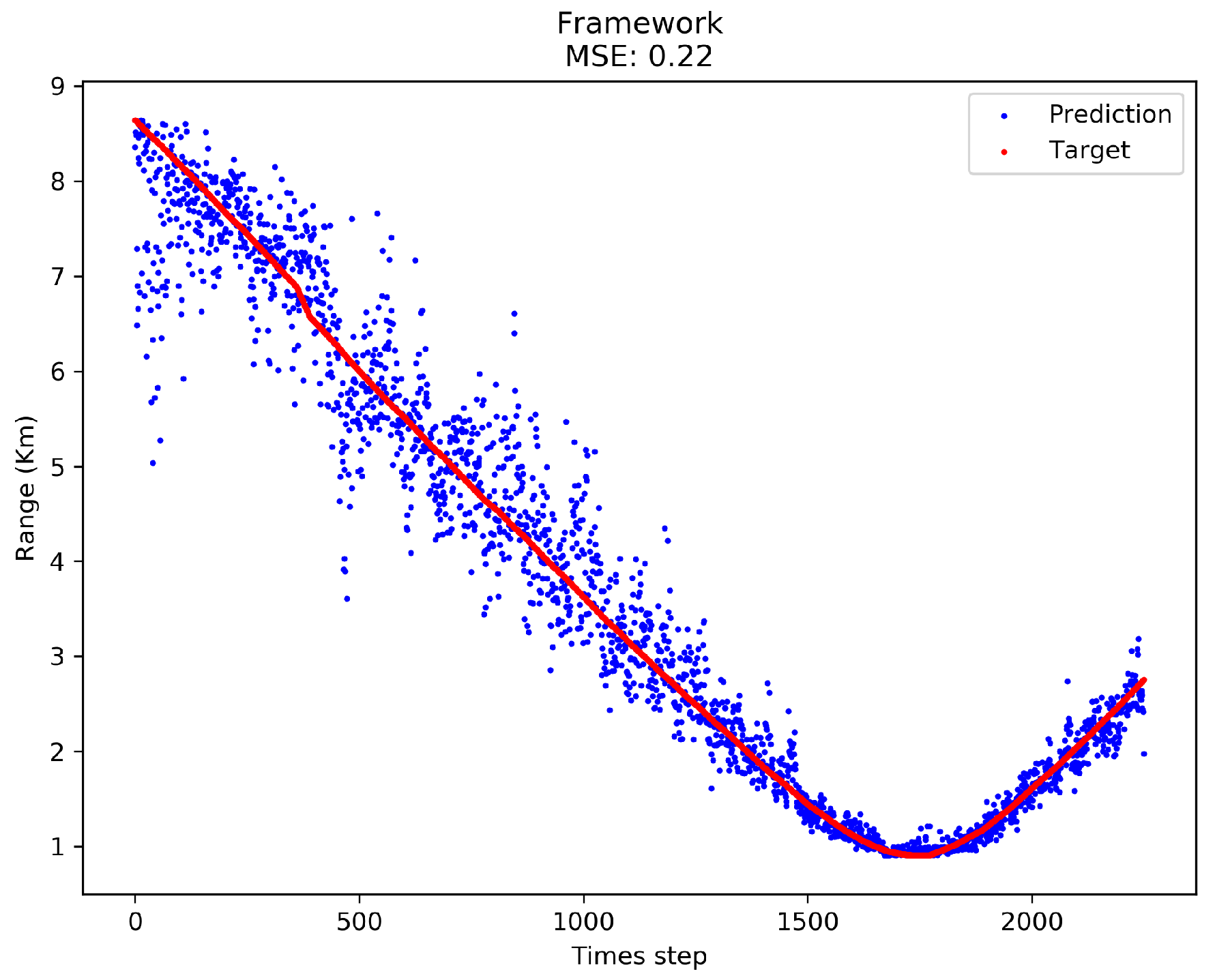
To have an intuitive view of the performance, Figure 4 shows the localization result of our framework trained on 50% R1 after FS.

6. Discussion of FS

In this section, the discussion of the selected features is given, which demonstrates that the most significant portion of the original features for source localization has been selected by performing the FS. The training dataset using 50% data collected by receiver no. 21 is used in this section for illustration.

6.1. Details of the Sources in SWellEx-96 Event S5

According to the details on the website of SWellEx-96 Event S5 [29], the deep source (J-15) transmitted 5 sets of 13 tones between 49 Hz and 400 Hz. The first set of tones was projected at maximum transmitted levels of 158 dB. The second set of tones was projected with levels of 132 dB. The subsequent sets (3rd, 4th, and 5th) were each projected 4 dB down from the previous set. The shallow source transmitted only one set containing 9 tones between 109 Hz and 385 Hz. According to Du et al. [33], 500–700 Hz is related to the noise radiated by the ship towing the sources in the experiment, which is also an important contribution for source localization.

6.2. Interpretation of the Selected Features

After the FS described in Section 2.3, the matrix $\overline{\mathit{X}}$ of size $N\times M$ containing selected features is created. To interpret the selected features, another PCA is conducted on this matrix. To investigate the correlation structure between the features and the PCs, correlation loading is calculated based on the method proposed by Frank Westad et al. [26].

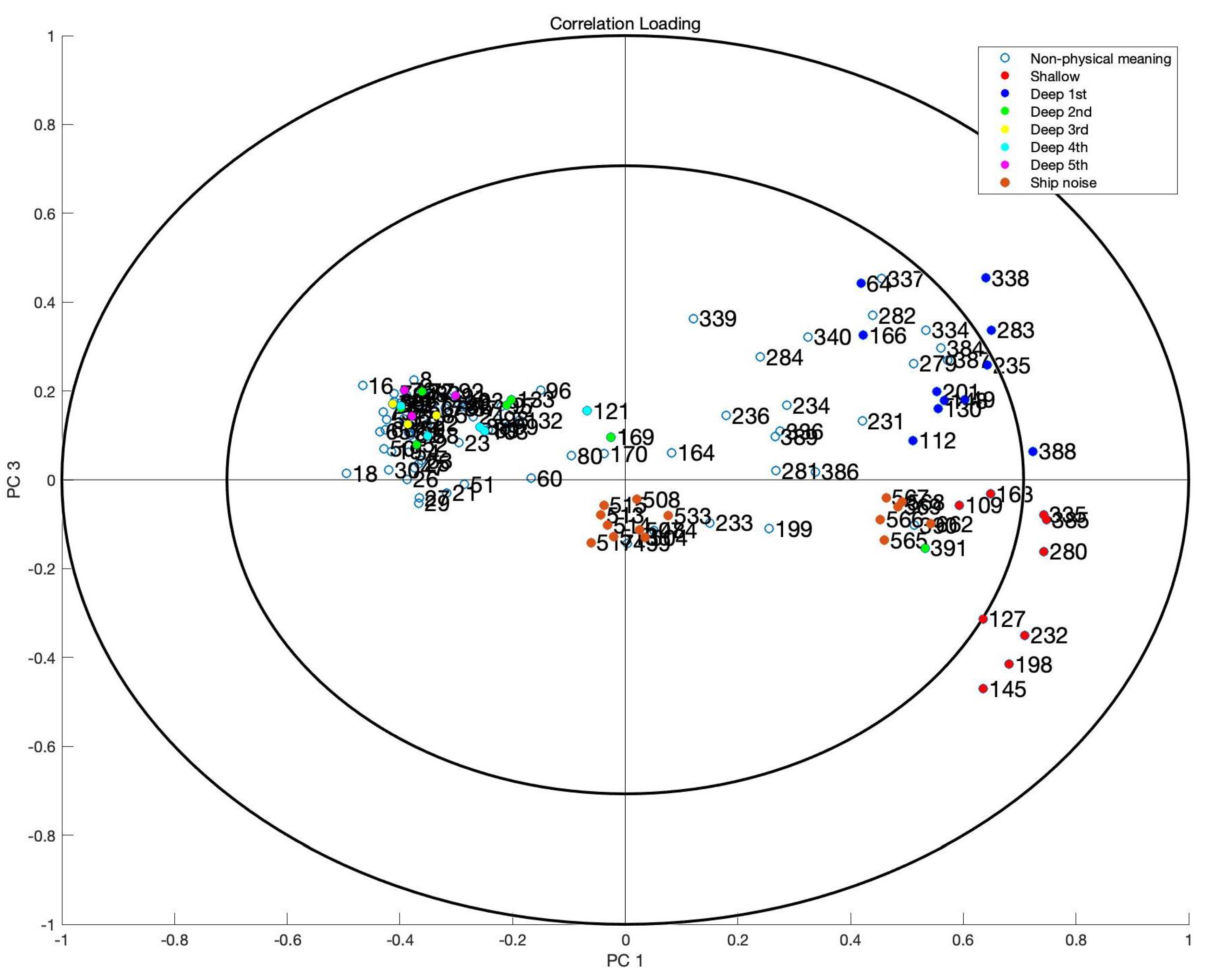
As shown in Figure 5, the abscissa is PC 1 and the ordinate is PC 3. There are 2 circles in the plot, in which the inner and outer ones indicate 50% and 100% explained variance, respectively. The points between the two circles are the significant features that can explain at least a 50% variance of the data. And the legend with different colors illustrates different sets of tones and the ship noise.

From the correlation loading plot in Figure 5, phenomena with physical meanings can be found:

1. Along PC 1, the frequencies related to the high transmitted signal level are in the positive half-axis. The frequencies related to lower energy levels are in the negative half-axis. For more details:

• 7 frequencies (127, 145, 198, 232, 280, 335, 385 Hz) of the shallow source and 3 frequencies (238, 338, 388 Hz) of the deep source are in the area between two circles, which means that they are significant features.
• The rest frequencies of the shallow source and the highest transmitted level (and also the tone with 391 Hz related to the second transmitted level) of the deep source are also close to the boundary of the inner circle, which means that they still have some importance for the data.
• Expect for frequencies of the highest transmitted level and 391 Hz of the second transmitted level, the rest frequencies are closer to the origin, which means that they are less significant from the statistical perspective.

2. Along PC 3, the frequencies related to the shallow source are in the negative half-axis (except for the tone with 391 Hz). Furthermore, the frequencies related to the ship noise are also in the negative half-axis, since the ship can be treated as a shallow noise source. The frequencies related to the deep source are in the positive half-axis.

More specifically, the numbers of selected features among the different subsets of tones and ship noise are:

• Deep 1st: 11 (13 in total);
• Deep 2nd: 7 (13 in total);
• Deep 3rd: 3 (13 in total);
• Deep 4st: 5 (13 in total);
• Deep 5st: 3 (13 in total);
• Shallow: 9 (9 in total);
• Ship noise (500–700 Hz): 15.

According to the discussion above, the frequencies related to the shallow source, deep source, and the ship noise are selected by applying the FS, which are the most important features for source localization. The FS process does not need any prior information.

6.3. Different Roles of the FS and the Autoencoder

Autoencoders are often used as feature extractors; thus, the considered feature-selection stage might seem redundant. However, the PCR adapted for FS is a linear method that can select the most important subset of variables for the regression target (i.e., source localization in this paper). The effect is that the non-linear processing of the autoencoder becomes easier to train (i.e., significantly reduced training time) while keeping approximately the same performance.

After the FS stage, the most important subset of the original features is gained.

More specifically, the roles of the FS and the autoencoder in our framework are:

• The FS: Selecting the most important subset of the original features for reducing the training time of our framework and providing a nice starting point for the framework.
• The autoencoder: Conducting the unsupervised learning to cover all the information in the dataset.

7. Conclusions

In this paper, we utilize a two-step semi-supervised framework for source localization to deal with the condition of the limited amount of labeled data in many real scenarios. To accelerate the training stage of the framework for the real-time operation, a FS method based on PCR is proposed.

Based on a public dataset, SWellEx-96 Event S5, the performances of our FS method and the two-step framework have been demonstrated. The results show that the framework is more robust on the unseen data, especially when the number of labeled data used to train gradually decreases. After FS, the training time is significantly reduced (by an average of 95%). The localization performance has a slight degradation when 50% and 25% of data are used to train. However, when the percentage of data used to train is 12.5%, this condition is closer to the real scenario, the FS method can improve the performance of both semi-supervised learning and purely supervised learning.

It needs to be mentioned that the structure of the network used in this paper is just a demo for showing the performance of our framework. More complex and powerful networks can be applied in this framework, and, based on our anticipation, the performance of source localization will be better as long as the network has been trained appropriately and well.