Article

Determining Peak Altitude on Maps, Books and Cartographic Materials: Multidisciplinary Implications

1
Department of Integrated Geodesy and Cartography, AGH University of Science and Technology, 30-059 Crakow, Poland
2
Department of Tourism and Regional Studies, Institute of Geography, Pedagogical University of Cracow, 30-084 Cracow, Poland
3
Center for Tourism Research, Wakayama University, Wakayama-City 640-8510, Japan
4
Faculty of Regional Development and International Studies, Mendel University in Brno, 613 00 Brno, Czech Republic
5
Faculty of Geography and Regional Studies, University of Warsaw, 00-927 Warsaw, Poland
*
Author to whom correspondence should be addressed.
Remote Sens. 2021, 13(6), 1111; https://doi.org/10.3390/rs13061111
Submission received: 15 February 2021 / Revised: 8 March 2021 / Accepted: 11 March 2021 / Published: 15 March 2021

Abstract

:
Mountain peaks and their altitude have been of interest to researchers across disciplines. Measurement methods and techniques have changed and developed over the years, leading to more accurate measurements and, consequently, more accurate determination of peak altitudes. This research transpired due to the frequency of misstatements found in existing sources including books, maps, guidebooks and the Internet. Such inaccuracies have the potential to create controversy, especially among peak-baggers in pursuit of climbing the highest summits. The Polish Sudetes Mountains were selected for this study; 24 summits in the 14 mesoregions were measured. Measurements were obtained employing the global navigation satellite system (GNSS) and light detection and ranging (LiDAR), both modern and highly precise techniques. Moreover, to determine the accuracy of measurements, several of the summits were measured using a mobile phone as an additional method. We compare GNSS vs. LiDAR and verify the level of confidence of peak heights obtained by automatic methods from LiDAR data alone. The GNSS receiver results showed a discrepancy of approximately 10 m compared with other information sources examined. Findings indicate that the heights of peaks presented in cartographic materials are inaccurate, especially in lesser-known mountain ranges. Furthermore, among all the mountain ranges examined, the results demonstrated that five of the summits were no longer classed as the highest, potentially impacting tourist perceptions and subsequent visitation. Overall, due to the topographical relief characteristics and varying vegetation cover of mountains, we argue that the re-measuring procedure should comprise two steps: (1) develop high-resolution digital elevation models (DEMs) based on LiDAR; (2) assumed heights should be measured using precise GNSS receivers. Unfortunately, due to the time constraints and the prohibitive costs of GNSS, LiDAR continues to be the most common source of new altitude data.

Graphical Abstract

1. Introduction

The issue of erroneous data regarding the height of mountain summits has grown in prominence. Firstly, it is important for geographers and geodesists to know which summit is the highest [1]. Secondly, for mountain climbers and tourists, reaching the highest summit of selected mountains [2] and determining the exact altitude barrier (e.g., 5000 or 8000 m) is of the utmost importance given the achievement-oriented nature of climbing. There is also a psychological aspect for mountain tourists [3]; mountain tourism can have a positive impact on the economy and the well-being of local communities [4,5,6]. Accurate altitudes can stimulate visitation to a given location, which in turn can have a positive effect on the visitor economy and attractiveness of a region (e.g., regions in the Alps with several summits higher than 4000 m serve as a lure for climbers).
This paper is comprised of a multifaceted analysis conducted on an entire mountain range. Firstly, by using various techniques (e.g., GNSS, LiDAR) to determine altitudes, a dataset for all summits was obtained. Secondly, the results obtained were compared with altitude data from guidebooks and maps (both paper and online versions). Thirdly, the results highlighted considerable implications for peak-baggers and tourism in mountain regions as previous studies have demonstrated [2]. Overall, studies that focus on mountains that are not well-known, touristic or the highest in the range are scant [7,8]. Moreover, here, we provide an analysis of the highest summits of an entire mountain range, and in doing so, highlight the advantages and disadvantages of various approaches to re-measuring altitudes were elucidated.
GNSS measurements are obtained using phase data and integer ambiguity resolution RTK or static mode for relative, and PPP for absolute positioning, which have high accuracy (around one to two centimetres for horizontal coordinates and three to five centimetres for height) via precise, geodetic receivers, and are, therefore, the primary tools for the precise determination of the summit of peaks [9]. In recent years, smartphones equipped with the possibility of registering both phase and code GNSS observations have become popular. Beginning with version 7.0 of the Android operating system, users of mobile devices equipped with a satellite navigation module gained access to raw GNSS observations (code and phase measurements) [10]. The availability of GNSS measurements enables the expansion of recorded observations using external software in the post-processing mode [11,12]. This facilitates the use of measurement and calculation methods previously reserved for precise geodetic techniques. Since the release of Android API 24, numerous works have been published containing descriptions of measurement tests and calculation experiments that are intended to determine the degree of usability of the available GNSS measurement data using RTK and/or PPP modes [13,14,15,16,17,18]. These papers contain analyses of observations recorded during carefully prepared experiments at appropriately selected measurement points. In this study, mobile devices were tested under actual field conditions.
The data from airborne laser scanning (ALS) was used as the primary source of remotely acquired spatial data. The data from ALS was used to prepare field measurements for the comparison of altitudes and to visualise the results. Light detection and ranging (LiDAR) is a remote sensing method that uses laser beams emitted by an optical system to calculate distances between the scanning platform and the target objects [19]. The basic product of LiDAR is a point cloud stored in Log ASCII Standard (LAS) format which represents the scanned surfaces [20]. LiDAR data obtained from ALS platforms can be used successfully for mapping vast areas or remote regions. For example, in Poland, LiDAR-based products such as digital terrain models (DTMs) and flood or fire risk assessment maps have played a crucial role in the development of the Computerized Information System of Country Protection (in Polish: Informatyczny System Osłony Kraju (ISOK)). The aim of the ISOK project is to collect information needed for early warning and natural disaster monitoring [21]. LiDAR data processing may comprise steps such as strip adjustment and georeferencing, point cloud colourisation based on aerial images, point cloud classification and filtration. Point clouds prepared in this manner may then be used to create DTMs or digital surface models (DSMs) which may aid in further GIS analyses [22]. The elevation data acquired during laser scanning makes this technique applicable to topography modelling. In areas where it is difficult to implement traditional surveying methods, mountain region mapping can be enhanced with LiDAR data. Numerous studies have focused on various aspects of ALS and assessing its potential in such terrains [23,24,25]. Moreover, several researchers have examined the use of LiDAR-based digital elevation models to focus on snow cover or glacier studies in mountain regions [26,27,28], in addition to avalanche risk assessment [29]. Furthermore, novel techniques using ALS data are being developed, for example, Luo et al. [30] proposed the use of deep neural networks for the generation of digital elevation models (DEMs) in mountain areas based on a LiDAR point cloud.
Accordingly, the primary aims of this study were to:
  • Determine the errors in historical and current paper sources versus field measurements;
  • Verify altitudes from DTM models obtained using ALS;
  • Measure the altitude of the highest summits of selected mountain ranges and determine the highest value for mesoregions;
  • Compare measurements taken with GNSS receivers in smartphones against measurements obtained with geodetic receivers;
  • Critically examine the automatic seeding of spatial databases from data obtained by ALS without verification;
  • Develop a methodology for conducting future verification measurements of mountain summits;
  • Determine the tourism changes in:
    summit altitudes,
    the highest summit in the mountain range;
  • Determine the possibility of correcting the trail to correctly identify the highest peak;
  • Inspire other researchers to conduct similar studies elsewhere to obtain accurate elevation data using modern techniques.
This article is subsequently divided into eight sections. The introduction describes the main issues of calculating the altitude of peaks, methods, data and the aims of the paper. Section 2 describes the background of the multifaceted approach employed. Section 3 clarifies the current regionalisation of the Sudetes Mountains. In Section 4, the methods used to determine altitude (including historical and modern methods) as well as reference systems are discussed. Section 5 highlights the results from various sources and includes a comparison of these data. In Section 6, results are discussed including a comparison of altitude determination methods, as well as management implications for tourism. Section 7 and Section 8 consist of conclusions and limitations, and barriers to the measurement process.

2. Background of the Multifaceted Approach

2.1. Cartography Revisited: What Exactly Is the Altitude of This Summit?

It is reasonable to assume that people trust maps because they perceive that the information contained in them is accurate [31,32]. Unfortunately, at times, crucial, basic information such as the altitudes above sea level can be incorrect [2]. Ongoing research in this regard focuses on cataloguing cartographic misrepresentations of the so-called highest summits across the globe [1,2,33].
Remeasurement of the altitude of mountain peaks using modern satellite techniques such as the global positioning system (GPS) was conducted in the 1980s, 1990s and 2000s by scientists and industrial companies. One study focused on altitude determination using GPS, levelling and geoid models [34]. The authors proved that assumptions of linear geoid model behaviour for an engineering scale project is appropriate, while the bigger problem is to have reliable orthometric heights to establish the parameters for the plane. Featherstone et al. [35] analysed a method of orthometric height determination (a gravimetric geoid model, geometric interpolation and a combination of these two methods). The results showed that the combination of methods was the most robust approach and led to the largest errors. GNSS and GPS measurements are extremely important because they may alter altitudes at a larger scale. For example, in 1999, a satellite measurement on the highest summit of the Americas, Mount Aconcagua (Andes, South America) resulted in a modification from 6959.75 m to 6961.83 m [36]. Usually, these remeasurements are obtained only for the highest, most famous summits in each of the mountain ranges; this often includes the highest summits on each continent such as Mount Everest (Himalaya, Nepal) [37,38,39], Mount Aconcagua [36] or Mount Kilimanjaro (Tanzania) [40,41]. Overall, in the context of cartography, any deviation between an altitude on a map and the Earth’s surface could be considered an error [42].

2.2. Tourism Implications

The remote and majestic beauty of mountains makes them some of the most popular destinations for tourists, and mountain regions have consistently been identified as second in global popularity after coastal regions [43,44,45]. People climb mountains for various reasons [46,47], and when choosing a destination, they generally focus on summits that have certain subjective popularity or objective significance (such as the highest or most prominent mountain in a region) [2]. Reaching the summits on such lists is known as ‘summit bagging’ [48]. This activity has been popularised around the world [49,50] and lists such as ‘The Eight-Thousanders’ or ‘The Seven Summits’ are well known. However, others, such as the ‘Europe Country High Points’, ‘Colorado’s 14,000-foot Peaks’, the ‘Highest Points of the Polish Mountains’ or ‘Munro bagging’ have become increasingly popular. While the summit heights at the Eight-Thousanders or Seven Summits lists are correct, other lists are likely to require correction as they may have last been measured many decades ago. Some studies have highlighted height inaccuracies—the Europe Country High Points [2] and the Highest Points of the Polish Mountains [1] are two examples.
Apollo et al. [2] emphasised that lower altitudes and lesser-known summits that are popular with tourists are in urgent need of revaluation, especially where differences can measure up to several metres. As a result of inaccurate altitude determinations, tourists are inadvertently misled into climbing summits that are not the highest. Overall, this can have significant implications for the management and marketing of destinations when a mountain’s popularity is erroneously based upon its status as the highest.

2.3. Source Criticism

GNSS measurements ensure high accuracy altitude determination and depends on many factors [51,52,53] such as the design of the positioning system itself (e.g., satellite and receiver clocks) or the propagation of an electromagnetic wave along the satellite-receiver path (the influence of the ionosphere and troposphere). When obtaining GNSS measurements on mountain peaks, the negative impact of terrain obstacles obscuring the satellite signal is significant. To obtain high-accuracy coordinates, it is necessary to ensure the availability of satellite signals relatively evenly from all directions and elevations above the horizon. In field conditions, this is not always possible. Measurements that are taken under trees that often cover mountain summits can result in greater errors. Therefore, on mountain tops where conditions for GNSS measurements are unfavourable, geometric levelling measurements are taken from the summit to an auxiliary point determined by the GNSS technique (and located in a more convenient location) [35,54].
In Poland, ALS research has been conducted as part of the ISOK project. The ALS data gathered during the ISOK project covers greater than 90% of the Polish territory. These data can be characterised into two standards (Standard I and Standard II) by the parameters included in Table 1. Currently, LiDAR datasets can be downloaded from the National Geodetic and Cartographic Resource. These data are used by specialists in various domains as they are the first remote sensing data on terrain relief with such accuracy. Mountain terrains are included under Standard I (Table 1). Other values that characterised ALS standards were not summarised in Table 1 as they did not demonstrate significant changes between the standards, nor did it affect the accuracy of the LiDAR-based elevation data.
It should be noted that accuracy values were determined for paved, flat objects (e.g., roads). However, in porous (covered with vegetation) and higher-location (mountain) terrains, accuracy values are most likely lower [23,24,25,55]. The accuracy of elevation data in wooded areas is particularly affected by the time of the measurements. In the case of Standard I, the measurements were taken between October and April when vegetation was less developed (Table 1). According to the information contained in the LiDAR file reports, the maximum final height error for a single point should not exceed three times the accepted height error of 0.22 m for Standard I. The average point density in the study area is 4 to 6 points/m2, and the estimated root mean squared error (RMSE) for the height component is about 0.15 m (Table 1). Pawłuszek et al. [56] assessed the accuracy of this point cloud, finding that it varies for different types of land use from 10 cm for roads, to around 20 cm for forests.
An additional important factor is point cloud classification. The present study focused on points classified as ‘ground’ and ‘low vegetation’. The ground points were scarps, terrain, dunes and other landforms and low vegetation points consisting of vegetation with a height of 0 to 0.4 m. The automated filtration process is significantly influenced by terrain relief; that is, the more diverse and complex the terrain is, the more errors that tend to occur in the final product of filtration, affecting elevation accuracy. Nowadays, the importance of performing comparative measurements for LiDAR data (ISOK project) for selected topographic objects (such as mountain peaks) is extremely high since the data (LAS survey data, DTM and DSM models) are freely available through the website geoportal.gov.pl (accessed on 14 October 2020). Previously, these data were freely available for administrative, education and scientific applications only; however, from 1 August 2020, widespread access is now possible.
The measured heights of mountain peaks are given in the altitude system relative to the adopted sea level. In the case of the Sudetes, the issue of the height system was historically received. Before WWI, the area of the Sudetes was within the borders of Prussia and Austria. Here, altitude systems of these countries were related to the sea levels in Amsterdam and Trieste, respectively. After WWII, the reference point used in Poland and Czechoslovakia (since 1993, the Czech Republic and Slovakia) was the tide-gauge in Kronstad (near St. Petersburg). Therefore, the heights of the Sudetes peaks presented in historical cartographic materials may refer to different height systems. According to one study [57], the difference in the Kronstad-Trieste tide-gauges was 48 cm and the Kronstad-Amsterdam tide-gauges was −14 cm (Figure 1).
Therefore, it can be considered that the differences resulting from the use of various reference height systems were close to the measuring accuracy.

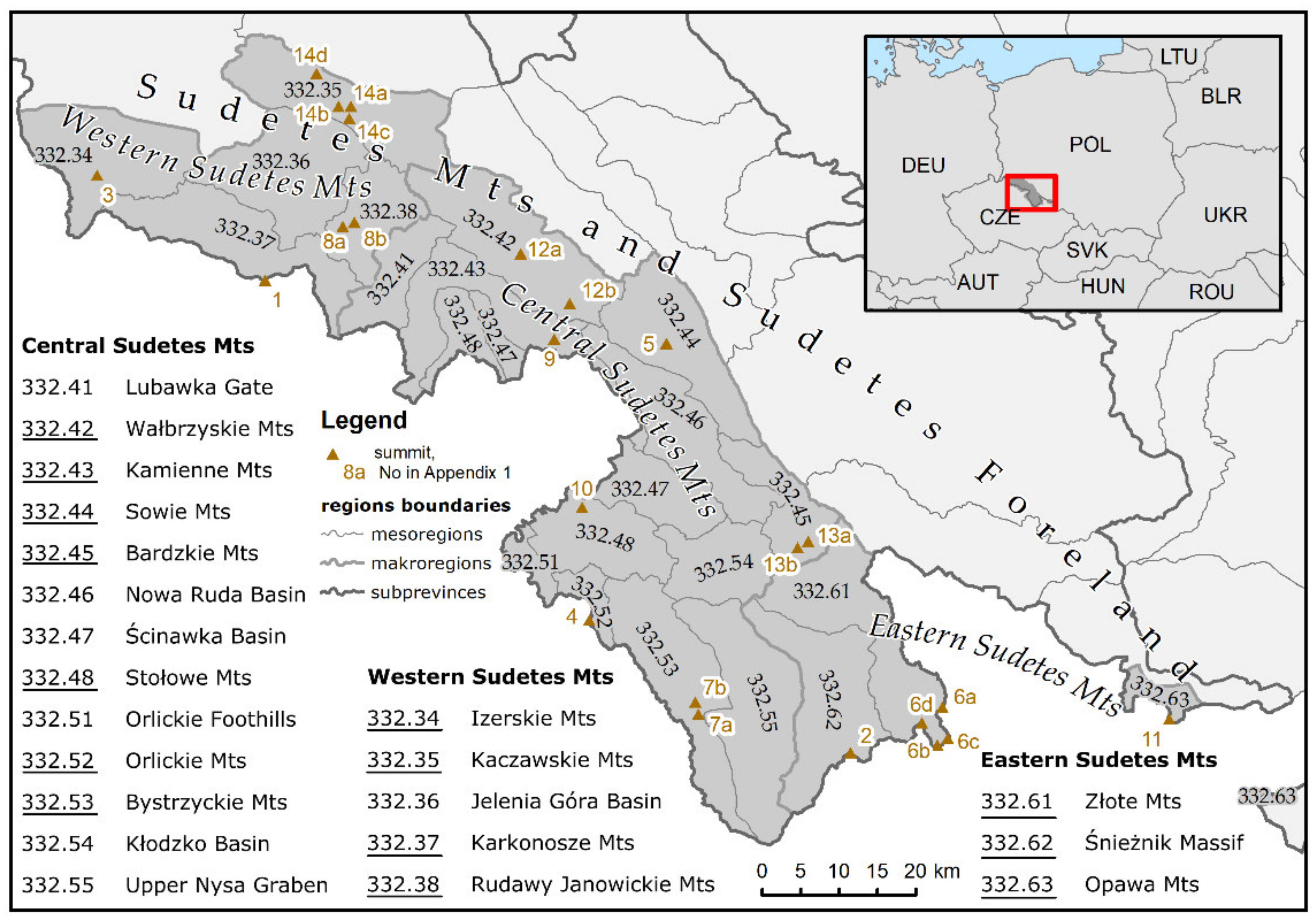
3. Sudetes Regionalisation

According to the current regionalisation of Poland, the country is divided into 344 mesoregions. These regions are determined based on geomorphological, geological and tectonic structures which are characteristic of a certain area and have an impact on its functioning. The current concept was developed by Solon et al. in 2018 [58] in response to legal regulations concerning landscape audits which required one to work at a scale of 1:50,000. The previous physico-geographical regionalisation of Poland, proposed by Kondracki [59], which was commonly used and accepted, was not accurate enough for scales larger than 1:500,000 [58].
The study area (mountain summits, Figure 2 & Table A1) was located in the Czech Massif province, the Sudetes Mountains and the Sudetes Foreland subprovince. The Czech Massif is a tectonic block composed of metamorphic and igneous rocks, Palaeozoic formations, and is partially covered by Cretaceous sandstone. In this area, fault-block mountains of 700 to 1600 m above sea level have formed [60].
The mountain ranges for which the highest summits were measured were chosen based primarily on the division into physico-geographical mesoregions [58]. Additional aspects considered were the customary names of the Sudetes mountain ranges. In general, mesoregions are not perceived as distinguishing features of mountain ranges. Some mountain ranges are traditionally designated for tourism; however, they tend to be too small to be considered a separate mesoregion. One example is the Bialskie Mountains located within the Złote Mountains mesoregion (in the Czech language: Rychlebské hory). The Złote Mountains are in the Eastern Sudetes and have a western border with the mesoregion of the Śnieżnik Massif (Table A1). The division of the region into geomorphological units adopted in the Czech Republic [61] (contrary to the historical Polish division [62]), does not distinguish the Bialskie Mountains as a separate geomorphological unit. In terms of physico-geographical units, Potocki [63] describes the region as ‘the Złote and the Bialskie Mts—Rychlebské hory’. The division into regions described by Potocki covers the entirety of the Sudetes, not just the Polish section. The Bialskie Mountains, as a separate range, are distinguished primarily through tourism. Under the Crown of Polish Mountains badge, which was initiated in 1997, the Bialskie Mountains and the Złote Mountains were distinguished separately [64]. In the division into mountain ranges applicable for the Diadem of the Polish Mountains badge [65], the authors found the mesoregions of the Bialskie Mountains and the Złote Mountains, and two microregions for these units. Due to their altitude, the Bialskie Mountains are often included in the Śnieżnik Massif region. This was the case for the PTTK Central Mountain Tourism Centre [66] and the authors of some maps and tourist guides [67,68]. Nowadays, most authors combine the Bialskie and the Złote Mountains into one mesoregion [69]. This approach was employed in this case.
Due to the previously described reservations regarding the separation of the Bialskie Mountains into a separate range, it was decided to measure the potential highest summits of the entire Złote Mountains mesoregion (and, thus, the Bialskie Mountains) and Mount Kowadło, which has the highest summit of the Złote Mountains excluding the Bialskie Mountains (Figure 3).
The mountains to be measured were selected based on an analysis of bibliographic and cartographic materials. As described in the Results section, more than a dozen sources measuring the height of the Sudetes Mountains (including ancient maps, scientific books, tourist publications, modern databases and datasets obtained using remote techniques) were analysed. Many historical sources replicate erroneous information about the highest peaks of the mountain ranges and/or their actual heights. For several mesoregions, the height of the peaks was clear (Złote Mountains) and for some mountains, there were several peaks in the literature depending on the source (the Golden Mountains). For other mesoregions, the mountains to be measured were chosen based on an analysis of LiDAR data (Kaczawskie Mountains). Ultimately, 24 mountains were selected for the 14 mesoregions that were analysed.

4. Materials and Methods

4.1. Altitude Determination Methods

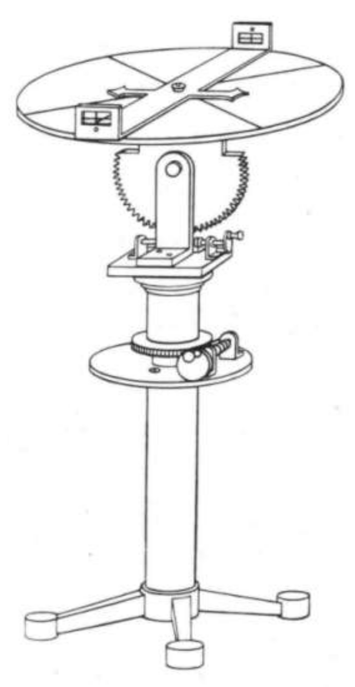
4.1.1. Historical Methods for Altitude Determination

The historical methods used to measure the altitude of mountains can be divided into three groups: geodetic methods, barometric methods and the boiling point method [70]. Geodetically, the altitude was determined by measuring triangles, levelling and measuring the distance from which the mountain was visible at sea. The first measurements of the altitude of mountains were taken in ancient Greece and Rome [71]. Altitude measurements were obtained using a simple instrument known as a dioptra (Figure 4). The altitude was calculated by analysing the mathematical relationship between the triangles.
The dioptra is a measurement tool that has been used for many centuries. Compared to modern methods, the levelling methods that have been used since ancient times are less inaccurate than methods that are based on the measurement of angles and lengths (in triangles). In the 16th and 17th centuries, the accuracy of surveying instruments improved and the theodolite (first constructed in 1576 by Joshua Habemel) replaced quadrants, astrolabes and dioptras [73]. The measurements also began to include, inter alia, atmospheric refraction. The measurement manuals that were created at that time describe, in detail, altitude and levelling measurements [74]. A milestone in geodetic measurement was the use of large-scale triangulation by Cassini [75]. The research conducted by the Cassini family in France (1666 to 1792) led to research in other countries, and the need to measure the altitude of mountains was increasingly articulated by the authors of measuring textbooks. An example was an instruction by Jan Śniadecki in 1790, which stated that the altitudes of mountains were necessary for the preparation of the national map [76]. The popularisation of barometers resulted in researchers using them to measure the altitude of mountains. Naturalists who did not commonly perform geometric measurements used barometers for altitude measurement due to their uncomplicated design. For example, in the 19th century, Karl Kolbenheyer used a barometer to take measurements in the Beskids [77]. Barometric measurements were also used by Adolf Traugott von Gersdorf in 1772 to calculate the summits of the Karkonosze Mountains; he set the altitude of Mount Śnieżka at 1598.4 m (The measurement was originally taken in toise (820.1 T); 1 T = 1.949 m) [78]. The least common method of measuring altitude involved measuring the decrease in the boiling point of water with increasing altitude. This method became popular in the 18th century. They were often used in conjunction with other methods, for example, in a study conducted by Humbolt during a trip to the Amazon [79]. Geometric methods and triangulation networks were used to determine the altitude of terrain points (including the altitude of mountains) using plain table measurements. For example, they were used during the second Austrian military topographic survey from 1806 to 1866 [80]. The average error in the altitude of the Tatra Mountain summits on this map was approximately 24 m. Until the introduction of satellite altitude measurement, the primary measurement method used in mountainous areas was (precise) trigonometric levelling [81]. These methods are also used nowadays as a complement to other methods. Taking into account numerous corrections made it possible to include trigonometric levelling in altitude measurements when establishing a geodynamic traverse in the Tatra Mountains [82].

4.1.2. GNSS

Currently, the GNSS is the most used geodetic measurement method for determining the position of a point, including the altitude. This method uses the known distance between the receiver’s antenna and the satellite. Based on this, the coordinates of the GNSS receiver are calculated. By using the autonomous GNSS measurement mode (measurements taken with a single receiver, without additional external data), position accuracy at one metre can be obtained, which in many cases is unsatisfactory. To increase the accuracy of position determination, differential measurements are used with the necessary fulfilment of two conditions—the use of phase data and the integer phase ambiguities. With the use of data made synchronously at the determined point, and at points with known coordinates (reference stations), observation errors are largely eliminated in the computational process. The differential processing of the measurement data provides accuracy within one centimetre.
Differential measurements are most often performed in static, RTK or network RTK (NRTK) mode (Figure 5). In static mode, a GNSS receiver is set at the point determined for a specified time. To obtain an altitude with an accuracy of several centimetres, the measurement should be performed for at least one hour. The greater the distance to the reference station, the longer the measurement time.
Conversely, the RTK/NRTK measurement is fast; a result is obtained immediately in the field but requires additional data to be sent from reference stations via the internet or radio. The RTK/NRTK technique allows for the altitude to be determined with an accuracy of approximately three to five centimetres [83] using a system of reference stations with a mean distance of 70 km between them.

4.1.3. LiDAR

LiDAR data provide information on the altitude of objects with finite accuracy. This accuracy is generally guaranteed for flat surfaces (e.g., bitumen roads, roofs) (Table 1). However, the quality of products delivered using large-area studies (with general goals) will be different than in the case of small areas developed for specific purposes. The algorithms used to classify the point cloud may be sensitive, primarily to terrain, vegetation, small landforms or buildings. In the ISOK project, general-purpose algorithms were used to classify point clouds and, therefore, local altitudes on the DTM or DSM models and the point cloud itself may have contained inaccuracies. These inaccuracies contributed to the difference in altitude between the GNSS measurements and the measurements obtained using LiDAR data.

4.1.4. Other Methods

Other methods used for altitude determination are classical ground surveying methods such as geometric or trigonometric levelling. However, nowadays, due to variable conditions in mountainous regions, these methods are generally used as supplementation for other techniques, for example, GNSS in locations with limited sky visibility [1,84]. Photogrammetry and remote sensing methods also play an important role in altitude determination. For example, terrestrial laser scanning may be used in combination with photogrammetric techniques for creating accurate DEMs from which the elevation values and surrounding terrain characteristics can be derived. This technology is useful, especially in steep regions or areas with various forms of terrain [85,86]. Photogrammetric techniques used for altitude determination are often based on aerial photographs taken from a plane or via unmanned aerial systems (UAS). The structure-from-motion (SfM) algorithm facilitates the creation of accurate and dense point clouds based on photographs that may then be used to create DTMs. The use of this approach, in combination with terrestrial laser scanning (TLS), has been reported by a team of Slovak researchers [86]. According to Sammartano and Spanò [87], DEMs derived from unmanned aerial vehicles (UAVs) can provide highly detailed morphological data of a similar quality to LiDAR and the implementation of this technique in the mapping of critical areas has shown promise. Overlapping aerial photographs or high-resolution satellite images can be processed more traditionally as stereo pairs. Studies have shown that it is possible to retrieve a 3D terrain structure based on information from the images and known camera or sensor parameters [88,89,90]. The interferometric synthetic aperture radar (InSAR) technique is another method that uses satellite images for altitude measurement [91,92].

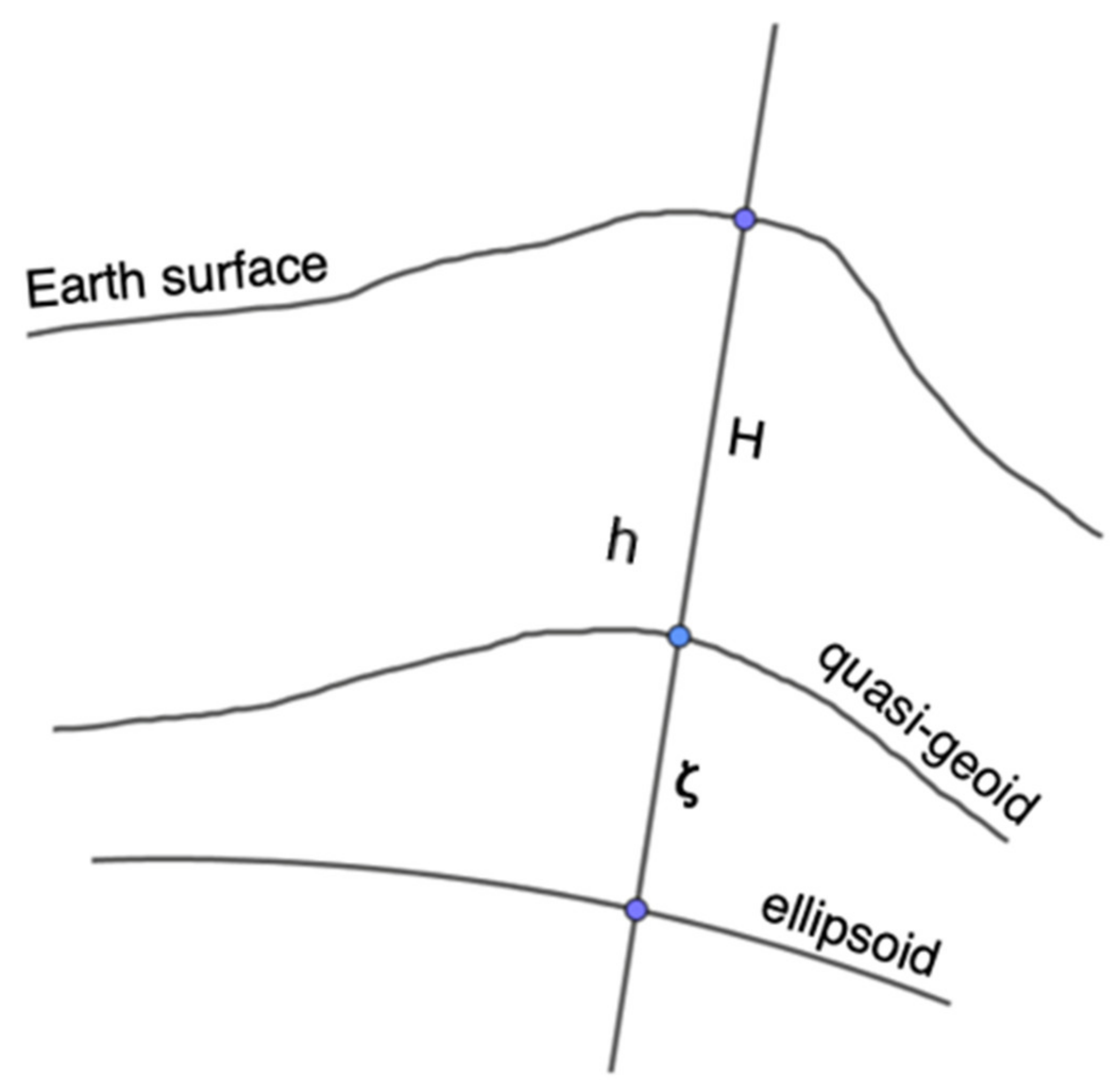
4.2. The Reference System and Geoid Models

The altitudes of mountain summits are given in relation to the adopted reference level, i.e., sea level (geoid or quasi-geoid surface). When using GNSS systems to determine altitude, the calculated height refers to the reference ellipsoid (Figure 6) and not to the sea level (geoid or quasi-geoid).
The distance of the ellipsoid from the geoid or quasi-geoid on Earth reaches 100 m, and this value must be included in the calculations. The geoid models that are currently available are at an accuracy of within one centimetre; however, their accuracy is generally lower in mountainous regions. In this case, the Polish model of the national quasi-geoid, PL-geoid-2011 [93] was used to calculate the normal height of the mountain summits.
Analyses of existing sources showed that the analysed area in the interwar period (the oldest sources analysed in this text) employed the orthometric height system referred to the mareograph in Amsterdam. In 1979, Poland switched to the normal height system referred to the Kronstad sea level, which has remained until today [94]. The differences between sea level in Amsterdam and Kronstad is +14 cm (Kronstad is higher, Figure 1). Calculated by the authors, the differences between the orthometric and normal height for the Snieżka Mountain (the highest peak in this article) leads to the 43.349 m geoid height (https://www.unavco.org/software/geodetic-utilities/geoid-height-calculator/geoid-height-calculator.html, accessed on 11 October 2020) and 43.690 m of quasi-geoid anomaly (http://www.gugik.gov.pl/bip/prawo/modele-danych, accessed on 11 October 2020). The maximum difference in this set of peaks is 34 cm (geoid is over quasi-geoid). Combining the orthometric heights referred to Amsterdam and normal height referred to the Kronstad led to a +48-cm difference for sources from the years 1918 to 1979. However, the bigger problem is the method of measurement and its accuracy, which is unknown.

4.3. Adopted Methodology

The measurement and verification of peak heights, assuming that the process was repeatable, required the research team to design the whole process accordingly. For organisational reasons, the workflow was divided into three sections (GIS, field and computing). According to the schema presented in Figure 7, the following work stages were planned:
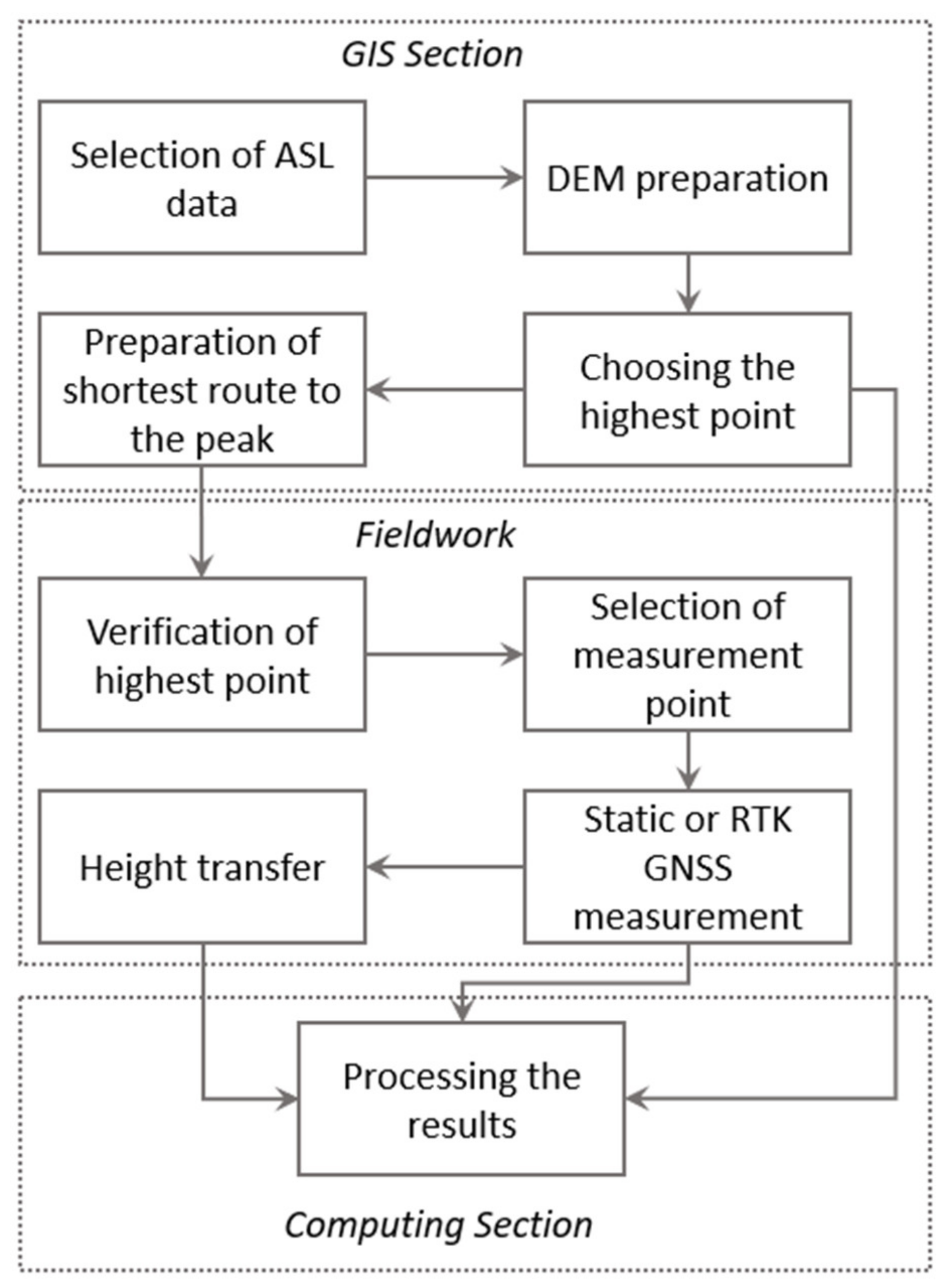
  • Selection of ASL data: the activity consisted in the selection of the specific fragment of ASL point cloud for the corresponding peak; here, the selection method was applied with a 3D buffer of 500 m radius;
  • The selected point cloud was the input data for DTM calculation; the natural neighbour method was used for grid interpolation from irregularly distributed points;
  • Finding the position of the highest point and optical verification of its position on the basis of available materials: orthophoto maps, satellite images, topographic maps and others. Since for some peaks the indication was ambiguous (small differences of one to five centimetres), it was decided to record data for more than one point;
  • Designing the measurement session by planning the access route, the stopping point and the route to the summit. At this point, measurement forms containing, among others, XYZ coordinates, a fragment of the base map, and a form to be completed during measurements were also created in an automated way;
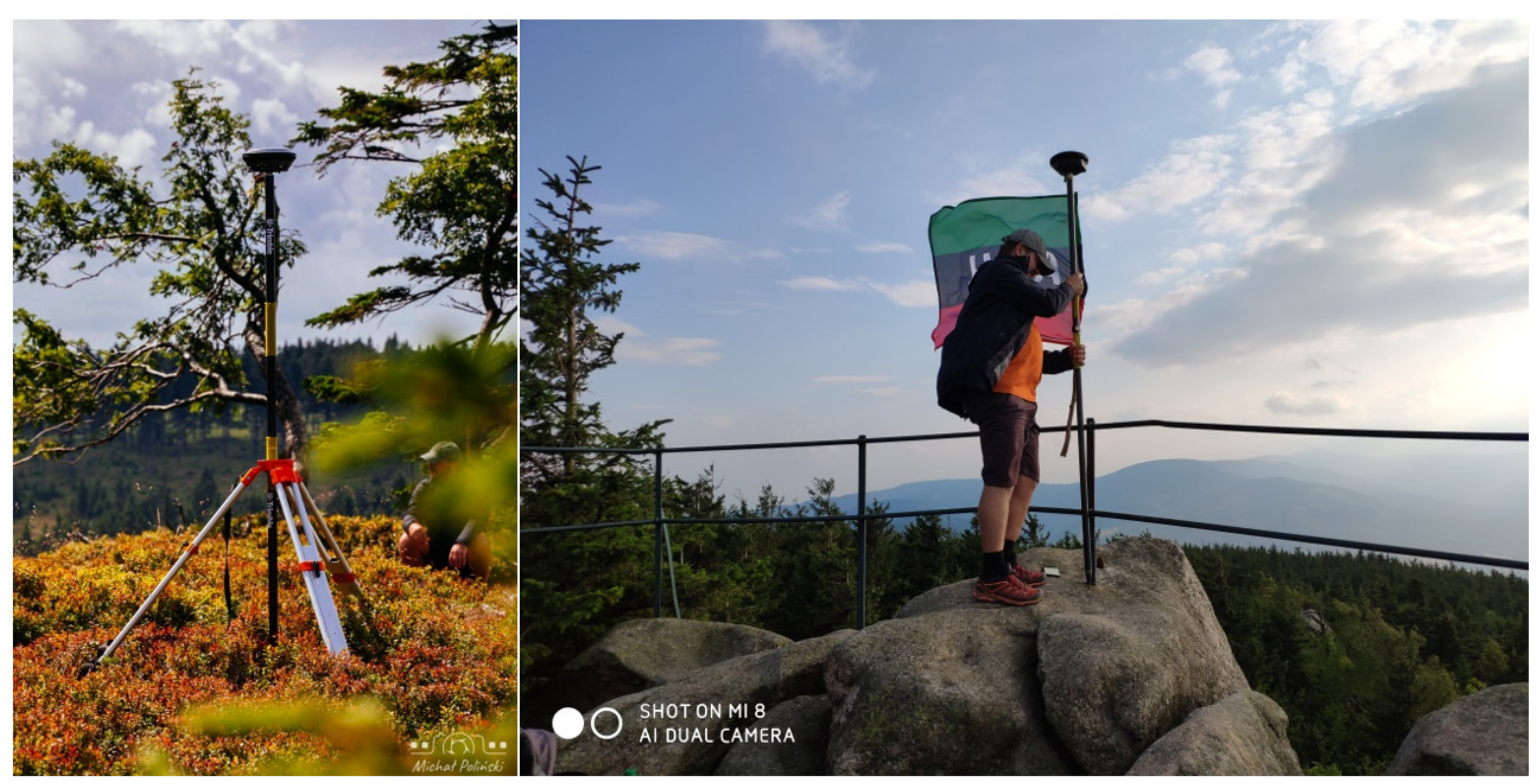
  • Upon reaching the summit, the height was verified using a GPS receiver (if possible) or a leveller. This allowed the selection of the highest point;
  • At this point, it was decided on the basis of local vision about the location of the measuring point; most often, it was a direct measurement on the point, and in four cases, an eccentric point was measured (Table 2);
  • GNSS measurement depending on possibilities using the RTK method or static method;
  • In the case of eccentric measurement, the height was transferred from the GNSS point to the highest point;
  • The last stage was calculating and recording of all data, intermediate results, measurements, and photo documentation in the database.
According to Table 1, the accuracy of the LiDAR measurement is 15 cm; to calculate the accuracy of the altitude determination by LiDAR, we should also include the quasi-geoid determination error, which can be adopted as 10 cm [93] for mountains areas. According to the rule of propagation of uncertainty, the final accuracy of the LiDAR measurements used in this paper is 18 cm. GNSS measurements taken with a Leica GS16 receiver were used to determine the altitudes. In the case of GSM signal availability and the possibility of a precise (fix) solution, the RTK network mode was used to obtain measurements using ASG-EUPOS reference stations and corrections. Each point was measured in this mode independently, three times, in 30-second sessions with a one-second interval. In each instance, after obtaining a precise solution, the receiver was disconnected, and initialisation was performed again to eliminate an incorrect initialisation error in the receiver. The final altitude was taken as the mean value of the three independent RTK measurement sessions.
When a precise RTK solution could not be obtained, one-hour static measurements with a one-second interval were taken. Static solutions were obtained in relation to two to five reference stations located less than 100 km from a measured point using LGO (Leica Geo Office 8.4) software. Precision IGS orbits were used for the solution.
For several of the measured points, it was impossible to use GNSS measurements due to significant obstacles on the horizon (mostly large trees). In this case, measurements were taken on an eccentric point (Table 2) with good GNSS satellite visibility. The height difference was transferred using a leveller and geometric levelling, with a maximum transfer error of ±0.5 cm.
The accuracy of the GNSS measurement was calculated according to the rule of propagation of uncertainty and consists of three components:
  • Quasi-geoid error—we assumed the maximum values from the model as 10 cm [93];
  • Positioning error—individual for each point at level 3 to 6 cm, based on the standard deviation from the post-processing software or RTK report (Table A1, column σG [m]);
  • Centring of the antenna and levelling error—0.02 cm;
The values for each summit are presented in column mG [m] in Table A1; based on the three errors mentioned above, the accuracy of determining the summit altitude by GNSS measurements does not exceed 12 cm.
At selected summits, GNSS measurements were obtained using a Xiaomi Mi8 smartphone equipped with a Broadcom BCM47755 chipset. This receiver allows for measurements to be taken on two frequencies: L1 and L5 for GPS and E1 and E5a for Galileo. The observations were recorded in sessions of one hour length, with a one-second recording interval. The measurement data were stored in the smartphone’s memory using the Geo++ receiver independent exchange (RINEX) Logger program in the RINEX format. The observations were post-processed using RTKLib software [95]. Due to the low quality of phase observations (a result of the large noise and cycle slips due to imperfect observation conditions) and very short measurement time (one hour), it was impossible to achieve integer or even float ambiguities; thus, only code pseudorange measurements were considered. Calculations were performed in single point positioning (SPP) mode. In case of the longer sessions, the accuracy might be improved by a larger number of observations; studies by other authors show much more accurate results, however, which included longer measurement sessions, e.g., [96,97].
The calculated ellipsoidal heights were transformed into the Kronstadt’86 national height reference system using the height anomaly from the PL-geoid-2011 quasi-geoid model [93]. The PL-geoid-2011 is the operational height system in the Polish territory.
LiDAR data processing at first required downloading appropriate datasets from www.geoportal.gov.pl (Polish national Geoportal run by the Head Office of Geodesy and Cartography, accessed on 14 October 2020). These were LiDAR point clouds and DTM data of 1 m × 1 m grid in ASCII format. Next, the data were imported to ArcGIS Pro 2.3.0 software, where all spatial analyses were conducted. This software, developed by the Esri Company, is a tool with various functions for analysing, visualising, image processing and map creation, both in 2D and 3D. At the initial stage, raster DTMs (which are interpolated based on LiDAR data) were loaded to the software and classified according to the pixel values representing heights. This made it possible to discover the highest points representing presumptive mountain peaks. Contour lines with labels were also generated to improve the usability and visualisation of the data. Next, LiDAR point clouds were loaded to the software and the highest LiDAR measurements classified as ‘ground’, were found in the vicinity of the highest DTM pixel values. These height values are described in the Results section. The highest LiDAR points were treated as the basis for the fieldwork with GNSS. Their coordinates were calculated in PL-1992 (EPSG: 2180) and PL-2000 (EPSG: 2176, 2177) projections to simplify the process of searching for them in the mountains.
Examining the historical sources of altitude data requires source criticism methods which is the interdisciplinary study of how information sources are evaluated for given tasks. This method was employed in this study. Data used by the authors of other studies were also analysed and used as a reference for altitude information evaluation. Overall, in relation to a given purpose (e.g., altitude data), a particular information source may be valid, reliable or relevant. The most common, reliable sources, such as scientific books, guidebooks and maps, were chosen for this study. Furthermore, altitude data in old maps were analysed. The least issue is the problem with the reference system and mareograph (sea level). First of all, in the Austria-Hungary context, there was an orthometric height system with mareograph in Trieste, before WWI. Between the interwar period, there was an orthometric height system referred to as the Amsterdam mareograph. The differences between the Kronstad tide-gauges for Trieste and Amsterdam were 48 and −14 cm, respectively [57]. After WWII, the Kronstad mareograph and normal heights became a reference for the polish height system. The authors calculated the maximum difference between the normal and orthometric height systems for Śnieżka peak (the highest of the analysed summits, 1603 m).

5. Results

The results of this study are summarised in Appendix A Table A1. The altitude data received from professional GNSS devices often differed from the data used in maps, guidebooks and scientific books. It was also observed that many tourist maps and guidebook publishers used altitude data that was established using outdated technology. Furthermore, in general, the data received from those sources were remarkably similar. A detailed analysis is presented below.
Column 1 in Table A1 displays the heights taken from articles about each mountain on Polish-language Wikipedia pages. The authors do not treat data from Wikipedia as a source of measurement data. Instead, the purpose of including Wikipedia as a data source was to demonstrate the most popular information used by the public and to critically analyze it. In Wikipedia, the height of a mountain peak can be written in several places (in the infobox, in the text of the article or on the mountain range page). The values were obtained on November 6, 2020. The height of a mountain was recorded from the most accurate value given in Wikipedia. In a situation where the article contained several values for the height of a mountain, the most recent measurement was used, or the measurement was confirmed by a reliable source in the bibliography. For one peak (Mount Okole), the value in parentheses was obtained from an article about the Kaczawskie Mountains and this value was used in the study. It should be noted that, on Wikipedia, there are no community-accepted rules concerning the specification of altitude for features such as mountains. Most often, heights are provided with one metre accuracy, although there are also situations in which heights are provided with decimetre or centimetre accuracy. The differences in the values between columns 1 and 7 for most peaks (n = 17), was less than one metre. For an additional four peaks, the difference was not greater than two metres (Mount Postawna, −1.3 m; Mount Szeroka Góra, 1.3 m; Mount Wysoka Kopa, 1.6 m and Mount Folwarczna, 1.8 m) and three peaks differed in height by more than two metres (Mount Skopiec, 2.1 m; Mount Szczeliniec Wielki, 2.7 m and Mount Ostra Mała, 9.8 m). The data on peak heights presented in Wikipedia are unreliable, despite relatively small differences observed compared with the GNSS measurements (Table A1, Appendix A, Columns (G)NSS and (L)iDAR contains data from Supplementary Materials project). Credible data sources are only provided for individual mountains. The large difference in altitude recorded for Mount Ostra Mała was because historical height measurements did not account for the rock formation at its peak. It was also observed that only the heights of 9 out of 24 peaks were provided in the WikiData project, which is intended to be the source for the data presented in Wikipedia.
Column 2 (Table A1) [98] contains heights obtained from the official website of the Crown of Polish Mountains (CPM) tourist badge [64] and column 7 displays the heights of the geomorphological regions [62]. The altitude values of the mountains obtained in this study will be presented as a sample bibliographic source for the authors of the CPM badge. The differences in column 7 were only noted for the Bialskie Mountains, for which the authors probably gave the height of Mount Travná Hora, the peak of which is already on the Czech side (1025 m). Furthmore, this column does not include a height for the Opawskie Mountains because the maximum height was not provided in the source publication. When the differences between the GNSS measurements and the values in columns 2 and 7 were compared, the majority of the height values provided in the sources contained large errors. The largest differences were recorded for Mount Chełmiec (the Wałbrzyskie Mountains), −19.0 m; Mount Kłodzka Góra (the Bardzkie Mountains), −7.8 m and Mount Skopiec (the Kaczawskie Mountains), −3.3 m. In column 2, a large difference in values was also observed for Mount Rudawiec (−5.8 m). A comparison of the results of this study with data presented on the official website of the CPM tourist badge showed that several summits included in the summary were not the highest peaks in the listed regions (according to our measurements). It should be noted that each of the large differences in values was negative, which indicates that the heights of those mountains included objects located at the peak (e.g., an 18 m high lookout tower is present at the summit of Mount Chełmiec) or that errors occurred during reproduction from old cartographic materials. The similarity of values also suggests that the creators of the CPM tourist badge may have used geomorphological regionalisation as a source of height data. It was not clear where the height values on the CPM tourist badge website originated from. The original summary of the mountains was established in 1997, based on the sources available at that time [64] and should not be treated as referential.
Column 3 (Table A1) contains height values obtained from the labels on the interactive map at mapa-turystyczna [99]. The heights on this site are provided with one metre accuracy. For 16 of the peaks, the difference between the GNSS measurements and the values in column 2 did not exceed +/− 1 m. For five of the peaks, the height differences measured up to +/− 2 m, and for four of the peaks, they exceeded this value (Mount Śnieżnik, −3 m; Mount Ostra Mała, 8.8 m; Mount Szczeliniec Wielki, 2.7 m; Mount Okole, 3.3 m). Of all the differences in values, only six were below 0. The heights obtained from the mapa-turystyczna.pl (accessed on 1 October 2020) website originated from digitised analogue maps. According to the website administrators, the point heights were derived from the shuttle radar topography mission (SRTM). The aim of this mission was to collect digital elevation data of the Earth’s surface with a 1-arc-second resolution (approximately 30 m). The analysed map showed differences between the heights recorded in the database (used, for example, by the search engine) and those obtained from the labels on the map. The label values were derived from the OpenStreetMap database or digitised analogue maps. The large differences observed between the GNSS measurements and the heights recorded on the mapa-turystyczna.pl website occurred because rock formations located on the mountain tops or the height of the state triangulation obelisk (on Mount Śnieżnik) were not accounted for on the maps.
The above-mentioned data originated from Internet sources whereas the data in columns 6 to 12 (Table A1) were derived from printed sources (primarily guidebooks and scientific books). In these columns, most of the altitude data presented are similar to each other (±1 m). However, in several cases, the difference in values was up to 16 m (the highest peak of Mount Postawna in the Złote Mountains) compared to data from Chanaś et al. (1974) and Sarosiek et al. (1975) [100,101] (Table A1, columns 8 and 9). A difference was also observed for the highest peak of the Wałbrzyskie Mountains (Mount Chełmiec), where when the data from Sarosiek, et al. (1975) and AGP (2020) were compared, the difference was 35 metres [101,102]. Moreover, according to our GNSS measurements (column 13), Mount Chełmiec was not the highest mountain—Mount Borowa was. Furthermore, Chanaś, et al. (1974) suggested that Mount Borowa was the highest peak of the Wałbrzyskie Mountains [100].
The GNSS measurements were also compared with the heights provided by the Head Office of Geodesy and Cartography (GUGiK) in the form of a web service [103]. This service (NMT service) facilitates height determination for any point located in Poland. The XY coordinates were obtained from the National Register of Geographic Names (PRNG) [104]. PRNG is a public database (provided by GUGiK) that stores the location and attributes of geographic objects in Poland. This database stores information about mountain peaks and their location. Nowadays, due to the NMT service being made available by GUGiK, information on peak heights has been removed from the PRNG database. There are 23 of 24 measured peaks in the PRNG, and the heights obtained from the NMT service are provided in column 5 (Table A1). For three of the peaks (Mount Rudawiec, Mount Kowadło and Mount Postawna), the height difference between the values in columns 4 and 12 was less than 0. For the remaining 20 peaks, the differences in height values were greater than 0. For three other peaks, the height differences ranged from just under 10 m to greater than 10 m (Mount Okole, 9.9 m; Mount Ostra Mała, 10.6 m; Mount Szczeliniec Wielki, 11.4 m). The height differences for five of the peaks measured between one and five metres, and for the remaining 12 peaks the height difference did not exceed one metre. These results confirmed that, in most cases, the summit coordinates stored in the PRNG did not represent the highest point. The height differences of a few metres and a dozen or so metres were observed for peaks with large rock formations. The height differences less than zero may have resulted from the misclassification of the LiDAR point cloud for peaks covered with vegetation. In summary, a combination of two sources—the PRNG database and the NMT service, provided by the GUGiK—did not provide reliable information on the height of the peaks.
The altitudes determined based on LiDAR data were compared with the altitudes acquired from GNSS measurements. The results are presented in Appendix A Table A1. The differences in altitude derived from GNSS and LiDAR measurements are presented in column ‘G-L [m]’ and the values ranged from −4.2 m to 2.4 m. Assuming the GNSS technique provided a higher accuracy compared to LiDAR, it should be emphasised that in five cases, the altitudes were the same for both methods (Mount Śnieżka, 1603.2 m; Mount Waligóra, 934.3 m; Mount Biskupia Kopa, 889.8 m; Mount Chełmiec, 850.0 m and Mount Borowa, 853.4 m). Besides Mount Waligóra (934.3 m), whose summit is covered with trees, the other summits can be characterised by existing buildings and good sky visibility. Mount Szczeliniec Wielki (921.7 m, for which the difference between GNSS and LiDAR measurements was as small as 0.1 m) is located in an open area, and with its rocky summit, the landforms are easily differentiated. For eight of the summits, the difference in values indicated that LiDAR-derived points were located higher than those measured via GNSS (negative difference values). The largest difference in values (−4.2 m) was observed for Mount Śnieżnik (1423.0 m). In this case, the LiDAR elevation value referred to the altitude of the watchtower remains and not to the ground. This confirmed the assumption that the automatic classification of ground points may produce accidental errors in the output classification. Mount Skopiec (720.7 m) and Mount Kowadło (988.0 m) were the second and third summits with the largest negative difference in altitude values (−2.2 and −1.7 m, respectively). In these cases, the inconsistencies may have been the result of an incorrect LiDAR point classification to the ‘ground’ class. The top of Mount Skopiec is covered with vegetation that might have been the cause of errors. Mount Kowadło has a barren mountain summit and the error most likely occurred as a result of the laser beam being reflected off people or other objects located at the top of the mountain when the LiDAR measurements were obtained. Values with a negative difference for other summits ranged from −0.3 to −0.7 m (−0.3 m for Mount Brusek (1115.5 m), −0.4 m for Mount Postawna (977.2 m), −0.6 m for Mount Jagodna Północna (984.5 m), −0.7 m for Mount Rudawiec (1106.2 m) and −0.7 m for Mount Jagodna (977.2 m). Each of these mountains has different characteristics. The summit of Mount Brusek is not covered with vegetation and Mount Postawna is peatland-like, with sparse spruce stands and bilberries. At the summit of Mount Jagodna Północna, there is a young spruce forest, and the neighbouring Mount Jagodna and Mount Rudawiec have barren summits. In the case of values with a positive difference, the GNSS measurements were higher than the LiDAR measurements. For eight of the summits, this difference did not exceed 0.5 m (0.2 m for Mount Orlica (1084.5 m) and Mount Kłodzka Góra (757.2 m); 0.3 m for Mount Wysoka Kopa (1127.6 m), Mount Skalnik (944.5 m), Mount Szeroka Góra (766.3 m) and Mount Baraniec (720.1 m); and 0.4 m for Mount Wielka Sowa (1015.7 m) and Mount Ostra Mała (944.8 m)). The characteristics of each of these summits are different; several are covered with trees, and others are barren, composed of rocks or including buildings. Overall, the observed differences were the result of LiDAR data processing procedures.
Two of the peaks, Mount Folwarczna (Maślak) (724.7 m) and Mount Okole (725.3 m), showed larger differences. These values were 1.8 m and 2.4 m, respectively. Mount Folwarczna has a grassy summit and Mount Okole has a rocky peak with significantly elevated landform features (Figure 8). There are many potential reasons for the large difference observed between the GNSS and LiDAR values. However, the analysis of the data suggests that it resulted from accidental errors produced during the LiDAR point cloud classification.
Smartphone GNSS measurements were obtained on four summits of the Sudetes: Mount Śnieżnik, Mount Szczeliniec Wielki, Mount Orlica and Mount Borowa. The altitudes of the mountain summits (HS), standard deviations σHs and the deviations from height values determined by the RTK (or static) method (dHG-S) are shown in Table 3.
Difficult measurement conditions (primarily obstruction of the horizon) resulted in slightly larger deviations for Mount Szczeliniec Wielki and Mount Borowa. In the case of smartphone measurements, the accuracy of the altitude determination of the peaks obtained in this study is considered typical for the SPP method that was applied.

6. Discussion

6.1. A Comparison of the Methods for Altitude Determination: Pros and Cons

The results of this study highlighted the differences between the GNSS and LiDAR methods, suggesting the advantage of a direct method over an indirect method. When assuming an accuracy of one metre for elevation data, the results of the LiDAR technique corroborated the GNSS measurements in many cases. If one accuracy was assumed, the results demonstrate that differences equal to or greater than one metre were observed for 8 of the 24 mountains examined. Moreover, neither the source of these differences nor the characteristic features that may have caused them could be determined. Therefore, the primary conclusion is that the LiDAR method should be used with criticism for altitude determination. It should be noted, however, that this conclusion applies to LiDAR datasets with such parameters as those described in this study. It is the opinion of the authors that the use of LiDAR datasets for altitude determination should be supported by cartographic and photogrammetric analysis.
The primary advantage of GNSS measurements is that they are usually easy to obtain, and the measurement takes place at a well-identified point. However, to obtain the most accurate altitude measurements, attention should be paid to the planning of a site with an open horizon. In the present study, the accuracy for determining the normal height (above sea level) was estimated at approximately eight centimetres, taking into account the GNSS technique measurement errors (a maximum error of five centimetres was assumed [83]) and the error for the quasi-geoid model (PL-geoid-2011) used in the Sudetes area (a maximum error of six centimetres was assumed [93]).
The accuracy of measurements obtained via the Xiaomi Mi8 smartphone were much lower than that offered by professional geodetic-class GNSS receivers (Table 3). This confirmed the results obtained by other authors [13,14]. However, the smartphone data cannot provide equivalent performance to that provided by geodetic-grade receivers (with one of the main reasons being the difference in the quality of the antenna used in smartphones) [18,96,97]. The rapid development of algorithms and measuring techniques adapted to the specifics of mobile devices can be expected in the near future. This will most likely be due to the widespread availability of smartphones and great interest from scientific and research centres, as well as potential users of such solutions [105]. Access to code and phase observations offers new perspectives for the use of mobile devices in precise positioning. Due to the portability of smartphones, their use in mountainous conditions would be particularly beneficial. However, at present, the quality of smartphone GNSS phase measurements is insufficient to obtain high accuracy in altitude determination.

6.2. Can a Modification of the Altitude of (the Highest) Summits Influence Tourism in Those Regions?

The quest for the highest summit of a mountain range has fascinated researchers in the past and remains captivating nowadays [84]. Apart from the imperative of describing ‘reality’, which instructs researchers to take more accurate measurements, this action has an impact on other areas (e.g., tourism). The highest altitude is provided as a description of an area in many classifications (physico-geographical, geomorphological, natural). Due to its interdisciplinary foundations, the most common division is physico-geographical mesoregions. Besides its scientific value, this division is also recommended to be used for land description by local government [106]. Due to the difficulties involved in taking direct measurements on mountain summits, it is important to employ surveyors to aid in the verification process. Similar to the present study, research on the measurement of the highest mountain summits is conducted globally [107].
In the Sudetes, the most important impact on tourism visitation is a modification of the highest summits in individual mountain ranges. This is because many climbers ascend to the highest summit, considering it to be the most prestigious, making this a valuable achievement. Additionally, many people are bagging for summits belonging to the highest points of the Polish Mountains. This list includes 28 summits in the Polish part of the Sudetes, the Carpathians and the Holy Cross Mountains (or the Świętokrzyskie Mountains). Within the Sudetes, 14 summits are included on the list of the highest points of the Polish Mountains. According to the GNSS research conducted in this study, as many as five mountains in the Sudetes should lose their titles as the highest summits in the range:
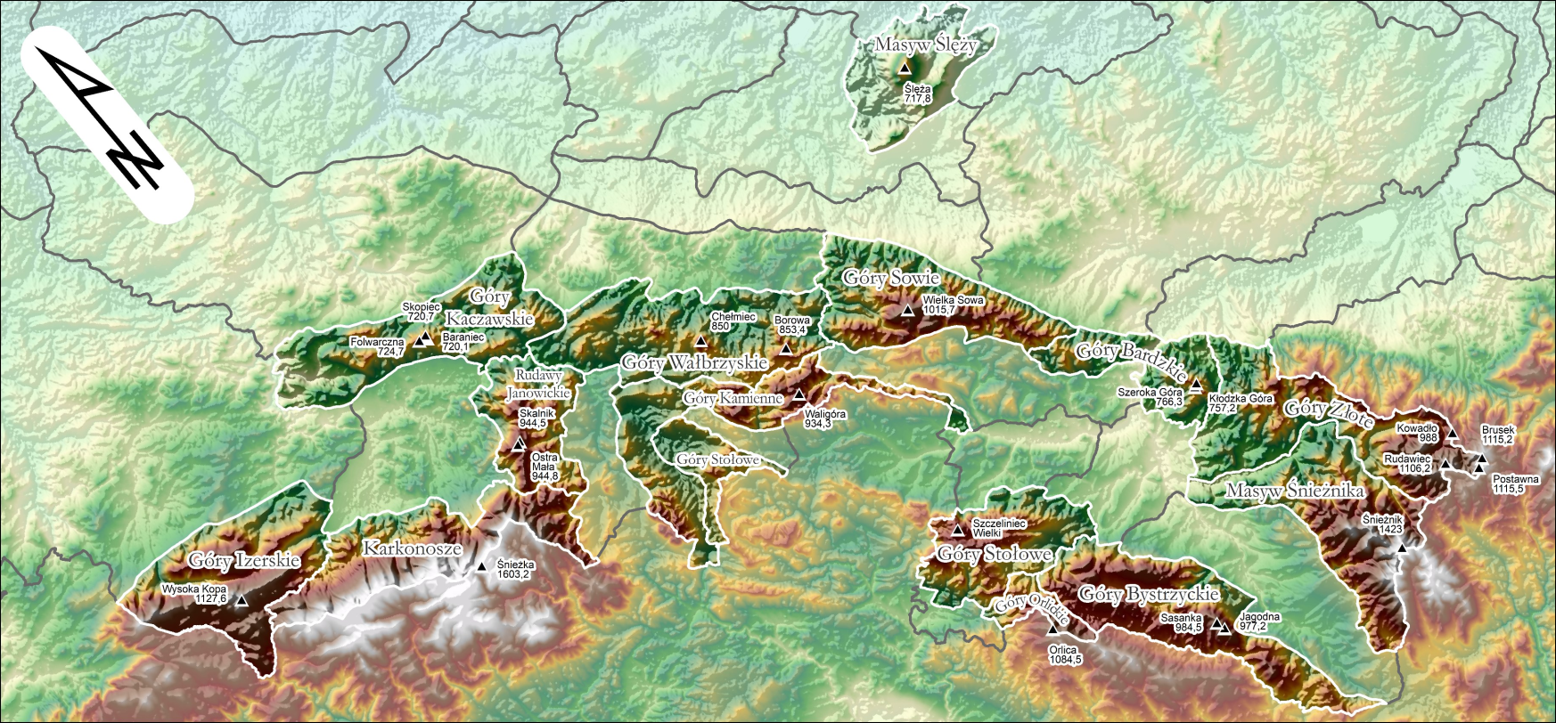
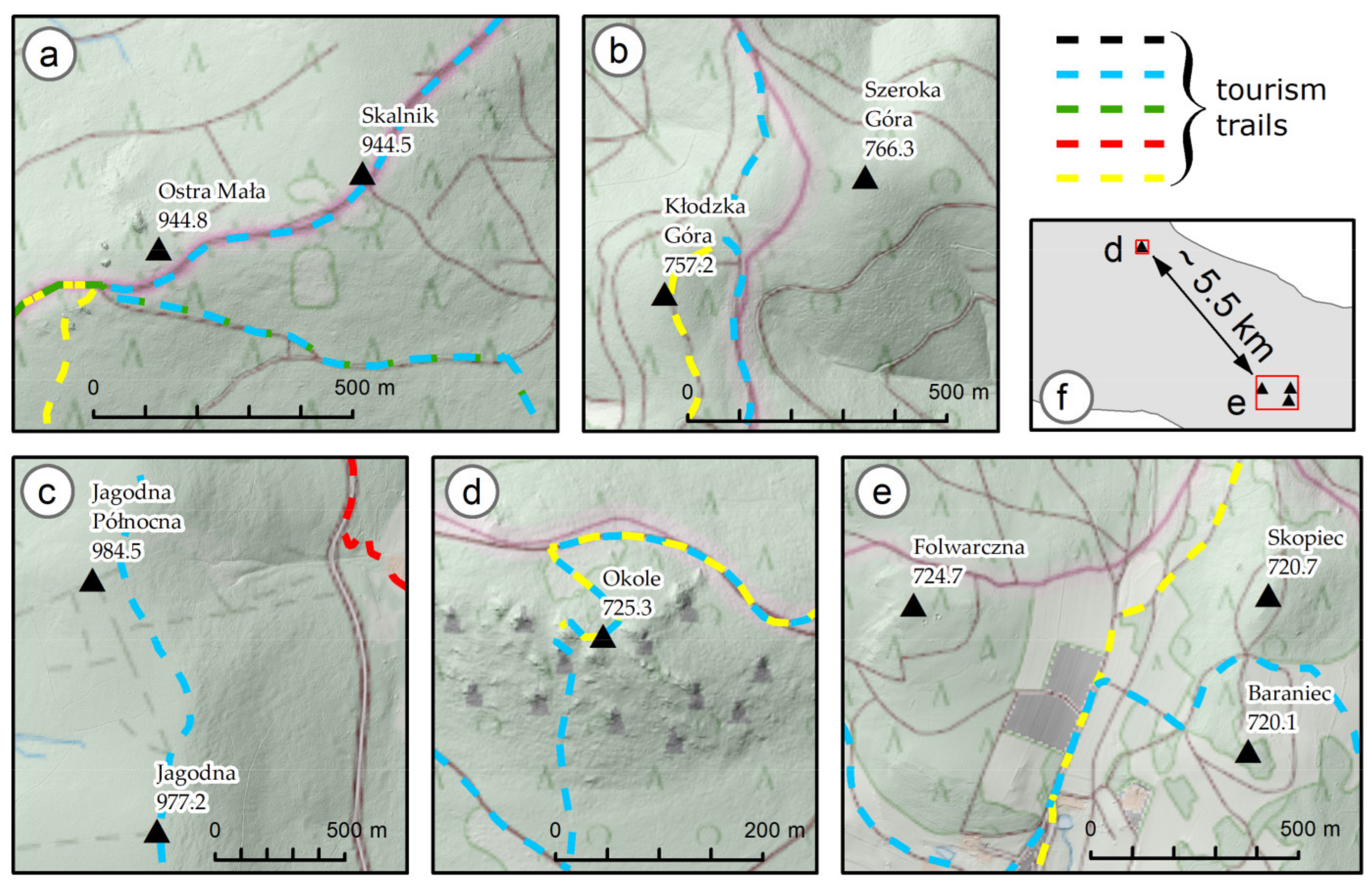
  • The Rudawy Janowickie Mountain Range (Figure 9a): Mount Skalnik (944.5 m) lost its title to Mount Ostra Mała (944.8 m). In this case, the differences were extremely small, which may cause further controversy. Mount Ostra Mała is situated a short distance off the trail (approximately 150 m from the crossing of the yellow, green, blue and red trails (the main Sudetes trails)). It should be noted that Mount Ostra Mała is part of Mount Skalnik;
  • The Bardzkie Mountain Range (Figure 9b): Mount Kłodzka Góra (757.2 m) to Mount Szeroka Góra (766.3 m). Mount Szeroka Góra is off the trail (approximately 300 m from the blue trail). Moreover, Mount Szeroka Góra (the highest in the range, according to our calculations) lies within the same mountain as the top of Mount Kłodzka Góra (previously considered the highest);
  • The Bystrzyckie Mountain Range (Figure 9c): Mount Jagodna (977.2 m) lost its title to Mount Jagodna Północna (984.5 m). Mount Jagodna Północna is off the trail (approximately 100 m from the blue trail);
  • The Kaczawskie Mountain Range (Figure 9d–f): Mount Skopiec (720.7 m) to the summit of Mount Okole (725.3 m). Mount Okole is off the trail (approximately 30 m from the blue trail). As many as four summits were considered for the title of the highest summit of the Kaczawskie Mountains (in addition to the previously mentioned summits, Mount Folwarczna and Mount Baraniec were also included). Moreover, Mount Okole is a lesser known summit;
  • The Wałbrzyskie Mountain Range: Mount Chełmiec (850 m) to Mount Borowa (853.3 m). Mount Borowa is on the trail (red and black). Moreover, in the Wałbrzyskie Mountains, Mount Borowa has long been recognised by tourists as the highest mountain in the range. Many tourists climb this summit and Mount Chełmiec.
Therefore, due to the large modifications that must be made to mountain altitudes, the present form of the highest points of Polish the Mountains should be questioned. In general, peak-baggers still continue to climb the wrong peaks and the situation is similar in the Carpathians and the Świętokrzyskie Mountains. Furthermore, there is a new geographical division into regions. The inaccuracy of the current list has been raised for years. This has lead to an initiative known as ‘The Great Crown of Polish Mountains’ covering 40 summits and including all the mountains that are considered doubtful as the highest [108]. An alternative initiative is The Diadem of the Polish Mountains [65].
Since this study focused only on the Polish section of the mountains, the conditions in the Czech portion of the mountain range remain unclear. The territory on the Czech side is an important area of spatial concentration for winter and summer recreation centres [109]. According to a study conducted by Stursa [110], the Karkonosze Mountains are among the most visited national parks in Europe. The difference between the highest summit and the ‘second-highest’ summit is relatively large for most of the mountains on the Czech side. However, we discovered three geomorphological units in which a possible change of several metres could mean a revision of the list i.e., The Jizera Mountains (Mount Smrk, 1124 m and Mount Jizera, 1122 m) (mesoregion 332.34, Figure 1), the Rychlebské Mountains (Mount Srmk, 1127 m and Mount Travná hora, 1124 m) and the Broumov Highlands (Mount Královecký Špičák, 881 m and Mount Ruprechtický Špičák, 880 m) (mesoregion 332.43, Figure 1). However, potential changes to the tourist infrastructure are not necessary as the highest summits of the Jizera Mountains and the Broumov Highlands are accessible along a marked tourist trail. Unlike Mount Smrk, Mount Travná hora is outside the marked trails of the Rychlebské Mountains. However, tourist attendance for Mount Smrk is considerably limited, as the summit is part of a small-scale protection area. A study from the border mountains of the Šumava demonstrated that locals appreciate the value of natural locales and want to protect those areas [111].
Due to the maximum altitude of the Czech mountains (max. 1602 m), the 1000 m limit is important in terms of tourist attractiveness. Certain tourist products and projects encourage the attainment of a summit exceeding 1000 m [112,113], of which there are 395 in the Czech Republic. Several of the summits, which are many metres below 1000 m, are also located in the Czech part of the Sudetes Mountains, for example, Mount Suchý vrch (995 m, in the Orlické Mountains) or Mount Studniční vrch (992 m, in the Rychlebské Mountains). Tourist competitions promote the achievement of predefined summits to make an area appear more attractive; this is the case with cycling in the Czech Republic. In the monitored region of the Czech border, four relevant competitions take place, including the Mountaineering Crown of Cyclists (Mountaineering Crown of Jeseníky, Sudetenland, Eastern Bohemia and the North) [114]. Many of them localise points in Poland. However, the defined points are not only summits but are also other attractive places in the territory. The organisers of the competitions strive to show the diversity of the territory and they deliberately avoid certain tourist-exposed areas; the site selection is also based on bicycle accessibility.
It should be noted that when routes are changed, the flows of tourism traffic may also change (a different area of interest, a commuting change, parking facilities, accommodation, catering services, etc.). Additionally, certain well-known trails such as the Main Beskid Trail [115] should also be modified to run through the highest and, therefore, more attractive summits. From a marketing point of view, if the product is set as a journey connecting the highest summits, it is necessary to redefine the path or the core of the product. More often than not, people who partake in mountain activities focus not only on the attractiveness of a mountainous region but also the ease of access [3]. Thus, determining the missing routes is the most urgent task for the managers of the Sudetes. However, it is necessary to respect the limits arising from the protection of the territory [110]. Many of the monitored summits are part of large-scale protected areas, which restrict the arbitrary creation and marking of new roads and the construction of accompanying tourist infrastructure. An additional issue is the need for modification of the altitude values on maps and guides, among other sources.
Although, as numerous studies have shown, LiDAR data must be used with caution, especially when the altitude of the summits are to be altered. The results of this study also demonstrate this via the comparisons presented in Table A1. Without an understanding of this, information chaos can occur, resulting in users distrusting maps and guides, and tourists doubting geographic and geodetic research and information.

7. Conclusions

The main problems we encountered while analysing the problem described in this paper and the conclusions related to it were:
  • By investigating an entire mountain range, this research demonstrated the need for verification of the altitude of peaks and verification of which peak is the highest. For the Sudetes Mountains, in most printed sources, old altitude data were later reproduced in other (more recent) editions of the Sudetes guidebooks or changed to new, ‘inaccurate’ ones. A comparison of these altitude data with our GNSS measurements demonstrated the need for an update of the Internet and book sources. Furthermore, LiDAR should be used as a first-stage method (before professional GNSS field measurements), as its accuracy is questionable. This study highlights the urgent need for the correction of peak heights. In general, people trust maps and books and expect the information they contain to be accurate. Moreover, altitude data are usually relied upon by authors in various research activities. Thus, the primary conclusion of this study is not only the need for altitude corrections but also the need for improvement of the accuracy of data on the Internet and in printed sources. Furthermore, as mentioned earlier, Wikipedia is freely accessible by the public (e.g., using this research as a source); however, in the case of books and maps, only publishers and authors can cease reproduction of old and inaccurate data. After this article is published, the authors will disseminate information about mountain heights and the highest peaks in each mesoregion by including the study data in the WikiData database. Therefore, the data will be easily accessible in all languages. The altitude information (and the location of the highest point of a mountain) must be included in official topographic maps. This can only happen if the contractors of these maps are obliged to use correct data sources such as PRNG. In this database, height information can be recorded as comments. An alternative method could be to manually edit the DTM rasters and give one cell representing the highest point of the mountain the correct height. Perhaps the GUGiK would decide to take such a step in the next tender for large-scale LiDAR data acquisition. For this reason, it is crucial to record significant mountain heights in a public database such as the PRNG. Information on mountain heights, based on GNSS measurements, LiDAR data analysis and a literature query, would be reliable for the producers of topographic maps. Technical standards for topographic map preparation indicate the numerical terrain model as the source for elevation points. This is one of the few exceptions because most objects on Polish contemporary topographic maps were created using the Database of Topographic Object (BDOT10k) as a source. The names of the mountains originate directly from the PRNG database. The standards do not specify where the value for the height of a mountain should come from. Therefore, it is necessary to disseminate knowledge about the importance of using supplementary GNSS measurements for mountain peak altitudes, as demonstrated in this study. The sources compared in the article were suggested for use by the geodetic administration in Poland. It was a NMT service, which allows users to obtain heights for any point from the territory of Poland. The connection of this website with a database storing information about geographical objects (National Register of Geographic Names) allowed the authors to treat it as the official source of altitude data. This service is based on data from airborne laser scanning. The same data (but used in a different way) was compared in the article. This allowed for a critical analysis of this data source, which, when used incorrectly (but recommended by the administration), provides erroneous results. The authors found no such comparison in the literature;
  • The approach used in the article allows for the minimization of errors in the future by using this type of data in determining the height of mountains. These analyses seem important not only for Polish researchers but also for a constantly growing number of other countries in Europe and worldwide, where LiDAR datasets are becoming more freely accessible to anyone interested;
  • Moreover, measurements from the LiDAR in this text were made by creating hydrological maps; thus, it cannot be treated as a reliable source for mountain altitude determination. The ‘theoretica’ error calculated by the authors is 18 cm, while comparison with GNSS results lead up to a couple of metres;
  • Altitude obtained from direct GNSS measurements are the most accurate and reliable from all techniques currently used. In the worst-case error, this can lead to a 12 cm difference;
  • The most important issue is the differences between GNSS and LiDAR. If the altitudes from LiDAR are bigger than from GNSS, the source of the error might be caused by the incorrect classification (e.g., grass or trees in top). In our case, the majority of the altitudes from LiDAR are smaller than GNSS and bigger than the accuracy (18 cm) factor, which cannot be treated as the classification issue, more like ‘real’ LiDAR accuracy;
  • The last but most important issue is a global problem of the data sources. Most of the available data on the Internet are based on the DTM from the LiDAR data; our paper shows that these altitudes cannot be treated as reliable and differences between ‘true’ values can be up to a few metres.

8. Limitations

Not all mountain summits are readily accessible for altitude measurement. During the planning of fieldwork, the potential highest points were determined; however, only the on-site verification revealed difficulties. The following barriers to measuring altitude were identified:
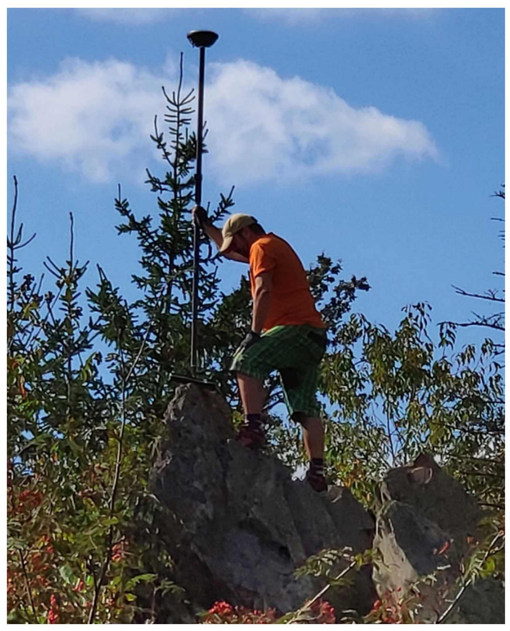
  • Steep inselbergs making it difficult to stabilise the measuring instrument (Figure 8);
  • High vegetation at the summit site making it difficult to take GNSS measurements (Figure 10a);
  • Low vegetation making it difficult to identify the highest point of the summit (Figure 10a);
  • Technical infrastructure not related to tourism (Figure 10b);
  • Tourist infrastructure (e.g., on Mount Borowa);
  • Rocks at the summit that were not permanently attached to the ground (e.g., loose mounds of stones on Mount Wysoka Kopa).
Each of the above-mentioned issues was solved thanks to the presence of a measurement team on each of the summits. The method used most frequently was to obtain a levelling measurement and transfer the altitude to a point available for GNSS measurement. In cases where it was difficult to identify the highest point at the summit, it was also searched for with the use of a leveller via a series of measurements taken at several points.

Supplementary Materials

The following data are available online at http://koronagor.agh.edu.pl/.

Author Contributions

Conceptualisation, K.M., M.A., J.M.C., O.K., K.K., J.K., J.M., M.R., B.S., S.S.; methodology, K.M., M.A., J.M.C., O.K., K.K., J.K., J.M., M.R., B.S., S.S.; software, K.M., M.A., J.M.C., O.K., K.K., J.K., J.M., M.R., B.S., S.S.; validation, K.M., M.A., J.M.C., O.K., K.K., J.K., J.M., M.R., B.S., S.S.; formal analysis, K.M., M.A., J.M.C., O.K., K.K., J.K., J.M., M.R., B.S., S.S.; investigation, K.M., M.A., J.M.C., O.K., K.K., J.K., J.M., M.R., B.S., S.S.; resources, K.M., M.A., J.M.C., O.K., K.K., J.K., J.M., M.R., B.S., S.S.; data curation, K.M., M.A., J.M.C., O.K., K.K., J.K., J.M., M.R., B.S., S.S.; writing—original draft preparation, K.M., M.A., J.M.C., O.K., K.K., J.K., J.M., M.R., B.S., S.S.; writing—review and editing, K.M., M.A., J.M.C., O.K., K.K., J.K., J.M., M.R., B.S., S.S.; visualisation, K.M., M.A., J.M.C., O.K., K.K., J.K., J.M., M.R., B.S., S.S.; supervision, K.M., M.A., J.M.C., O.K., K.K., J.K., J.M., M.R., B.S., S.S.; project administration, K.M., M.A., J.M.C., O.K., K.K., J.K., J.M., M.R., B.S., S.S.; funding acquisition, K.M., M.A., J.M.C., O.K., K.K., J.K., J.M., M.R., B.S., S.S. Author Contributions: K.M. 20%, M.A. 10%, J.M.C. 5%, O.K. 5%, K.K. 10%, J.K. 10%, J.M. 10%, M.R. 10%, B.S. 10%, S.S. 10%. All authors have read and agreed to the published version of the manuscript.

Funding

This research was funded by the ‘Setka w Koronie. Korona Gór Polski na 100-lecie AGH’ project (http://koronagor.agh.edu.pl/).

Institutional Review Board Statement

Not applicable.

Informed Consent Statement

Not applicable.

Data Availability Statement

Not applicable.

Acknowledgments

This research was funded by subvention number 16.16.150.545.

Conflicts of Interest

The authors declare no conflict of interest.

Appendix A

Table A1. The altitude above sea level of the highest summits in the Sudetes Mountains according to maps, guidebooks, summit signs, and LiDAR and GNSS measurements.
NoSummit (24)Mountain Range (14)Heights Sources [m]G-L [m]
Internet SourcesPaper SourcesCalculated
(1)(2)(3)(4)(5)(6)(7)(8)(9)(10)(11)(12)(G)NSSσG [m]mG [m](L)iDAR
1ŚnieżkaKarkonosze Mts1603.31602.01603.01603.31603.01603.01602.01602.01605.01603.01602.01602.01603.20.030.111603.20.0
2ŚnieżnikŚnieżnika Massif1423.01425.01426.01425.01422.91425.01425.01425.01422.01426.01425.01425.01423.00.050.111427.2−4.2
3Wysoka KopaIzerskie Mts1126.01126.01126.01126.01127.01126.01126.01126.01127.01126.01126.01126.01127.60.060.121127.30.3
4OrlicaOrlickie Mts1084.01084.01084.01079.81080.4 1084.01084.01080.01084.01084.01084.01084.50.050.111084.30.2
5Wielka SowaSowie Mts1015.01015.01015.01014.01015.31014.01015.01015.01015.01015.01015.01015.01015.70.030.111015.30.4
6aKowadłoZłote Mts988.0989.0988.0987.6988.3 990.0987.0 989.0988.0988.00.030.11989.7−1.7
6bPostawna1116.81112.01117.0-1115.7 1125.01125.01109.0 1115.50.050.111115.9−0.4
6cBrusek1115.91116.0-1114.7 1124.0 1115.20.060.121115.5−0.3
6dRudawiec1106.41106.01106.21106.9 1106.20.040.111106.9−0.7
7aJagodnaBystrzyckie Mts977.2977.0977.0977.2976.9978.0978.0977.0977.0977.0977.0977.0977.20.040.11977.9−0.7
7bJagodna Północna985.0985.0978.0- 984.50.040.11985.1−0.6
8aSkalnikRudawy Janowickie Mts944.0945.0944.0940.0943.7935.0945.0945.0945.0945.0945.0945.0944.50.030.11944.20.3
8bOstra Mala935.0936.0945.0934.2 944.80.050.11944.40.4
9WaligóraKamienne Mts933.9936.0934.0936.0933.9 936.0936.0936.0936.0936.0936.0934.30.060.12934.30.0
10Szczeliniec WielkiStołowe Mts919.0919.0919.0919.1910.3919.0919.0919.0919.0919.0919.0919.0921.70.060.12921.60.1
11Biskupia KopaOpawskie Mts890.0889.0891.0890.3886.1 -889.0889.0 890.0891.0889.80.050.11889.80.0
12aChełmiecWałbrzyskie Mts851.0869.0851.0-849.8850.0869.0-834.0 851.0869.0850.00.030.11850.00.0
12bBorowa853.3853.0853.1853.2 854.0853.0853.0853.0853.0853.40.030.11853.40.0
13aKłodzka GóraBardzkie Mts757.0765.0757.0762.0756.4762.0765.0765.0762.0765.0765.0765.0757.20.030.11757.00.2
13bSzeroka Góra765.0766.0-765.5 740.0 766.30.060.12766.00.3
14aSkopiecKaczawskie Mts718.6724.0719.0724.1718.2 724.0724.0724.0720.0724.0724.0720.70.030.11720.40.3
14bFolwarczna722.9723.0-722.2 720.0- 724.70.050.11722.91.8
14cBaraniec720.3720.0723.3718.7 -723.0720.0720.10.050.11719.80.3
14dOkole718 (725.1)722.0721.0715.4 721.0721.0714.0 725.30.040.11722.92.4
(1) Wikipedia–Articles about individual peaks on the Polish Wikipedia website—A detailed description can be found in Section 5, paragraph 2 (data downloaded on November 6, 2020). (2) Korona Gór Polski [64,98]. (3) Mapa-turystyczna [99]. (4) Archiwum Map Wojskowego Instytutu Geograficznego 1919–1939 [116]. (5) National Register of Geographic Names [104] and NMT service [103]. (6) Koszarski (1963) W Sudetach [117]. (7) Walczak (1972) Sudety i Pogorze Sudeckie [118]. (8) Chanaś (1974) Sudety. Przewodnik [100]. (9) Sarosiek (1975) Sudety [101]. (10) Czerwiński (1996) Sudety. Przewodnik [119]. (11) Szewczyk (2013) Sudety dla aktywnych [120]. (12) Collective work (2020) Atlas Gór Polski. Szczyty w zasięgu ręki [102].

References

  1. Kozioł, K.; Maciuk, K. New heights of the highest peaks of Polish mountain ranges. Remote Sens. 2020, 12, 1446. [Google Scholar] [CrossRef]
  2. Apollo, M.; Mostowska, J.; Maciuk, K.; Wengel, Y.; Jones, T.E.; Cheer, J.M. Peak-bagging and cartographic misrepresentations: A call to correction. Curr. Issues Tour. 2020, 1–6. [Google Scholar] [CrossRef]
  3. Apollo, M. The true accessibility of mountaineering: The case of the High Himalaya. J. Outdoor Recreat. Tour. 2017, 17, 29–43. [Google Scholar] [CrossRef]
  4. Zurick, D.N. Adventure Travel and Sustainable Tourism in the Peripheral Economy of Nepal. Ann. Assoc. Am. Geogr. 1992, 82, 608–628. [Google Scholar] [CrossRef]
  5. Nyaupane, G.P. Mountaineering on Mt Everest: Evolution, economy, ecology and ethics. In Mountaineering Tour; Taylor and Francis Inc.: Oxfordshire, UK, 2015; pp. 265–271. ISBN 9781317668732. [Google Scholar]
  6. Apollo, M. Dual Pricing—Two Points of View (Citizen and Non-citizen) Case of Entrance Fees in Tourist Facilities in Nepal. Procedia Soc. Behav. Sci. 2014, 120, 414–422. [Google Scholar] [CrossRef] [Green Version]
  7. Pérez, O.J.; Hoyer, M.; Hernández, J.; Rodríguez, C.; Márques, V.; Sué, N.; Velandia, J.; Fernandes, J.; Deiros, D. GPS height measurement of peak bolivar, venezuela. Surv. Rev. 2006, 38, 697–702. [Google Scholar] [CrossRef]
  8. Auh, S.C.; Lee, S.B. Analysis of the Effect of Tropospheric Delay on Orthometric Height Determination at High Mountain. KSCE J. Civ. Eng. 2018, 22, 4573–4579. [Google Scholar] [CrossRef]
  9. TeamKILI2008. Precise Determination of the Orthometric Height of Mt. Kilimanjaro. In Proceedings of the FIG Working Week, Eilat, Israel, 3–8 May 2009; p. 11. [Google Scholar]
  10. European Global Navigation Satellite Systems Agency (GSA). White Paper on Using GNSS Raw Measurements on Android Devices; Publications Office of the European Union: Luxembourg, 2017. [Google Scholar] [CrossRef]
  11. Realini, E.; Caldera, S.; Pertusini, L.; Sampietro, D. Precise GNSS Positioning Using Smart Devices. Sensors 2017, 17, 2434. [Google Scholar] [CrossRef] [PubMed] [Green Version]
  12. Lachapelle, G.; Gratton, P.; Horrelt, J.; Lemieux, E.; Broumandan, A. Evaluation of a Low Cost Hand Held Unit with GNSS Raw Data Capability and Comparison with an Android Smartphone. Sensors 2018, 18, 4185. [Google Scholar] [CrossRef] [Green Version]
  13. Robustelli, U.; Baiocchi, V.; Pugliano, G. Assessment of Dual Frequency GNSS Observations from a Xiaomi Mi 8 Android Smartphone and Positioning Performance Analysis. Electronics 2019, 8, 91. [Google Scholar] [CrossRef] [Green Version]
  14. Wielgocka, N.; Hadaś, T. Czy to już koniec? Geodeta 2019, 4, 8–12. [Google Scholar]
  15. Wu, Q.; Sun, M.; Zhou, C.; Zhang, P. Precise Point Positioning Using Dual-Frequency GNSS Observations on Smartphone. Sensors 2019, 19, 2189. [Google Scholar] [CrossRef] [PubMed] [Green Version]
  16. Uradziński, M.; Bakuła, M. Assessment of Static Positioning Accuracy Using Low-Cost Smartphone GPS Devices for Geodetic Survey Points’ Determination and Monitoring. Appl. Sci. 2020, 10, 5308. [Google Scholar] [CrossRef]
  17. Gogoi, N.; Minetto, A.; Linty, N.; Dovis, F. A Controlled-Environment Quality Assessment of Android GNSS Raw Measurements. Electronics 2018, 8, 5. [Google Scholar] [CrossRef] [Green Version]
  18. Paziewski, J.; Fortunato, M.; Mazzoni, A.; Odolinski, R. An analysis of multi-GNSS observations tracked by recent Android smartphones and smartphone-only relative positioning results. Measurement 2021, 175, 109162. [Google Scholar] [CrossRef]
  19. Fernandez Diaz, J.C.; Carter, W.E.; Shrestha, R.L.; Glennie, C.L. LiDAR Remote Sensing. In Handbook of Satellite Applications; Pelton, J., Madry, S., Camacho-Lara, S., Eds.; Springer New York: New York, NY, USA, 2020; pp. 1–52. [Google Scholar]
  20. National Oceanic and Atmospheric Administration (NOAA) Coastal Services Center. Lidar 101: An Introduction to Lidar Technology, Data and Applications; NOAA Coastal Services Center: Charleston, SC, USA, 2012.
  21. Wężyk, P. (Ed.) Informatyczny System Osłony Kraju Przez Nadzwyczajnymi Zagrożeniami. Podręcznik dla Uczestników Szkoleń z Wykorzystania Produktów LiDAR, 2nd ed.; Główny Urząd Geodezji i Kartografii: Warszawa, Poland, 2015; ISBN 9788325421007. [Google Scholar]
  22. Kurczyński, Z. Fotogrametria (Photogrammetry); PWN: Warszawa, Poland, 2014. [Google Scholar]
  23. White, R.A.; Dietterick, B.C.; Mastin, T.; Strohman, R. forest roads mapped using LiDAR in steep forested terrain. Remote Sens. 2010, 2, 1120–1141. [Google Scholar] [CrossRef] [Green Version]
  24. Wężyk, P.; Borowiec, N.; Szombara, S.; Wańczyk, R. Generation of Digital Surface and Terrain Models of the Tatras Mountains based on Airborne Laser Scanning (ALS) Point Cloud. Arch. Photogramm. Photogramm. Cartogr. Remote Sens. 2008, 18, 651–661. [Google Scholar]
  25. Migoń, P.; Kasprzak, M.; Traczyk, A. How high-resolution DEM based on airborne LiDAR helped to reinterpret landforms—examples from the Sudetes, SW Poland. Landf. Anal. 2013, 22, 89–101. [Google Scholar] [CrossRef]
  26. Helfricht, K.; Kuhn, M.; Keuschnig, M.; Heilig, A. Lidar snow cover studies on glaciers in the Ötztal Alps (Austria): Comparison with snow depths calculated from GPR measurements. Cryosphere 2014, 8, 41–57. [Google Scholar] [CrossRef] [Green Version]
  27. Farías-Barahona, D.; Ayala, Á.; Bravo, C.; Vivero, S.; Seehaus, T.; Vijay, S.; Schaefer, M.; Buglio, F.; Casassa, G.; Braun, M.H. 60 years of glacier elevation and mass changes in the Maipo River Basin, central Andes of Chile. Remote Sens. 2020, 12, 1658. [Google Scholar] [CrossRef]
  28. Hopkinson, C.; Demuth, M.; Sitar, M.; Chasmer, L. Applications of airborne LiDAR mapping in glacierised mountainous terrain. Int. Geosci. Remote Sens. Symp. 2001, 2, 949–951. [Google Scholar] [CrossRef]
  29. Chrustek, P.; Wężyk, P. Using High Resolution LiDAR Data to Estimate Potential Avalanche Release Areas on the Example of Polish Mountain Regions. In Proceedings of the ISSW 09—International Snow Science Workshop, Innsbruck, Austria, 7–12 October 2018; pp. 495–499. [Google Scholar]
  30. Luo, Y.; Ma, H.; Zhou, L. DEM Retrieval From Airborne LiDAR Point Clouds in Mountain Areas via Deep Neural Networks. IEEE Geosci. Remote. Sens. Lett. 2017, 14, 1770–1774. [Google Scholar] [CrossRef]
  31. Chrisman, N.R. The error component in spatial data. Geogr. Inf. Syst. 1991, 1, 165–174. [Google Scholar]
  32. Yan, L.; Lee, M.Y. Are tourists satisfied with the map at hand? Curr. Issues Tour. 2015, 18, 1048–1058. [Google Scholar] [CrossRef]
  33. Kudrys, J.; Buśko, M.; Kozioł, K.; Maciuk, K. Determination of the normal height of Chornohora summits by a precise modern measurement techniques. Maejo Int. J. Sci. Technol. 2020, 14, 156–165. [Google Scholar]
  34. Collier, P.A.; Croft, M.J. Heights from GPS in an engineering environment. Surv. Rev. 1997, 34, 76–85. [Google Scholar] [CrossRef]
  35. Featherstone, W.E.E.; Dentith, M.C.C.; Kirby, J.F.F. Strategies for the accurate determination of orthometric heights from GPS. Surv. Rev. 1998, 34, 278–296. [Google Scholar] [CrossRef]
  36. Poretti, G.G. Reporter 47—The Magazine of Leica Geosystems; Leica Geosystems AG: Heerbrugg, Switzerland, 1999; pp. 28–29. [Google Scholar]
  37. Ward, M. The height of Mount Everest. Alp. J. 1995, 100, 30–33. [Google Scholar] [CrossRef]
  38. Wright, K. Measuring Mount Everest. Discover 2000, 36, 38. [Google Scholar]
  39. Chen, J.; Zhang, Y.; Yuan, J.; Guo, C.; Zhang, P. Height Determination of Qomolangma Feng (MT. Everest) in 2005. Surv. Rev. 2010, 42, 122–131. [Google Scholar] [CrossRef]
  40. Saburi, J.; Angelakis, N.; Jaeger, R.; Illner, M.; Jackson, P.; Pugh, K.T. Height measurement of Kilimanjaro. Surv. Rev. 2000, 35, 552–562. [Google Scholar] [CrossRef]
  41. Ulotu, P. Mount Kilimanjaro Orthometric Height by TZG08 Geoid Model and GPS Ellipsoidal Heights from 1999 and 2008 GPS Campaigns. J. Land Adm. East Afr. 2020, 2. Available online: https://www.researchgate.net/profile/Prosper-Ulotu-3/publication/315831204_Mount_Kilimanjaro_Orthometric_Height_by_TZG08_Geoid_Model_and_GPS_Ellipsoidal_Heights_from_1999_and_2008_GPS_Campaigns_Journal_of_Land_Administration_East_Africa/links/5e27f59e92851c3aadcfb742/Mount-Kilimanjaro-Orthometric-Height-by-TZG08-Geoid-Model-and-GPS-Ellipsoidal-Heights-from-1999-and-2008-GPS-Campaigns-Journal-of-Land-Administration-East-Africa.pdf (accessed on 14 February 2021).
  42. Muller, J.-C. The Concept of Error in Cartography. Cartogr. Int. J. Geogr. Inf. Geovisualization 1987, 24, 1–15. [Google Scholar] [CrossRef] [Green Version]
  43. Cater, E.; Mieczkowski, Z. Environmental Issues of Tourism and Recreation. Geogr. J. 1996, 162, 338. [Google Scholar] [CrossRef]
  44. Beedie, P.; Hudson, S. Emergence of mountain-based adventure tourism. Ann. Tour. Res. 2003, 30, 625–643. [Google Scholar] [CrossRef]
  45. Ryan, C. Recreational Tourism: Demand and Impacts; Channel View Publications: Clevedon, UK, 2003; Volume 43, ISBN 0047287504272. [Google Scholar]
  46. Caber, M.; Albayrak, T. Push or pull? Identifying rock climbing tourists’ motivations. Tour. Manag. 2016, 55, 74–84. [Google Scholar] [CrossRef]
  47. Burke, S.M.; Durand-Bush, N.; Doell, K. Exploring feel and motivation with recreational and elite Mount Everest climbers: An ethnographic study. Int. J. Sport Exerc. Psychol. 2010, 8, 373–393. [Google Scholar] [CrossRef]
  48. Lew, A.A.; Han, G. A World Geography of Mountain Trekking. In Mountaineering Tour; Taylor and Francis Inc.: Oxfordshire, UK, 2015; pp. 19–39. ISBN 9781317668732. [Google Scholar]
  49. Kuby, M.J.; Wentz, E.A.; Vogt, B.J.; Virden, R. Experiences in developing a tourism web site for hiking Arizona’s highest summits and deepest canyons. Tour. Geogr. 2001, 3, 454–473. [Google Scholar] [CrossRef]
  50. Crockett, L.J.; Murray, N.P.; Kime, D.B. Self-Determination Strategy in Mountaineering: Collecting Colorado’s Highest Peaks. Leis. Sci. 2020, 1–20. [Google Scholar] [CrossRef]
  51. Leick, A.; Rapoport, L.; Tatarnikov, D. GPS Satellite Surveying, 4th ed.; John Wiley & Sons, Inc.: Hoboken, NJ, USA, 2015; ISBN 9781119018612. [Google Scholar]
  52. Kleusberg, A.; Teunissen, P.J.G. GPS for Geodesy; Otto, J.-C., Dikau, R., Eds.; Lecture Notes in Earth Sciences; Springer: Berlin/Heidelberg, Germany, 1996; Volume 115, ISBN 3-540-60785-4. [Google Scholar]
  53. Seeber, G. Satellite Geodesy; Walter de Gruyter: Berlin/Heidelberg, Germany; New York, NY, USA, 2003; ISBN 9783110200089. [Google Scholar]
  54. Hwang, C.; Hsiao, Y.-S.; Lu, C.; Wu, W.-S.; Tseng, Y.-H. Determination of Northeast Asia’s Highest Peak (Mt. Jade) by Direct Levelling. Surv. Rev. 2007, 39, 21–33. [Google Scholar] [CrossRef]
  55. Xiang, H.; Cao, C.; Jia, H.; Xu, M.; Myneni, R.B. The analysis on the accuracy of DEM Retrieval by the Ground Lidar Point Cloud Data Extraction Methods in Mountain Forest Areas. In Proceedings of the International Geoscience and Remote Sensing Symposium (IGARSS), Munich, Germany, 22–27 July 2012; pp. 6067–6070. [Google Scholar]
  56. Pawłuszek, K.; Borkowski, A.; Ziaja, M. Ocena dokładności wysokościowej danych lotniczego skaningu laserowego systemu ISOK na obszarze doliny rzeki Widawy. Acta Sci. Pol. Geod. Descr. Terrarum 2014, 13, 27–37. [Google Scholar]
  57. Kurałowicz, Z.; Słomska, A. Stacje Mareograficzne i Wybrane Wysokościowe Układy Odniesienia w Europie. Inżynieria Morska i Geotechnika 2015, 843–853. Available online: https://yadda.icm.edu.pl/baztech/element/bwmeta1.element.baztech-b49dec3b-348b-4d5e-abed-9ff1bc971dc5 (accessed on 14 February 2021).
  58. Solon, J.; Borzyszkowski, J.; Bidłasik, M.; Richling, A.; Badora, K.; Balon, J.; Brzezińska-Wójcik, T.; Chabudziński, Ł.; Dobrowolski, R.; Grzegorczyk, I.; et al. Physico-geographical mesoregions of Poland: Verification and adjustment of boundaries on the basis of contemporary spatial data. Geogr. Pol. 2018, 91, 143–170. [Google Scholar] [CrossRef]
  59. Kondracki, J.; Richling, A. Mapa 53.3. Regiony fizycznogeograficzne. In Atlas Rzeczypospolitej Polskiej; IGiPZ PAN, Główny Geodeta Kraju, PPWK im. E. Romera: Warszawa, Poland, 1994. [Google Scholar]
  60. Kondracki, J. Geografia Regionalna Polski, 2nd ed.; PWN: Warszawa, Poland, 2000; ISBN 9788301130503. [Google Scholar]
  61. Úřad, Z. Geomorfologické Jednotky ČR. Available online: https://geoportal.cuzk.cz/(S(lfbleuq3wxtolown0jzp4lib))/Default.aspx?mode=TextMeta&side=wms.AGS&metadataID=CZ-CUZK-AGS-GEOMORF&metadataXSL=metadata.sluzba&head_tab=sekce-03-gp&menu=3144 (accessed on 12 October 2020).
  62. Walczak, W. Sudety i Przedgórze Sudeckie. In Geomorfologia polski, Tom 1 Polska południowa, góry i wyżyny; Klimaszewski, M., Ed.; Państwowe Wydawnictwo Naukowe: Warszawa, Poland, 1972; pp. 173–174. [Google Scholar]
  63. Potocki, J. Funkcje Turystyki w Kształtowaniu Transgranicznego Regionu Górskiego Sudetów; Wrocławskie Towarzystwo Naukowe: Wrocław, Poland, 2009; ISBN 978-83-7374-061-7. [Google Scholar]
  64. Lewandowski, W.; Więckowski, M. Korona Gór Polski. Poznaj Swój Kraj 1997, XL, 17. [Google Scholar]
  65. PTTK Komisja Turystyki Górskiej Oddział Wrocławski Diadem Polskich Gór. Available online: http://www.ktg.wroclaw.pl/diadem.php (accessed on 15 October 2020).
  66. Zarząd_Główny_PTTK; Kmisja_Turystyki_Górskiej_PTTK; Komisja_Turystyki_Narciarskiej. Górska Odznaka Turystyczna PTTK, Odznaki narciarskie PTTK; Centralny Ośrodek Turystyki Górskiej PTTK: Kraków, Poland, 2015; ISBN 978-83-62473-59-5. [Google Scholar]
  67. Mazurski, K.R. Masyw Śnieżnika i Góry Bialskie; Oficyna Wydawnicza Oddziału Wrocławskiego PTTK: Wrocław, Poland, 1995; ISBN 83-8555048-8. [Google Scholar]
  68. Compass. Masyw Śnieżnika, Góry Bialskie; Gmina Stronie Śląskie: Stronie Śląskie, Poland, 2017; ISBN 9788376058283. [Google Scholar]
  69. Badora, K. Proposition for physico-geographical regionalization of Eastern Sudetes. Pract. i Stud. Geogr. 2018, 63, 59–73. [Google Scholar]
  70. Cajori, F. History of Determinations of the Heights of Mountains. ISIS 1929, 12, 482–514. [Google Scholar] [CrossRef]
  71. Lewis, M.J.T. Surveying Instruments of Greece and Rome; Cambridge University Press: Cambridge, UK, 2004; ISBN 0511031939. [Google Scholar]
  72. Heron. Heronis Alexandrini Opera Quae Supersunt Omnia: Vol. III Rationes Dimetiendi et Commentatio Dioptrica; (German Edition); Schöne, H., Ed.; Vieweg+Teubner Verlag: Wiesbaden, Germany, 1976; ISBN 3519014157. [Google Scholar]
  73. Hycner, R. Geodezja wczoraj dziś i jutro: Wnauce, technice i w innych dziedzinach. Acta Sci. Acad. Ostroviensis 2007, 43–54. Available online: Bazhum.muzhp.pl/media/files/Acta_Scientifica_Academiae_Ostroviensis/Acta_Scientifica_Academiae_Ostroviensis-r2007-t-n27/Acta_Scientifica_Academiae_Ostroviensis-r2007-t-n27-s43-54/Acta_Scientifica_Academiae_Ostroviensis-r2007-t-n27-s43-54.pdf (accessed on 14 February 2021).
  74. Szaniawska, L. Nowe metody prezentacji rzeźby terenu: Trójwymiarowe modele, kreskowanie i poziomice—zarys od xvi wieku do 1799 roku. Analectea 2011, 20, 9–50. [Google Scholar]
  75. Cassini de Thury, C.-F.; Maraldi, J.D.; Cassini, J.-D.; Dheulland, G.A. Nouvelle Carte Qui Comprend les principaux Triangles qui servent de Fondement a la Description Géométrique de la France Levée par ordre du Roy Par Messres; Guillaume Dheulland: Paris, France, 1744. [Google Scholar]
  76. Konopska, B. O Mappie Krajowej—Jan Śniadecki (1790). Stud. Geohistorica 2017, 5. Available online: http://hint.org.pl/hid=A8150 (accessed on 14 February 2021).
  77. Alexandrowicz, S.W. Karl Kolbenheyer (1841–1901)—Teacher, naturalist, tourist. Stud. Hist. Sci. 2017, 16, 201–238. [Google Scholar] [CrossRef]
  78. Von Gersdorf, A.T. Versuch, die Höfe des Riesengebirges durch Barometrische Abmessungen zu Bestimmen; Glebitschische Buchhandlung: Leipzig, Germany, 1772. [Google Scholar]
  79. Feldman, S. Applied Mathematics and the Quantification of Experimental Physics: The Example of Barometric Hypsometry. Hist. Stud. Phys. Sci. 2014, 15, 127–195. [Google Scholar] [CrossRef]
  80. Wolski, J. Topographic cartography of the Western Boyko Region (1772–1939). In The Western Boyko Region—Yesterday, Today and Tomorrow; Wolski, J., Ed.; Instytut Geografii i Przestrzennego Zagospodarowania im. Stanisława Leszczyckiego Polska Akademia Nauk: Warszawa, Poland, 2016; pp. 107–174. ISBN 978-83-61590-64-. [Google Scholar]
  81. Makowska, A. Precyzyjna niwelacja trygonometryczna w terenach górskich. Pr. Inst. Geod. i Kartogr. 1986, 37, 193–220. [Google Scholar]
  82. Makowska, A. Dynamika tatr Wyznaczana Metodami Geodezyjnymi; Instytut Geodezji i Kartografii: Warszawa, Poland, 2003; ISBN 839162160X. [Google Scholar]
  83. GUGiK ASG-EUPOS Serwisy (Usługi). Available online: http://www.asgeupos.pl/index.php?wpg_type=serv&sub=gen (accessed on 1 December 2010).
  84. Romanyshyn, I.; Hajdukiewicz, M. The Height Survey of Mount Łysica in the Context of Verification of Geodesical and Cartographic Studies. Struct. Environ. 2019, 11, 153–164. [Google Scholar] [CrossRef]
  85. Kolecka, N. Photo-based 3D scanning vs. laser scanning—Competitive data acquisition methods for digital terrain modelling of steep mountian slopes. ISPRS Int. Arch. Photogramm. Remote Sens. Spat. Inf. Sci. 2012, XXXVIII-4, 203–208. [Google Scholar] [CrossRef] [Green Version]
  86. Šašak, J.; Gallay, M.; Kaňuk, J.; Hofierka, J.; Minár, J. Combined use of terrestrial laser scanning and UAV photogrammetry in mapping alpine terrain. Remote Sens. 2019, 11, 2154. [Google Scholar] [CrossRef] [Green Version]
  87. Sammartano, G.; Spanò, A. DEM generation based on UAV photogrammetry data in critical areas. In Proceedings of the GISTAM 2016—2nd International Conference on Geographical Information Systems Theory, Applications and Management, Rome, Italy, 26–27 April 2016; pp. 92–98. [Google Scholar]
  88. Singh, V.K.; Ray, P.K.C.; Jeyaseelan, A.P.T. Orthorectification and Digital Elevation Model (DEM) Generation Using Cartosat-1 Satellite Stereo Pair in Himalayan Terrain. J. Geogr. Inf. Syst. 2010, 02, 85–92. [Google Scholar] [CrossRef] [Green Version]
  89. Gruen, A.; Kocaman, S.; Wolff, K. High Accuracy 3D Processing of Stereo Satellite Images in Mountainous Areas. In Proceedings of the Dreilaendertagung, Muttenz, Basel, Switzerland, 19–21 June 2007; pp. 625–636. [Google Scholar]
  90. Wang, S.; Ren, Z.; Wu, C.; Lei, Q.; Gong, W.; Ou, Q.; Zhang, H.; Ren, G.; Li, C. DEM generation from Worldview-2 stereo imagery and vertical accuracy assessment for its application in active tectonics. Geomorphology 2019, 336, 107–118. [Google Scholar] [CrossRef]
  91. Pepe, A. A Review of Interferometric Synthetic Aperture RADAR (InSAR) Multi-Track Approaches for the Retrieval of Earth’s Surface Displacements. Appl. Sci. 2017, 7, 1264. [Google Scholar] [CrossRef] [Green Version]
  92. Lazarov, A.; Minchev, D.; Minchev, C. InSAR Modeling of Geophysics Measurements. In Geographic Information Systems in Geospatial Intelligence; IntechOpen Limited: London, UK, 2019; p. 13. [Google Scholar]
  93. Kadaj, R. Algorytm Opracowania Modelu PL-geoid-2011. In Proceedings of the Realizacja Osnów Geodezyjnych a Problemy Geodynamiki, Grybów, Poland, 25–27 September 2014; Próchniewicz, D., Ed.; Politechnika Warszawska: Grybów, Poland, 2012; p. 26. [Google Scholar]
  94. Praca Zbiorowa. Niwelacja Precyzyjna; Baran, W., II, Ed.; PPWK im. E. Romera S.A.: Warszawa, Poland; Wrocław, Poland, 1993; ISBN 83-7000-082-7. [Google Scholar]
  95. RTKLIB RTKLIB: An Open Source Program Package for GNSS Positioning. Available online: http://www.rtklib.com/ (accessed on 11 November 2020).
  96. Psychas, D.; Bruno, J.; Massarweh, L.; Darugna, F. Towards Sub-meter Positioning using Android Raw GNSS Measurements. In Proceedings of the 32nd International Technical Meeting of the Satellite Division of the Institute of Navigation, ION GNSS+ 2019, Hyatt Regency, Miami, FL, USA, 16–20 September 2019; pp. 3917–3931. [Google Scholar]
  97. Darugna, F.; Wübbena, J.; Ito, A.; Wübbena, T.; Wübbena, G.; Schmitz, M. RTK and PPP-RTK Using Smartphones: From Short-Baseline to Long-Baseline Applications. In Proceedings of the 32nd International Technical Meeting of the Satellite Division of the Institute of Navigation, ION GNSS+ 2019, Hyatt Regency, Miami, FL, USA, 16–20 September 2019; pp. 3932–3945. [Google Scholar]
  98. Polski Klub Zdobywców Korony Gór Wykaz szczytów Klubu Zdobywców Korony Gór Polski. Available online: https://kgp.info.pl/wykaz-szczytow/ (accessed on 11 October 2020).
  99. Mapa-Turystyczna.pl. Available online: https://mapa-turystyczna.pl (accessed on 1 October 2020).
  100. Chanas, R.; Czerwiński, J. Sudety. Przewodnik; Wydawnictwo Sport i Turystyka: Warszawa, Poland, 1974. [Google Scholar]
  101. Sarosiek, J.; Sembrat, K.; Wiktor, A. Sudety; Wiedza Powszechna: Warszawa, Poland, 1975. [Google Scholar]
  102. Collective Work. Atlas Gór Polski. Szczyty w Zasięgu Ręki; Expressmap Polska Sp. z o. o.: Warszawa, Poland, 2020. [Google Scholar]
  103. GUGiK Numeryczny Model Terenu. Available online: http://www.gugik.gov.pl/pzgik/zamow-dane/numeryczny-model-terenu (accessed on 14 October 2020).
  104. Minister of Administration and Digitization Regulation of 14 February 2012 concerning National Register of Geographical Names. Dz. Ustaw 2012, 1–80. Available online: http://ksng.gugik.gov.pl/pliki/Ljubljana_report.pdf (accessed on 14 February 2021).
  105. Skorupa, B. The problem of GNSS positioning with measurements recorded using Android mobile devices. Bud. i Archit. 2019, 18, 51–62. [Google Scholar] [CrossRef] [Green Version]
  106. The General Directorate for Environmental Protection. Aktualizacja Granic Mezoregionów Fizyczno-Geograficznych Polski. Available online: https://www.gdos.gov.pl/aktualizacja-granic-mezoregionow-fizyczno-geograficznych-polski (accessed on 1 October 2020).
  107. Angus-Leppan, P.V. The height of mount everest. Surv. Rev. 1982, 26, 367–385. [Google Scholar] [CrossRef]
  108. Wielka Korona Gór Polski Czyli 40 Najwyższych Szczytów Wszystkich Pasm Górskich w Polsce. Available online: http://www.wielka-korona-gor-polski.102.pl/index.htm (accessed on 1 September 2020).
  109. Vystoupil, J.; Šauer, M.; Repík, O. Quantitative Analysis of Tourism Potential in the Czech Republic. Acta Univ. Agric. Silvic. Mendelianae Brun. 2017, 65, 1085–1098. [Google Scholar] [CrossRef] [Green Version]
  110. Stursa, J. Impacts of Tourism Load on the Mountain Environment (A Case Study of the Krkonoše Mountains National Park—the Czech Republic). In Proceedings of the Monitoring and Management of Visitor Flows in Recreational and Protected Areas, Vienna, Austria, 30 January–2 February 2002; pp. 364–370. Available online: https://mmv.boku.ac.at/refbase/files/stursa_jan-2002-impacts_of_tourism_l.pdf (accessed on 14 February 2021).
  111. Bartos, L.; Cihar, M. Socio Environmental Attitudes amongst the Inhabitants of Border Mountain Regions Close to the Former Iron Curtain: The Situation in the Czech Republic. J. Environ. Prot. 2011, 2, 609–619. [Google Scholar] [CrossRef] [Green Version]
  112. Žebříček letošních výstupů nad 1000 m n. m. Available online: https://www.vrcholovka.cz/zebricek/letosnich-vystupu-nad-1000m/ (accessed on 24 September 2020).
  113. The Czech, Moravian and Silesian Thousanders. Available online: http://www.tisicovky.cz/en/ (accessed on 24 September 2020).
  114. Vrchařské Koruny. Available online: https://www.vk-bike.eu/ (accessed on 24 September 2020).
  115. Kapłon, J. Główny Szlak Beskidzki—Od Ustronia w Beskidzie Śląskim do Wołosatego w Bieszczadach. Available online: http://cotg.n.pttk.pl/odznaki/gsb/ (accessed on 15 October 2020).
  116. Bargański, A.; Drecki, I.; Kucharski, J.; Neugass, H.; Niecikowski, K.; Zieliński, M.; Pluciński, T. Archiwum Map Wojskowego Instytutu Geograficznego 1919–1939. Available online: http://mapywig.org/ (accessed on 15 October 2020).
  117. Koszarski, W. W Sudetach; Państwowe Zakłady Wydawnictw Szkolnych: Warszawa, Poland, 1963; ISBN 9788302037306. [Google Scholar]
  118. Walczak, W. Sudety i Pogorze Sudeckie. In Geomorfologia Polski, T1; Klimaszewski, M., Ed.; PWN: Warszawa, Poland, 1972; pp. 176–231. [Google Scholar]
  119. Czerwiński, J. Sudety. Przewodnik; Muza: Warszawa, Poland, 1996. [Google Scholar]
  120. Szewczyk, R. Sudety Dla Aktywnych; Muza: Warszawa, Poland, 2013; ISBN 9788377582152. [Google Scholar]
Figure 1. Mareographic stations in Europe and selected height reference systems. Source: [57].
Remotesensing 13 01111 g001
Figure 2. Study area. The codes of the mesoregions in which the measurements were taken are underlined. Sources: region boundaries [58], map of central Europe: © EuroGeographics, other: own work.
Remotesensing 13 01111 g002
Figure 3. Location of the Złote Mountains and the Bialskie Mountains. Source: own work.
Remotesensing 13 01111 g003
Figure 4. A dioptra as described by Heron of Alexandria. Source: [72].
Remotesensing 13 01111 g004
Figure 5. GNSS static session at Mount Brusek (the Złote Mountains, on the left) and RTK measurement at Mount Ostra Mała (the Rudawy Janowickie Mountains, on the right). Author: Krystian Kozioł.
Remotesensing 13 01111 g005
Figure 6. Height H above sea level (quasi-geoid) and height anomaly ζ obtained from the quasi-geoid model. GNSS measurements provided the ellipsoidal height—the sum of H and ζ . Source: own work.
Remotesensing 13 01111 g006
Figure 7. Scheme of the planned analytical and measurement works.
Remotesensing 13 01111 g007
Figure 8. Mount Okole (725.3 m). The altitude difference between the rocks and the summit surface is approximately four metres. Author: Krystian Kozioł.
Remotesensing 13 01111 g008
Figure 9. Tourism trails and infrastructure in the monitored areas. (a) The Rudawy Janowickie Mountains, (b) the Bardzkie Mountains, (c) the Bystrzyckie Mountains, (d,e) the Kaczawskie Mountains, (f) the location of the four summits in the Kaczawskie Mountains that were measured. Sources: WMTS (Web Map Tile Service)—Visualization of the BDOT10k Database for the area of Poland (https://mapy.geoportal.gov.pl/wss/service/WMTS/guest/wmts/BDOT10k, accessed on 1 October 2020), hillshaded DTM from the ISOK project, tourism trails—OpenStreetMap Database; other: own work.
Remotesensing 13 01111 g009
Figure 10. Images showing examples of measurement obstacles at the mountain peaks. (a) Mount Folwarczna and (b) Mount Chełmiec. Author: Krystian Kozioł.
Remotesensing 13 01111 g010
Table 1. Characteristics of the ISOK LiDAR products with regard to standards [21].
ParameterStandard I Standard II
Point cloud density≥4–6 pt/m2≥12 pt/m2
Vertical accuracy (mean error) of the ALS point cloud after alignment (on flat, paved surfaces)mh ≤ 0.15 mmh ≤ 0.10 m
Horizontal accuracy (mean error) of the ALS point cloud after alignment (on flat, paved surfaces)mp ≤ 0.50 mmp ≤ 0.40 m
Term of measurementFrom October to the end of AprilEntire year
Table 2. The results of geometric levelling measurements between the GNSS point and eccentric points [m].
NoSummitMountain RangeMean Levelling Value
GNSS PointEccentric PointdH
(1)(2)(3)
6bPostawnaZłote Mts1115.41115.520.121
8aSkalnikRudawy Janowickie Mts944.2944.470.274
12bBorowaWałbrzyskie Mts853.0853.380.382
13aKłodzka GóraBardzkie Mts755.7757.211.513
Table 3. The results of measurements obtained using a Xiaomi Mi8 smartphone.
SummitHS [m]σHs [m]dHG-S [m]
Mount Śnieżnik1422.34.60.7
Mount Szczeliniec Wielki919.26.12.5
Mount Orlica1084.35.70.2
Mount Borowa854.64.6−1.2
Publisher’s Note: MDPI stays neutral with regard to jurisdictional claims in published maps and institutional affiliations.

