Article

An Analytical Method for Dynamic Wave-Related Errors of Interferometric SAR Ocean Altimetry under Multiple Sea States

1
Institute of Microelectronics, Chinese Academy of Sciences, Beijing 100029, China
2
University of Chinese Academy of Sciences, Beijing 100029, China
*
Author to whom correspondence should be addressed.
Remote Sens. 2021, 13(5), 986; https://doi.org/10.3390/rs13050986
Submission received: 15 December 2020 / Revised: 10 February 2021 / Accepted: 1 March 2021 / Published: 5 March 2021

Abstract

:
The spaceborne interferometric synthetic aperture radar (InSAR) is expected to measure the sea surface height (SSH) with high accuracy over a wide swath. Since centimeter-level accuracy is required to monitor the ocean sub-mesoscale dynamics, the high accuracy implies that the altimetric errors should be totally understood and strictly controlled. However, for the dynamic waves, they move randomly all the time, and this will lead to significant altimetric errors. This study proposes an analytical method for the dynamic wave-related errors of InSAR SSH measurement based on the wave spectrum and electromagnetic scattering model. Additionally, the mechanisms of the dynamic wave-related errors of InSAR altimetry are analyzed, and the detailed numerical model is derived. The proposed analytical method is validated with NASA’s Surface Water and Ocean Topography (SWOT) project error budget, and the Root-Mean-Square Errors (RMSEs) are in good agreement (0.2486 and 0.2470 cm on a 0.5 km2 grid, respectively). Instead of analysis for a typical project, the proposed method can be applied to different radar parameters under multiple sea states. The RMSEs of Ka-band under low sea state, moderate sea state, and high sea state are 0.2670, 1.3154, and 6.6361 cm, respectively. Moreover, the RMSEs of X-band and Ku-band are also simulated and presented. The experimental results demonstrate that the dynamic wave-related errors of InSAR altimetry are not sensitive to the frequencies but are sensitive to the sea states. The error compensation method is necessary for moderate and higher sea states for centimetric accuracy requirements. This can provide feasible suggestions on system design and error budget for the future interferometric wide-swath altimeter.

Graphical Abstract

1. Introduction

Sea surface height (SSH) has received unprecedented attention due to the significant application value in understanding the ocean dynamics, such as currents, eddies, fronts, and turbulence [1]. Spaceborne radar altimetry was proposed in the 1960s and has the ability to measure the SSH with global and frequent high precision [2]. These powerful remote sensing observations of SSH allow us to better monitor the ocean dynamics and make better use of the Earth’s resources. Moreover, the global mean sea level (GMSL) can be effectively calculated by satellite altimetry, and this will also have a large impact on the climate change debate [3,4]. Benefiting from the previous successive missions, namely, the TOPEX/Poseidon, CryoSat-2, Sentinel-3A, and Jason series, the forthcoming Jason-CS, also called Sentinel-6A, will achieve the altimetric accuracy of ~2 cm or better [5]. However, conventional nadir altimeters, such as the operational Jason-3 or HY-2A/B/C, have a restriction on spatial resolution strongly related to the latitude and only measure a two-dimensional ocean surface topography (OST) larger than ~ 100 km [6]. For satellite ocean altimetry, the spatial resolution unit could be largely divided into three ascensive phases, namely, the “diamond”, the “grid”, and the “pixel” phases [7]. Monitoring the OST with centimetric accuracy based on a finer spatial resolution as “pixel” is of great significance to characterize the ocean sub-mesoscale processes and has become a crucial task for ocean scientific research in recent years [8]. Additionally, the calculation of the GMSL change can also benefit from such finer spatial resolution [9]. As shown in Figure 1 with the green beam, the interferometric radar altimeter (IRA), which inherits the advantages of both nadir altimetry and the side-look synthetic aperture radar (SAR) interferometry, is capable of measuring ocean variabilities at smaller scales [10]. The IRA is essentially a near-nadir interferometric SAR (InSAR) sensor that can monitor the ocean short-scale processes with high accuracy and is expected to be the next generation of satellite altimetry payload.
Since centimeter-level accuracy should be guaranteed to monitor the ocean sub-mesoscale dynamics by InSAR, the high-accuracy requirement implies that the measurement errors should be totally understood and strictly controlled. Several error sources limit the SSH measurement accuracy, including system errors, random errors, propagation errors, and wave-related errors [11,12]. The system, random and propagation errors for InSAR measurement have been extensively studied by others [13,14,15]. Especially for terrestrial height measurements, such as Shuttle Radar Topography Mission (SRTM), the error budget and analysis have been investigated deeply, finally achieving a promising accuracy [16,17]. However, there is a fundamental difference between ocean height measurement and terrestrial height measurement by InSAR. The sea surface is covered with dynamic waves with several meters of amplitude, and the waves are among the major error sources for altimetry [18]. The motion of the waves is complex and random, and the characteristics are difficult to analyze. This motion effect will bring bias in SAR imaging and interferometric processes and finally leads to significant altimetric errors [19]. The Doppler effect is caused by the relative motion of the target and the radar; therefore, the altimetric error caused by the motion of the waves is actually influenced by the Doppler effect [20]. The offset along the azimuth direction in SAR ocean images due to the motion is also called velocity bunching, and a large amount of previous work has studied this nonlinear distortion phenomenon for wave inversion in the image domain [21,22]. However, the offset along the slant range direction is the key factor that influences height measurement errors due to the geometrical measurement of InSAR. Moreover, the well-known electromagnetic bias (EMB) and layover effect due to the surface waves will also influence the final measurement accuracy of InSAR [23]. As far as we know, reports on the dynamic wave-related errors for InSAR SSH measurements are scarce, but for high-accuracy requirements, a theoretical basis and analytical method are essential to reach this goal.
With the increasing demand for high-accuracy SSH observation by InSAR, many scientists pay attention to its performance and error analysis research. For the Ka-band Radar Interferometer (KaRIn) on NASA’s Surface Water and Ocean Topography (SWOT) project, the impact of surface waves on its accuracy is analyzed based on the first-order scattering model, but it is only for the typical condition of SWOT, and the discussion was not combined with sea states [18]. Under the influence of instrumental and geophysical errors, nearly 40% of sub-mesoscale eddies will be ignored by SWOT, which implies that the errors have a great impact on SWOT SSH observations [24]. This also demonstrates that the study of SSH measurement errors is necessary for the final engineering application of the wide-swath altimeter. For the Ku-band interferometric imaging radar altimeter (InIRA) in the Tiangong II laboratory developed by the National Space Science Center of Chinese Academy of Sciences (NSSCCAS), the performance is analyzed considering the system and random errors; however, the analysis of wave-related errors is ignored [25]. Additionally, the measurement accuracy of the InIRA is evaluated with traditional nadir altimeters and shows promising results; this indicates that the InIRA is capable of providing a possible and reliable wide swath measurement [26]. However, the impact of sea state bias (SSB) is neglected for both traditional nadir altimeters and distributed InIRA. For the dual-band (Ku-band and Ka-band) IRA on the Guanlan project proposed by the National Laboratory for Marine Science and Technology of China (NLMSTC), the airborne experiments are carried out, and the measurement error of the SSH is ~ 3 cm under a calm sea state where the significant wave height (SWH) is only 0.2 to 0.3 m. This shows that IRA has great potential for high-accuracy measurement, but it is only under an extreme calm sea state, and also the theoretical error mechanism has not yet been clearly studied [27]. Moreover, the impact of waves on Guanlan’s IRA is analyzed and the effects of velocity bunching and layover are numerically simulated [28]. The results demonstrate that the layover has an impact on the interferometric correlation and the velocity bunching will further interfere with the inversion of SSH. Due to the complexity and randomness of the ocean, it is quite difficult to analyze different sources of errors, such as motion, EMB, or layover, from the dynamic waves. To date, most of the above-mentioned research is based on specific project requirements or typical sea states and does not analyze the wave-related errors in terms of different radar frequencies under multiple sea states. However, to achieve stable measurement with a final satisfactory accuracy, this is an essential and compelling problem that must be solved.
A conventional nadir altimeter transmits a specific modulated pulse toward the sea nadir point and acquires the time delay for SSH measurement. With the reliable precision orbit determination (POD) technology, the SSB has been the largest error source and has become the focus of the error budget for nadir altimeters [29]. The SSBs can be referred to as wave-related errors, because each of these biases is directly related to the surface waves [23]. The SSB for a conventional nadir altimeter has three well-defined components: EMB, skewness bias, and tracker bias [30]. However, for InSAR, it measures the height by using the phase difference between the cross-track baseline based on SAR imaging; the working mechanism is different from the nadir altimeter, so the wave-related error sources will also be different [31]. For EMB, it is due to the hydrodynamic modulation effects of the sea surface that the wave troughs reflect better than the wave crests and lead to the overestimation of height [32,33]. This is consistent with InSAR because of the same sensing by the electromagnetic (EM) waves from the sea surface. Hence, the EMB should be considered for InSAR high-accuracy measurement. To obtain higher SSH measurement sensitivity, InSAR works at near-nadir; the layover phenomenon is severe and should not be ignored at this time [34,35]. Inspired by EMB, the measurement errors of InSAR caused by severe layover phenomena can be called layover bias (LB) in this study, and the numerical simulation of LB can be performed through the radar geometric measurement relation. Moreover, compared with terrestrial interferometric measurement, the dominating difference for ocean measurement is the random motion of the waves. The synthetic aperture time is unique and indispensable for SAR imaging, so the motion properties of waves cannot be ignored and must be considered in the synthetic aperture period [36]. The measurement errors caused by the wave motion can also be called motion bias (MB). In summary, the errors caused by the dynamic waves for InSAR SSH measurement can be divided into three types, which are EMB, LB, and MB, and all these errors are considered in our analytical method.
This study proposes an analytical method for the dynamic wave-related errors of InSAR ocean altimetry that can be applied to various scenarios. First, the principle of InSAR altimetry is introduced briefly. Then, the theoretical error model is derived based on the characteristics of surface waves and the InSAR working mechanism. The influence of multiple error sources, including EMB, LB, and MB, is considered. After that, a wind-generated wave spectrum is used for sea state simulations, and the wave height field and wave velocity field can be obtained. Next, the EM backscattering of the sea surface is modeled with a three-scale second-order scattering model. Based on the formal steps, the dynamic wave-related errors for different radar parameters under various sea states can be simulated and characterized. A verification experiment is also performed, and the results are in good agreement with the SWOT motion error budget, verifying the reliability and correctness of our analytical method. Moreover, the Root-Mean-Square Errors (RMSEs) of three radar frequencies under three kinds of sea states are simulated and analyzed. At last, some useful discussions and suggestions on the system design and error budget for the future interferometric wide-swath altimeter are given.
The main contributions of our work are as follows:
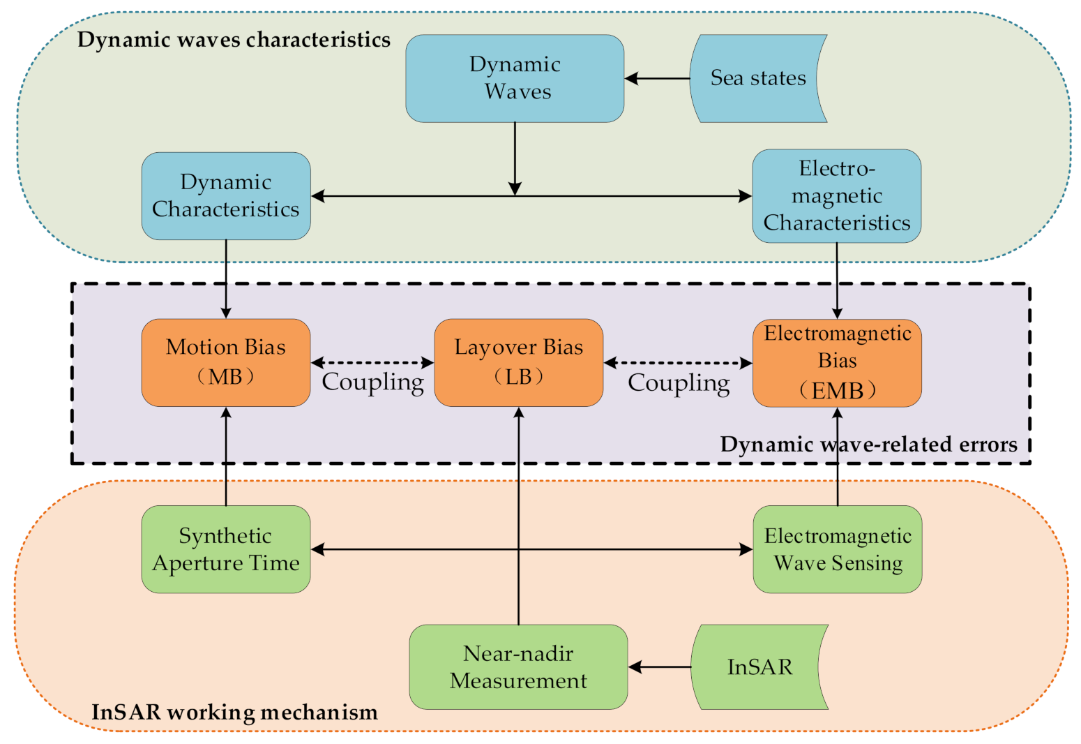
  • The mechanisms of the dynamic wave-related errors for InSAR ocean altimetry are analyzed, and a detailed numerical model is derived. Three key error sources are considered, MB, EMB, and LB, which means that the analysis is comprehensive. This is conducive to characterizing the impact of ocean waves on the SSH retrieved by InSAR.
  • Based on the wind-generated wave spectrum and three-scale second-order EM backscattering model, the dynamic wave-related errors of InSAR altimetry can be characterized for different radar parameters under various sea states, and this can be used for the error budget of InSAR altimetry under multiple scenarios.
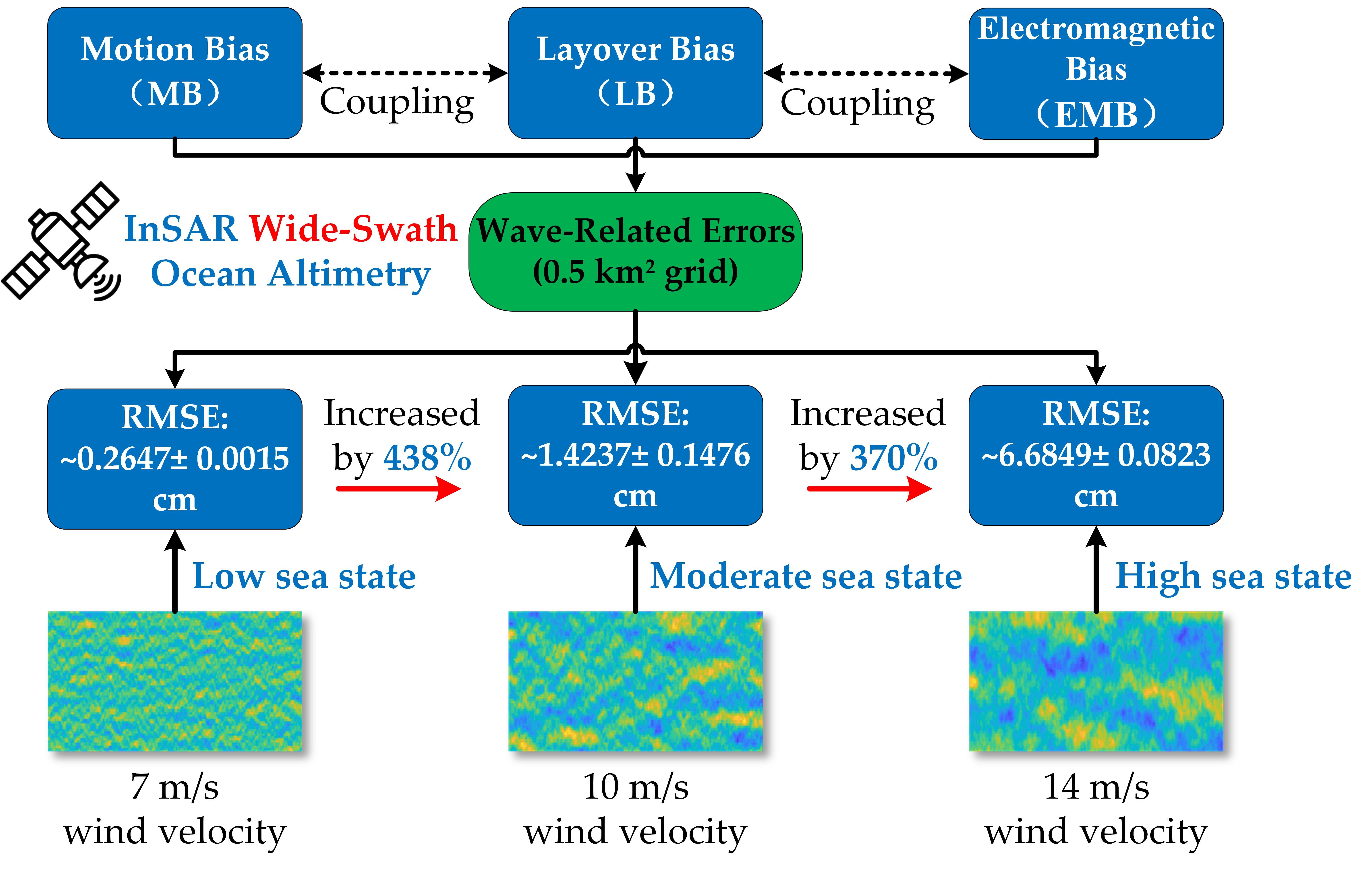
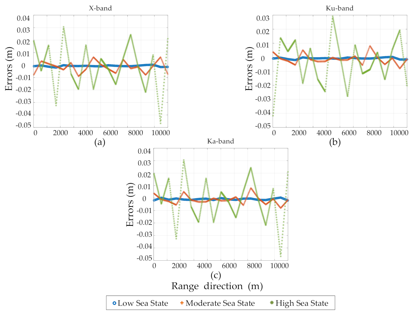
  • The RMSEs of three radar frequencies, X-band, Ku-band, and Ka-band, under three kinds of sea states are given; the results show that the frequencies have little impact on the dynamic wave-related errors, and the error compensation is needed for moderate and higher sea states for centimetric accuracy requirement. This can provide relevant suggestions for application scenarios and error compensation methods for future InSAR ocean altimetry.

2. Materials and Methods

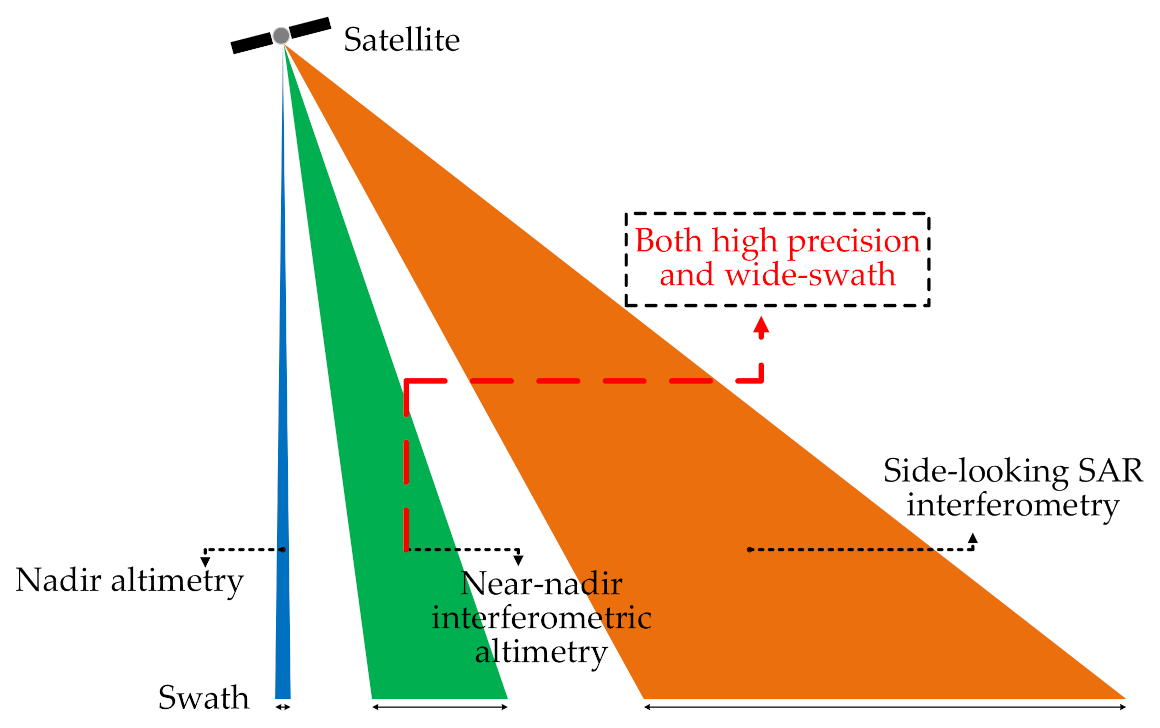
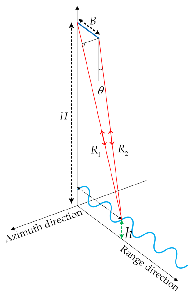
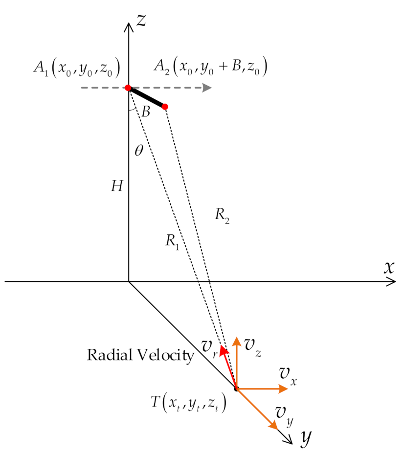
2.1. Principle of InSAR Altimetry

To characterize the altimetric errors due to the dynamic waves, the interference principle of InSAR is introduced first. The interferometric measurement concept could be approximately simplified as triangulation in Figure 2.
To simplify the calculation, it was assumed that the baseline angle is 0°; that is, the baseline is horizontal to the earth surface. The distance between two radar antennas (here referred to as “dual-transmit and dual-receive antenna”) is called the cross-track baseline B . For a typical point on the sea surface, R 1 and R 2 are the ranges between two antenna phase centers and the point target. The range difference between R 1 and R 2 is recorded by the interferometric phase difference φ between the two radar echoes. For two antennas, the received SAR signals can be expressed as:
S 1 ( t ) = ω 1 ( t ) exp j φ 1 R 1 = ω 1 ( t ) exp j 2 π λ · 2 R 1
S 2 ( t ) = ω 2 ( t ) exp j φ 2 R 2 = ω 2 ( t ) exp j 2 π λ · 2 R 2
where ω 1 t and ω 2 t are the amplitudes of the radar signals, and j represents the unit of imaginary numbers that j 2 = 1 . The relationship between interferometric phase difference φ and the slant ranges using the triangulation can be expressed by:
φ = φ 1 R 1 φ 2 R 2 = 2 π R 1 R 2 λ
where λ denotes the wavelength. The approximation is true that R 1 R 2 R 1 , and using the law of cosine, it could conclude that:
φ = 2 k R 1 k R 1 + R 2 k B sin ( θ )
where k is the EM wavenumber, which is related to the radar center carrier frequency and k = 2 π / λ . Since the baseline is horizontal, the look angle θ can be calculated as:
θ arcsin 16 π B 2 + 8 π R 1 ϕ λ ( φ λ ) 2 32 π 2 B R 1
From the phase measurement through the radar echoes, and with precise knowledge of the slant range R 1 , the final surface height h can be obtained by [13]:
h = H R 1 cos ( θ ) = H R 1 cos arcsin 16 π B 2 + 8 π R 1 φ λ ( φ λ ) 2 32 π 2 B R 1 H R 1 cos arcsin φ λ 4 π B
where H is the altitude of the antenna on the satellite platform. For ocean altimetry, the two antennas of InSAR should work simultaneously, and the imaging integration time should be short to avoid the decorrelation of the ocean [37]. The radar look angle θ is relatively small because the system operates at a near-nadir state for the high Signal-to-Noise Ratio (SNR) with strong reflection from the sea surface [38]. Moreover, the sensitivity of the interferometric phase can be increased in the small incidence angle so high precision can be achieved.

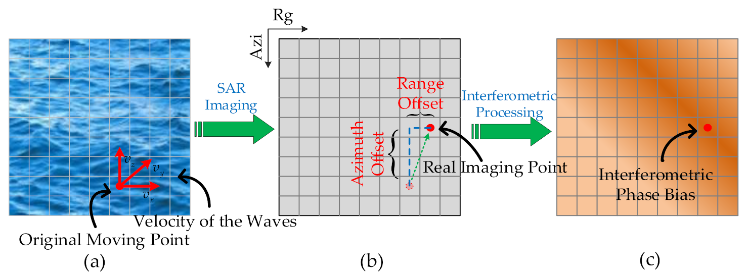
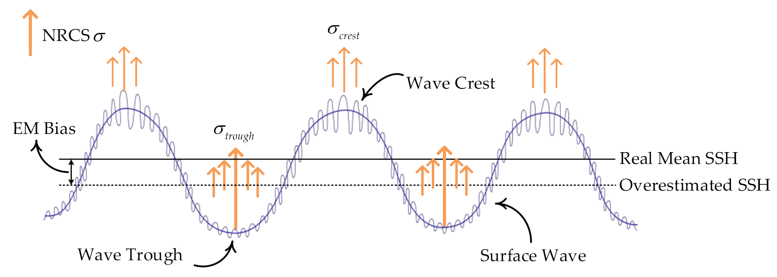
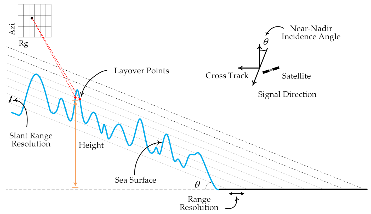
2.2. Mechanisms of the Dynamic Wave-Related Errors

Compared with the traditional pulse-limited nadir altimeter, the most significant difference for InSAR altimetry is the unique synthetic aperture time [23]. Therefore, the motion of the waves must be considered within the synthetic aperture period. Moreover, the wave crests and troughs have different strengths for EM scattering due to the hydrodynamic modulation effects, which will cause non-negligible range errors called EMB [32]. InSAR works in the microwave frequencies, so the EMB is consistent with traditional nadir altimeters, and this cannot be ignored. Additionally, for high-accuracy measurement, InSAR works in a near-nadir state; the layover phenomenon by the surface waves is profoundly serious at this time, and this will also cause related altimetric errors. Therefore, the dynamic wave-related errors for InSAR altimetry can be divided into three categories as shown in Figure 3, which are MB, EMB, and LB, separately. These three errors are all caused by waves that are coupled with one another and are closely related to the state of the waves.
The schematic diagram of the MB for InSAR altimetry can be expressed as seen in Figure 4. For the motion of the waves, it can generally be divided into surface motion and vertical motion, and surface motion can be divided into range motion and azimuth motion. These movements, respectively, correspond to the surface velocity and vertical velocity of the imaging targets. When SAR performs imaging, it assumes that the target is stationary. Due to the motion of the waves, the target in the final SAR image will shift, including azimuth offset δ x and slant range offset δ R . When the interferometric phase difference is used to perform the height inversion, the inevitable interferometric phase errors will be introduced due to the corresponding slant range offset δ R , and then the height offset δ h will be introduced. This will eventually lead to altimetric errors that cannot be ignored, which requires special attention.
Due to the motion of the target, the azimuth offset δ x in SAR image can be calculated as [21]:
δ x = v r v p R
where v p is the velocity of the satellite platform, v r is the radial velocity of the waves, R is the slant range between the radar and the target.
For the azimuth offset, the magnitude is relatively large, generally exceeding several azimuth resolutions [21]. The azimuth offset is well known for SAR ocean imaging, and many scientists have noticed this shift phenomenon, and it is called velocity bunching in wave imaging [22]. However, for the slant range offset, the magnitude is smaller than a range cell, and it is usually ignored in the SAR moving target process. Conversely, for high-accuracy height inversion, it is a decisive factor for the measurement and directly results in altimetric errors, and it cannot be ignored.
Through the principle of interferometric measurement, the slant range offset δ R can be calculated as:
δ R = f d λ v r R 2 v p 2 v r 2 R 2 v p 2
where f d is the Doppler central frequency of the InSAR. Based on δ R and the InSAR measurement geometric relationship, as shown in Figure A1 in Appendix A, the altimetric errors due to the offset in the slant range direction can be expressed as follows:
δ h δ R cos θ
After substituting Equation (8) into Equation (9), the altimetric errors can be conducted as:
δ h H λ f d v r 2 v p 2 H v r 2 2 v p 2
The detailed derivations of Equation (7), (8), and (10) are also given in Appendix A. Compared to the motion error theoretical model of SWOT project given by NASA [11]:
Δ h SWOT H v r v p α P i t c h
where the specific derivation of the parameter α p i t c h = λ f d 2 v p Hence, it is in good agreement with the first term in Equation (10), and this verifies the correctness of our model derivation. However, our model gives a more specific derivation, including the second term in Equation (10), and most effectively considers the effects of the second-order component. This is particularly important for centimeter-level accuracy requirements in InSAR measurement.
With regard to the influence of EMB on InSAR two-dimensional SSH measurement, different areas of the sea surface have different scattering intensity of EM waves. Due to the hydrodynamic modulation effects, the scattering intensity of wave troughs is greater than that of waves as σ t r o u g h > σ c r e s t , shown in Figure 5, which will have a weighting or modulation effect on the dynamic effects of the waves.
With regard to InSAR ocean altimetry, when a large number of scattering facets in the same cell are statistically superimposed, the statistical average of altimetric errors modulated by the normalized radar cross section (NRCS) σ can be expressed as:
δ h ¯ = δ h σ σ H λ f d v r σ 2 v p 2 σ H v r 2 σ 2 v p 2 σ
where 〈 〉 means the spatial average. At this time, the coupling of MB and EMB is included in Equation (12), and this provides a method for the consideration of InSAR EMB. Additionally, it is different from nadir altimeters; InSAR works in side-looking mode, and this causes intrinsic geometric distortions, such as foreshortening, shadow, or layover phenomena [34]. Because of the small incidence angle at near-nadir, the layover effect for InSAR SSH measurement is severe and cannot be ignored for high-accuracy requirement.
Figure 6 shows the simulated SSH under wind speed of 10m/s by Apel Wave Spectrum [39], and layover will occur when the wave slope is larger than the radar incidence angle. As shown in Figure 6, the red points are the radar sampling points, which have different heights, but are sampled into the same InSAR pixel unit. When the interference phase is extracted, the altimetric errors will be introduced. By the precise knowledge of the wave height and the radar parameters, such as the altitude of the satellite platform and the look angle, the layover effects can be calculated numerically [35]. In our analytical method, after setting the radar parameters, the layover effect is effectively quantified based on the preset geometry relationship.
The above are the theoretical basics for the analysis of InSAR dynamic wave-related errors, and the MB, EMB, and LB are all successfully analyzed and considered. Among them, these three kinds of errors are mutually coupled and need to be considered together in the final measurement results. Because of the mutual coupling effect, the possible correction of these wave-related errors should also be carried out at the same time.

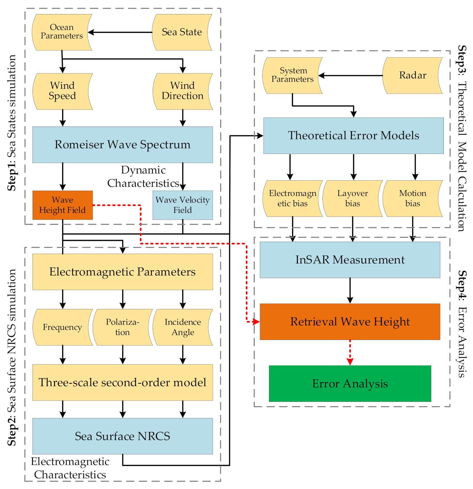
2.3. Analytical Methods

2.3.1. Romeiser Wave Spectrum

Wave spectrum is a common method for the numerical simulation of ocean scenes for different sea states, and a wind-generated wave spectrum proposed by Romeiser was used in this study. The Romeiser Wave Spectrum was modified based on the Apel Wave Spectrum and calibrated by actual ocean wave data, so that the reliability was higher [40,41]. The analytical expression of the Romeiser wave direction spectrum is as follows [40]:
ψ k w a v e , u 10 , ϕ = P L k w a v e , u 10 W H k w a v e u 10 u n β k w a v e k w a v e 4 S k w a v e , ϕ , u 10
where k w a v e is the wavenumber of ocean surface waves, u 10 represents the wind speed at the height of 10 meters above the ocean surface, and ϕ is the angle between wave and the wind direction. P L is a factor that describes a low wavenumber roll-off and Joint North Sea Wave Project (JONSWAP) peaking as a function of the wind speed. The expression of P L is as follows [39]:
P L = 0.00195 exp k p 2 k w a v e 2 + 0.53 exp k w a v e k p 2 0.32 k p
where k p = 1 2 g u 10 2 is the peak wavenumber and   g indicates the gravitational acceleration. β k w a v e is the corresponding wind speed exponent, and the optimization of β k w a v e after three iterations by Romeiser can be given as [40]:
β k w a v e = 1 exp k w a v e 2 k 1 2 exp k w a v e k 2 + 1 exp k w a v e k 3 exp k w a v e k 4 k 5 2
where the values of the parameters k 1 , k 2 , k 3 , k 4 ,   and k 5 , are 183, 3333, 33, 140, and 220 rad / m , respectively.   W H k w a v e is the shape analytic function [40]:
W H ( k w a v e ) = 1 + k w a v e k 6 7.2 0.5 1 + k w a v e k 7 2.2 1 + k w a v e k 8 3.2 2 exp k w a v e 2 k 9 2
where the values of the parameters k 6 , k 7 , k 8 , and k 9 are 280, 75, 1300, and 8885 rad / m , respectively. S k w a v e , ϕ , u 10 is the spreading function, and the expression is [40]:
S k w a v e , ϕ , u 10 = exp ϕ 2 2 ϑ 2
where ϑ   can be obtained from [39] as:
1 2 ϑ 2 = 0.14 + 0.5 1 exp k w a v e u 10 c 1 + 5 exp 2.5 2.6 I n u 10 u n 1.3 I n k w a v e k n
where c 1 = 400 rad / m ,   a n d   k n = 1   rad / m . After simulating the wave spectrum, the wave height fields (also known as water height fields) and wave velocity fields of the sea surface can be calculated. By Fourier decomposition, the two-dimensional wave height fields can be expressed as:
H ¯ w a v e x , y , t = 1 2 h w a v e ( k w a v e x , k w a v e y ) exp [ j ( k w a v e x x + k w a v e y y ω t ) + ϕ 0 ] d k w a v e x d k w a v e y + c . c . + H S S H x , y
The two-dimensional wave velocity fields introduced by the wind-generated waves can be expressed as (including along-track velocity, cross-track velocity, and vertical velocity):
V w a v e x x , y , t =                                     1 2 ω h w a v e ( k w a v e x , k w a v e y ) cos Φ k w a v e x , k w a v e y exp j k w a v e x x + k w a v e y y ω t + ϕ 0 d k w a v e x d k w a v e y + c . c .
V w a v e y x , y , t =                                     1 2 ω h w a v e ( k w a v e x , k w a v e y ) sin Φ k w a v e x , k w a v e y exp j k w a v e x x + k w a v e y y ω t + ϕ 0 d k w a v e x d k w a v e y + c . c .
V w a v e z x , y , t =                                     1 2 j ω h w a v e ( k w a v e x , k w a v e y ) exp j k w a v e x x + k w a v e y y ω t + ϕ 0 d k w a v e x d k w a v e y + c . c .
where h w a v e k w a v e x , k w a v e y is the ocean wave height spectrum, k w a v e x , k w a v e y are the wavenumber components of large-scale ocean waves parallel and perpendicular to the radar sight, ϕ 0 is the wave random phase, ω is the frequency of the surface wave, and c.c. means the complex conjugation of the former part that guarantees the entire expression to be a real value. H S S H x , y is the inherent height, which is the geophysical parameter we need to retrieve. V w a v e x x , y , t , V w a v e y x , y , t , and V w a v e z x , y , t are the wave velocities along three directions, and Φ k x w a v e , k y w a v e is the direction of the ocean wave propagation.

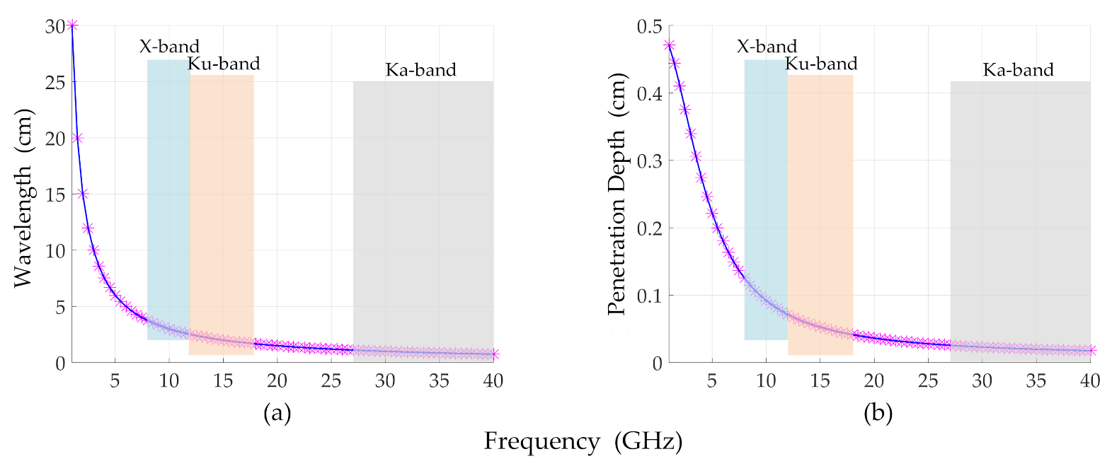
2.3.2. Three-Scale Second-Order Sea Surface Scattering Model

In the near-nadir situation, the quasi-specular scattering will dominate in the sea surface [42]. The three-scale composite model decomposes the scattering intensity into large-scale quasi-specular scattering, small-scale Bragg scattering, and intermediate-scale scattering [43]. Compared with the geometrical optics model, the radar incidence angle for the three-scale model is wider, and it is also suitable for small incidence angles, such as near-nadir InSAR altimetry. Therefore, a three-scale second-order sea surface scattering model was adopted for the NRCS numerical simulation in this study, and the sea surface time-varying NRCS can be expressed as [44]:
σ x , y , t = σ l x , y , t + σ i x , y , t + σ s x , y , t + σ 2 x , y , t
where σ l x , y , t , σ i x , y , t , and σ s x , y , t are the NRCS of large-scale waves, intermediate-scale waves, and small-scale waves, respectively. σ 2 x , y , t is the second-order scattering component. This model, used in our simulation, first divides surface waves into large-scale, intermediate-scale, and small-scale spectra based on the radar resolution and wavelength. Within this frame, the second-order scattering expressions are derived, and an analytic solution of hydrodynamic modulation function is developed according to weak hydrodynamic interaction theory. Additionally, tilt modulation is also implemented through the observation angle transform between nominal and local coordinate systems [44]. The scattering model fully considers the nonlinearity effects such as tilt and hydrodynamic modulation effects for SAR ocean imaging. This makes our simulated NRCS more consistent with real distributed SAR ocean imaging.
The complex scattering coefficient of a radar resolution in this study can be expressed as [45]:
ρ x , y , t = σ x , y , t exp j φ 0 + φ n x , y , t + 4 π D r x , y , t λ
where φ 0 is the initial random phase for sea surface scattering. φ n x , y , t is the decoherent random phase for the sea surface, which is caused by the random motion of the internal elements of the sea surface scattering surface. D r x , y , t is the time-varying radial displacement of the scattering surface element, which is caused by the motion of the ocean waves.

2.3.3. Analytical Flowchart

The analytical method flowchart proposed in this study is shown in Figure 7, where four necessary steps are involved. In the first step, the wave spectrum is used with the information of the sea states (including wind speed and wind direction). Then, the wave height field and wave velocity field due to the winds can be calculated by the spectrum decomposition. In the second step, based on the EM parameters of the InSAR, the two-dimensional ocean surface NRCS can be calculated by using a three-scale second-order sea surface scattering model. In the third step, the measurement errors are calculated based on the theoretical models; both EM characteristics and dynamic characteristics are taken into consideration, including MB, EMB, and LB. After the above three steps, based on the InSAR measurement geometry, the SSH can be retrieved with the impact of dynamic surface waves. By comparing the real wave height calculated by the wave spectrum, the dynamic wave-related altimetric errors can be characterized, and the analysis can be conducted. It should be noted that to better characterize the errors due to the dynamic waves, the rest of the system errors; random errors; and propagation errors, such as the baseline vibration, the orbit change, or the path delay, are ignored in our simulation.
For the spaceborne InSAR applied to ocean remote sensing, the preset single look resolution is not high, so the synthetic aperture integration time is relatively short [38,46]. In such a short SAR illumination time, the change of the sea surface NRCS with time can be neglected. Additionally, it can be assumed that the complex reflectivity of spatially separated sea surface cells is uncorrelated [47]. These are the basic assumptions for our experiments. As for vast ocean observation, multi-look averaging will be used to decrease the huge data rate [11]. The onboard processor (OBP) of SWOT will average the data down to a resolution of 500 m (along-track) × 500 m (cross-track) [38]. In this study, we also selected a 0.5 km2 grid averaging for two-dimensional resolution, so the spatial resolution of the final altimetric errors is 0.5 km2. The real sea states in the actual conditions are complicated (e.g., time-varying and space-varying wind waves and swells), and the simulation in this study only discusses wind waves in the open sea without considering swells. However, the altimetric error mechanisms for InSAR introduced by swells are the same as wind waves.

3. Results

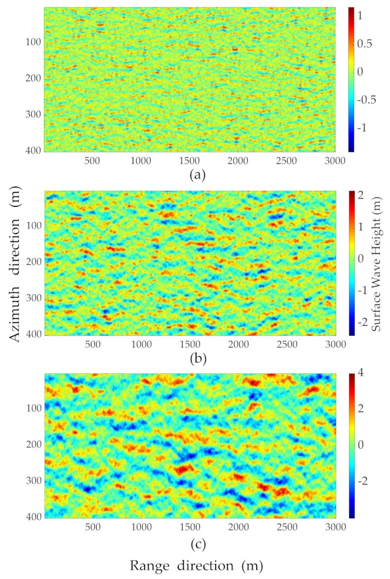
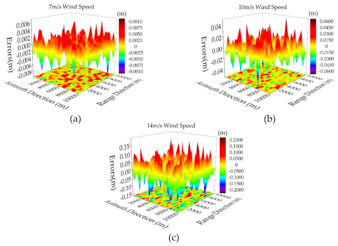
3.1. Stochastic Sea Scenes Simulation

The sea states in this study can be divided into three categories: low, moderate, and high sea states corresponding to wind speeds of 7, 10, and 14 m/s, respectively [23]. The two-dimensional surface wave height under different sea states in the space domain was generated based on the Romeiser Wave Spectrum, as shown in Figure 8, and the wind direction was along the radar range direction. It can be seen that as the sea state increases, the wave height of the sea surface gradually increases.
Based on the wave spectrum and EM scattering model, the sea surface NRCS of different frequencies can be calculated. The radar signals are mainly quasi-specular scattering of EM waves in this situation, and the NRCSs are relatively high for near-nadir incidences. The simulated NRCS values in our study are very close to those reported by altimeter actual data and SWOT airborne experimental data with a discrepancy within ~ 1 or 2 dB, and this also indicates the reliability of our analysis [38,48].
Figure 9 shows the partial two-dimensional ocean NRCS simulation results in the space domain under three frequencies of HH polarization based on three kinds of sea states. Among them, Figure 9a,d,g correspond to a wind speed of 7 m/s; Figure 9b,e,h correspond to a wind speed of 10 m/s; and Figure 9c,f,i correspond to a wind speed of 14 m/s. In Figure 9, we can see the texture of wind-generated waves clearly in the ocean scene, and as the wind speed increases, the waves become increasingly obvious. At the same time, the inhomogeneous reflectivity phenomenon caused by the hydrodynamic modulation effects on the sea surface can be clearly observed, in which the scattering intensity at the wave trough is greater than the wave crest.

3.2. Experimental Verification with SWOT Error Budget

To verify the correctness of the proposed analytical method, we conducted an error verification experiment based on the system parameters of the SWOT project and compared the numerical result with the SWOT motion error budget result given by NASA [11]. The system parameters are shown in Table 1, and they are based on the preset parameters of the forthcoming SWOT project (scheduled to be launched in 2022). Based on our analytical method as in Figure 7, the dynamic wave-related errors of InSAR can be calculated based on the SWOT parameters. It should be noted that this contrast experiment only considers the condition of the low sea states, and the SWH is ~2 m as in [11]. This is also the most common sea state in the ocean environment and has a certain degree of representativeness. In order to minimize the effect of the variation of the swath, the middle area (10,000 ×   10,000 m) of the swath was selected for our simulation.
Figure 10 is the three-dimensional distribution of the dynamic wave-related errors for InSAR altimetry based on the above-mentioned parameters of SWOT. As we can see, under the resolution of the 0.5 km2 grid, the level of the errors under low sea states is relatively smaller. By statistical analysis, the RMSE can be calculated as shown in Table 2. The RMSE based on the proposed method is 0.2486 cm; meanwhile, the RMSE introduced by wave motion given by NASA for SWOT is 0.2470 cm [11]. The results of the two experiments are well-matched, indicating the correctness and reliability of our analytical method. At the same time, the small difference may be that we consider the coupling of EMB and LB from the waves in our experiment. This also makes the simulation results closer to the actual InSAR stochastic ocean measurement scenarios.

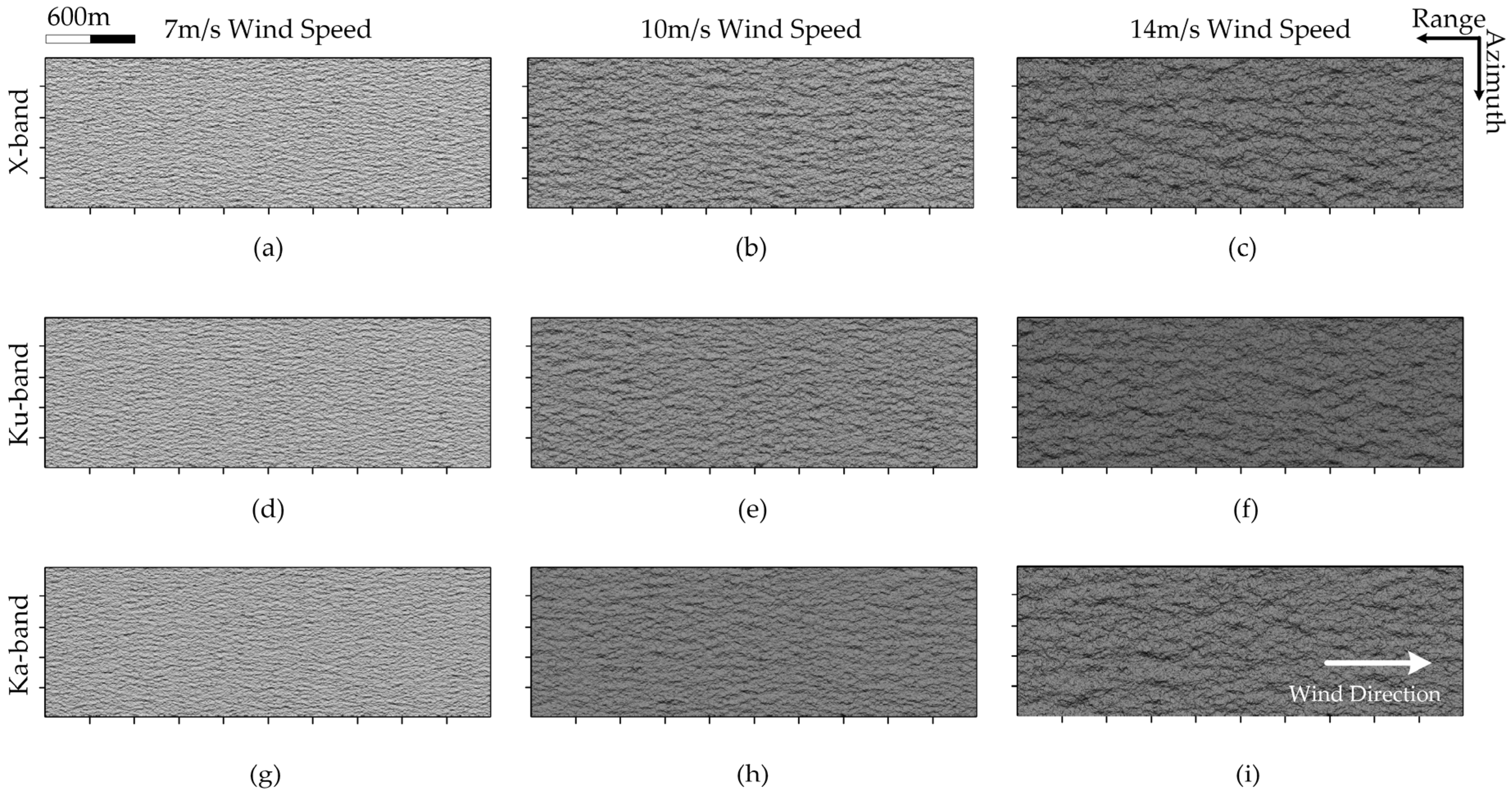
3.3. Experiments under Multiple Scenarios

Instead of analysis for a typical project such as SWOT, the proposed method can be applied to different radar parameters, such as multi-frequencies (e.g., C-band, X-band, Ku-band, or Ka-band) under various sea states (e.g., wind speed ranging from 1 to 20 m/s). Figure 11 reveals the wavelength distribution of different EM frequencies and their penetration ability into the sea surface. It can be observed that as the wavelength becomes shorter, the penetration into the sea surface becomes worse. Moreover, different frequencies have different sensitivity to the sea surface; the short wavelength is more sensitive to small-scale phenomena on the sea surface, and the phase information of the InSAR echoes is more accurate [38]. This will cause differences in the measurement accuracy of InSAR altimetry and is a factor to be considered.
Additionally, sea states have a great influence on the accuracy of the SSH retrieved by InSAR [28]. Based on the simulated wave spectrum, the wave height field and wave velocity field of different sea states can be calculated. Therefore, the dynamic wave-related errors of InSAR altimetry can be characterized under different sea states in our method. We analyzed these errors in three kinds of frequencies, X-band, Ku-band, and Ka-band, under three kinds of sea states. The system simulation parameters are shown in Table 3 as common parameters of spaceborne ocean SAR. The incidence angle is 4° at the near range and 4.7° at the far range, which indicates the typical situation as near-nadir [23].
It is worth noting that in the process of our simulation, the influence of the layover effect is included based on the InSAR measurement geometry and wave height field. Moreover, the influence of EMB is considered with the simulation of the two-dimensional sea surface NRCS. The simulated dynamic wave-related errors of InSAR altimetry are given separately in Figure A2, Figure A3, and Figure A4 in Appendix B. It can be observed that the distribution of these errors is random like waves. Furthermore, as the wind speed increases, the value of the dynamic wave-related errors also increases. Figure 12 shows the comparisons of the dynamic wave-related errors under different sea states along the range direction. It can be clearly seen that as the sea state increases, the magnitude of the wave-related errors of InSAR altimetry becomes larger.
Table 4 shows the statistical results of the dynamic wave-related errors under multiple wavebands, and it is possible to obtain the RMSEs in three kinds of frequencies under three sea states. The RMSEs under different sea states are 0.2647 ± 0.0015 cm, 1.4237 ± 0.1476 cm, and 6.6849 ±   0.0823 cm, respectively. It can be observed that under the same sea states, the RMSEs in different frequencies are relatively similar, with little difference. Among them, the average fluctuation range of RMSE for three wavebands is ± 0.58% (low sea states), ± 10.37% (moderate sea states), and ± 1.23% (high sea states), respectively. However, from low sea states to moderate sea states, the average RMSE increases by 438% (from 0.2647 to 1.4237 cm) for three wavebands. From moderate sea states to high sea states, the average RMSE increases by 370% (from 1.4237 to 6.6849 cm) for three wavebands. It can be seen that this type of error is very sensitive to sea states, and the magnitude increases significantly with the increase in sea states.

4. Discussion

Compared with the traditional nadir altimeter, spaceborne near-nadir InSAR can improve the spatial–temporal resolution of SSH observations and effectively make up for the lack of existing ocean observation tools [37]. Currently, many international institutions begin to develop their own wide-swath InSAR altimetry satellites (e.g., SWOT by the NASA [18], InIRA by the NSSCCAS [25], and Guanlan by the NLMSTC [28]), and this is the most promising instrument for future ocean topography measurement. To fulfill the targeted measurement accuracy for ocean scientific research, the error budget and analysis of InSAR altimetry are relatively essential at present. For the conventional nadir altimeter, there are many in-depth investigations on its error mechanisms and compensation methods, whether theoretical or empirical [29,30]. Among them, the errors caused by the waves, also known as SSB, have become the most important source of altimetric errors [32]. Through the valid calibration of SSB, the SSH measurement accuracy by the nadir altimeter can reach an extremely high level of about 2 cm and has been wildly used for large-scale OST observation [5,6,49]. Therefore, it is also imperative to study the wave-related error mechanisms of InSAR altimetry. Inspired by the wave-related errors for the nadir altimeter (e.g., EMB, skewness bias, and tracker bias [29]), the wave-related errors for InSAR can be divided as MB, EMB, and LB, respectively. This is why we conducted this study and investigated the impact of wave-related errors of InSAR ocean altimetry under multiple sea states.

4.1. Suggestions for the System Design of InSAR Altimetry

For traditional nadir altimeters, such as Poseidon, the frequencies are in the Ku-band [29]. For the Jason series, to correct the atmosphere delay errors more accurately, a dual-frequency working system is adopted [6]. According to the above experimental results for different frequencies (Table 4), it can be seen that the dynamic wave-related errors are not sensitive to InSAR frequencies; the RMSEs of different frequencies are not very different. This is consistent with the actual data of conventional nadir altimeters, and the magnitudes of the measured SSB between different radar frequencies are similar (e.g., Ku-band of TOPEX and C-band of Jason-1 [32]). This means that the choice of wavebands for InSAR SSH measurement should more thoroughly consider the antenna design or propagation errors. As is well known, the SWOT project proposed Ka-band for interferometry [38]; however, the InIRA on the Tiangong II laboratory adopts Ku-band antennas [50]. For Guanlan’s IRA project, a dual-frequency system is used, which includes both Ku and Ka-bands antennas [28]. Compared with the Ku-band, the ionosphere has a smaller influence on the Ka-band, but rainy weather has a greater impact on the Ka-band [11,15]. However, the EM wavelength of the ka-band is shorter, which can better measure the small-scale processes of the ocean surface [38]. Since the frequency is not sensitive to dynamic wave-related errors of InSAR altimetry, the choice of future wavebands has greater flexibility for different ocean scientific requirements.

4.2. Possible Method to Reduce Dynamic Wave-Related Errors

Centimeter-level accuracy of SSH measurement is required for applications such as gravity anomaly or geostrophic currents observation [10]. For the dynamic wave-related errors of InSAR altimetry, the RMSE is under a millimeter scale of ~ 0.2647 cm for low sea states (Table 4). This shows that this type of error can be ignored under low sea states in most calm conditions with small wave heights and wave slopes for centimetric accuracy. Therefore, for Ka-band SWOT and Ku-band InIRA, the dynamic wave-related errors can be ignored under low sea states, and this is not an important source of altimetric errors. However, when moderate or higher sea states occur, the RMSE is under a centimeter scale of ~ 1.4237 cm or higher (Table 4), which means the errors cannot be ignored, and the error compensation method is necessary for centimeter-level accuracy requirements. Thus, the compensation methods for these errors under moderate and higher sea states are a problem that must be solved. Here, we provide a possible approach to reduce the wave-related altimetric errors based on the derived theoretical model. Through the theoretical derivation in Equation (12), altimetric errors caused by the wave motion are not only related to the sea state, such as the radial velocity of the waves, but also to the radar system parameters, such as Doppler central frequency, the altitude, and velocity of the satellite platform. Thus, the zero Doppler technology as the yaw steering method of the satellite could be used [51]. In this way, only the second-order term of the altimetric errors is left, and the influence of the dynamic waves can be reduced as much as possible.

4.3. Limitations and Future Directions

The features of ocean waves are very complex, and it is very difficult to characterize all the effects of ocean waves on InSAR altimetry. Most of the previous studies consider the different effects of ocean waves separately. Peral et al. [18] analyze several effects, such as volumetric decorrelation, backscattering modulation, and aliasing of the waves, separately. Additionally, some useful conclusions are given based on the parameters of the SWOT project, for example, the EMB could be estimated by the usage of the wave spectrum. Bai et al. [28] study the effects of layover and velocity bunching for the Guanlan project separately, and a large number of simulation results are given. The results show that layover and velocity bunching have different impacts on the final measurement performance. Our study considers multiple effects, such as MB, EMB, and LB of the waves and couples them to evaluate the final impact. Thus, the results obtained in this study are closer to the real measurement scene as InSAR ocean altimetry. However, there are still fewer limitations for the study in this paper. First, the current missions of InSAR ocean altimetry satellite are still in a pre-research state in most countries, and the actual SSH data by spaceborne InSAR are scarce [18,28]. Although some airborne experiments have been carried out (e.g., AirSWOT for SWOT [38] and AIRAS for Guanlan [27]), the quality of the measured data is not high enough for accuracy analysis in centimeters. Therefore, the theoretical error model in this paper is only compared with the result given by the SWOT team in [11], and the follow-up needs to be verified by measured spaceborne InSAR data. Second, the real sea states are very complicated (including both the open sea and coastal zones), but the wind-generated wave spectrum can only simulate the condition of the fully developed open sea [41,42]. However, the measurement of coastal zones is also an issue that needs to be considered for InSAR altimetry [52]. The analysis of the altimetric accuracy in the coastal zones is also a factor that needs to be addressed in the future.

5. Conclusions

Near-nadir InSAR has huge potential to measure the SSH with high accuracy based on a finer spatial resolution that has never been resolved before. The study and analysis of the errors introduced by the dynamic ocean waves are necessary steps to achieve the targeted accuracy for InSAR ocean altimetry. An analytical method for wave-related errors of InSAR altimetry is proposed in this paper based on the wave spectrum and EM scattering model, and the error numerical model was derived. The proposed error analytical method takes into account both the ocean characteristics and the InSAR working characteristics, which can better simulate the distribution of errors as in the actual ocean scene. The simulated RMSE is validated with the SWOT error budget result, and the results are in good agreement. In addition to the analysis of typical projects, such as SWOT or InIRA, more simulations can be carried out for different radar parameters under various sea states based on our analytical method. The simulation experiments were conducted under multiple scenarios, and the RMSEs for three radar frequencies under three kinds of sea states are given. The results obtained in this study demonstrate that the magnitude of dynamic wave-related errors of InSAR is in the order of millimeters as ~ 0.2647 cm in low sea states, but in the order of centimeters as ~ 1.4237 to ~ 6.6849 cm under moderate to higher sea states.
To the best of our knowledge, this is the first numerical study to analyze the dynamic wave-related errors that contain multiple coupling sources, including MB, EMB, and LB, for InSAR SSH measurement and compare the RMSEs under different radar parameters and sea states. It is worth mentioning that our method can simulate more situations, such as different velocity or altitude of the InSAR platform, and can be used to demonstrate the radar system parameters in the pre-research phase. Future work will concern the development of more accurate wave spectrum and EM scattering models for near-nadir InSAR. Related water tank experiments are also in the design stage and will be carried out in the future to refine the theoretical error model.

Author Contributions

Conceptualization, Y.C. and M.H.; methodology, Y.C., M.H. and T.D.; software, Y.C., Y.Z. and C.W.; validation, Y.C., C.W. and T.D.; formal analysis, Y.C., Y.Z. and C.W.; investigation, Y.C., Y.Z. and C.W.; resources, M.H. and T.D.; data curation, Y.Z., M.H. and T.D.; writing—original draft preparation, Y.C. and T.D.; writing—review and editing, Y.C., T.D. and M.H.; visualization, Y.C., C.W. and T.D.; supervision, T.D. and M.H.; project administration, T.D. and M.H.; funding acquisition, T.D. and M.H. All authors have read and agreed to the published version of the manuscript.

Funding

This work was supported by the Director’s Foundation of Institute of Microelectronics, Chinese Academy of Sciences under Grant no. E0518101.

Acknowledgments

We thank the editors who handled the manuscript and the anonymous reviewers for their comments towards improving this manuscript. We thank Wang Xiaoqing and Huang Haifeng from Sun Yat-sen University for their helpful discussions on ocean scenes simulation. Moreover, we express gratitude to Kong Weiya from Qian Xuesen Laboratory of Space and Technology for his helpful suggestions on this paper.

Conflicts of Interest

The authors declare no conflict of interest.

Abbreviations

AbbreviationThe full name
SSHSea Surface Height
InSARInterferometric Synthetic Aperture Radar
NRCSNormalized Radar Cross Section
RMSERoot-Mean-Square Error
NASANational Aeronautics and Space Administration
SWOTSurface Water and Ocean Topography
TOPEXTopography Experiment
CryoSat-2Cryosphere Satellite 2
Jason-CSJason Continuity of Services Satellite
HY-2A/B/CHaiyang 2A, 2B, and 3C Satellites
OSTOcean Surface Topography
IRAInterferometric Radar Altimeter
SRTMShuttle Radar Topography Mission
EMBElectromagnetic Bias
KaRInKa-band Radar Interferometer
InIRAInterferometric Imaging Radar Altimeter
NSSCCASNational Space Science Center of Chinese Academy of Sciences
SSBSea State Bias
NLMSTCNational Laboratory for Marine Science and Technology of China
SWHSignificant Wave Height
PODPrecision Orbit Determination
LBLayover Bias
MBMotion Bias
SNRSignal-to-Noise Ratio
JONSWAPJoint North Sea Wave Project
OBPOnboard Processor
AIRASAirborne Interferometric Radar Altimeter System

Appendix A. Detailed Derivation of the Motion Bias

Figure A1 shows a schematic diagram of the geometric relationship for InSAR measurement of a point target with motion.   A 1 x 0 , y 0 , z 0 and A 2 x 0 , y 0 + B , z 0 are the coordinates of the two radar antennas. T x t , y t , z t is the coordinate of the moving point target on the sea surface, v x is the alone-tracker velocity of the point target, v y is the cross-track velocity and the vertical velocity is v z .
Figure A1. Diagram of the motion effect for InSAR measurement. The baseline direction is perpendicular to the azimuth direction, and it is assumed that the baseline angle is 0° to better characterize the motion bias.
Remotesensing 13 00986 g0a1
Due to the motion of the target, the time-varying slant range can be expressed as:
R 1 = x 0 + v p t x t + v x t 2 + y 0 y t + v y t 2 + z 0 z t + v z t 2
R 2 = x 0 + v p t x t + v x t 2 + y 0 + B y t + v y t 2 + z 0 z t + v z t 2
where t is the synthetic aperture integration time. Here, let R 1 be an example, and it can be expressed as:
R 1 2 = x 0 x t 2 + y 0 y t 2 + z 0 z t 2 + v p 2 + v x 2 + v y 2 + v z 2 2 v p v x t 2 + 2 x 0 x t v p v x 2 y 0 y t v y 2 z 0 z t v z t
The constant term R c o n s in Equation (A3) is:
R c o n s 2 = x 0 x t 2 + y 0 y t 2 + z 0 z t 2
The variable term R v a r in Equation (A3) which contains the second-order term and the first-order term is:
R v a r 2 = v p 2 + v x 2 + v y 2 + v z 2 2 v p v x t 2 + 2 x 0 x t v p v x 2 y 0 y t v y z z 0 z t v z t
For R 1 = R c o n s 2 + R v a r 2 , the Taylor’s first-order expansion of R 1 can be expressed as:
R 1 = R c o n s 1 + R v a r 2 R c o n s 2 R c o n s + R v a r 2 2 R c o n s
where R 1 R c o n s + R v a r 2 2 R c o n s = R c o n s + ξ 2 t 2 + ξ 1 t 2 R c o n s , and ξ 2 represents the coefficient of the second-order term, and ξ 1 represents the coefficient of the first-order term:
ξ 2 = v p 2 + v x 2 + v y 2 + v z 2 2 v p v x
ξ 1 = 2 x 0 x t v p v x 2 y 0 y t v y 2 z 0 z t v z
Therefore, the SAR echo S 1 t from antennas A 1 can be expressed as:
S 1 t = ω t exp j π 4 R c o n s λ + 2 ξ 2 · t 2 λ R c o n s + 2 ξ 1 · t λ R c o n s
S 1 t can be regarded as a chirp signal, K = 2 ξ 2 λ R c o n s is the frequency modulation slope, and   f d = ξ 1 λ R c o n s is the Doppler centroid frequency. So, Equation (A9) can be simplified as:
S 1 t = ω t exp j π 4 R c o n s λ + K t 2 + 2 f d t
when SAR imaging is performed, the target is assumed to be stationary. The signal can be processed by match filtering; the first-order term and the constant term of Equation (A10) will be eliminated. The real imaging point coordinate and offsets due to the motion can be obtained:
x t = x 0 x 0 x t v p v x y 0 y t v y z 0 z t v z v p
Δ x = x t x t = v r v p R c o n s
y t = y t + Δ x 2 x 0 x t Δ x 2 z 0 z t z t 2 y 0 y t
Δ y = y t y t = Δ x 2 x 0 x t Δ x 2 z 0 z t z t 2 y 0 y t
T * x t * , y t * is the real imaging coordinates due to the motion, and Δ x ,   Δ y are the offsets in azimuth direction and range direction, respectively.
Further calculations are available:
Δ y x 0 x t y 0 y t Δ x Δ x 2 2 y 0 y t z 0 z t y 0 y t = R c o n s λ f d y 0 y t · v r R c o n s 2 v p 2 v r 2 R c o n s 2 2 v p 2 y 0 y t z 0 z t y 0 y t
Based on   Δ x and Δ y , the offset in slant range Δ R 1 can be derived as:
Δ R 1 = x 0 x t Δ x R c o n s f d λ v r R c o n s 2 v p 2
In the same way, Δ R 2 can be obtained, then the interferometric phase φ can be calculated as:
φ π 2 16 exp 8 j π λ y 0 y t B R 1
The look angle θ related to the interferometric phase can be approximated as:
cos θ = x 0 x t 2 + z 0 2 R c o n s z 0 z t R c o n s
Thus, the altimetric errors due to the motion can be expressed as:
Δ h Δ R 1 cos θ = H λ f d v r 2 v p 2 H v r 2 2 v p 2

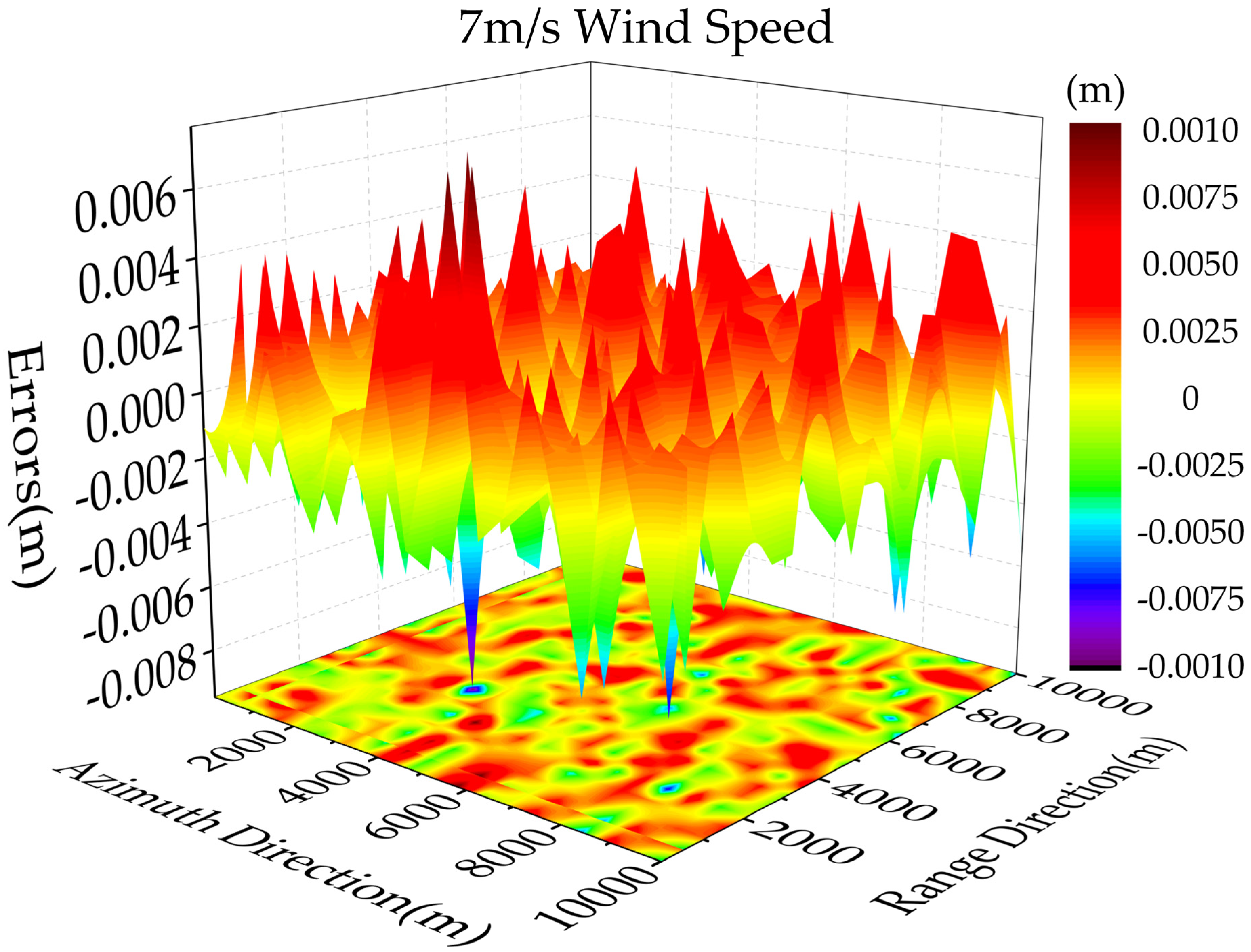
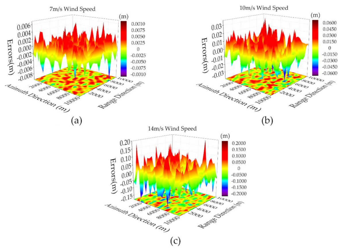
Appendix B. Three-Dimensional Distribution of the Simulated Dynamic Wave-Related Errors

Figure A2. Three-dimensional distribution of the dynamic wave-related errors for X-band InSAR altimetry under three different sea states: (a) low sea state; (b) moderate sea state; (c) high sea state.
Remotesensing 13 00986 g0a2
Figure A3. Three-dimensional distribution of the dynamic wave-related errors for Ku-band InSAR altimetry under three different sea states: (a) low sea state; (b) moderate sea state; (c) high sea state.
Remotesensing 13 00986 g0a3
Figure A4. Three-dimensional distribution of the dynamic wave-related errors for Ka-band InSAR altimetry under three different sea states: (a) low sea state; (b) moderate sea state; (c) high sea state.
Remotesensing 13 00986 g0a4

References

  1. Fu, L.-L.; Chelton, D.B.; Le Traon, P.-Y.; Morrow, R. Eddy dynamics from satellite altimetry. Oceanography 2010, 23, 15–24. [Google Scholar] [CrossRef] [Green Version]
  2. Chelton, D.; Ries, J.; Haines, B.; Fu, L.; Callahan, P. Satellite Altimetry and Earth Sciences: A Handbook of Techniques and Applications; Academic Press: San Diego, CA, USA, 2001; pp. 1–3. [Google Scholar]
  3. Legeais, J.; Ablain, M.; Zawadzki, L. An improved and homogeneous altimeter sea level record from the ESA Climate Change Initiative. Earth Syst. Sci. Data. 2018, 10, 281–301. [Google Scholar] [CrossRef] [Green Version]
  4. Ablain, M.; Meyssignac, B.; Zawadzki, L. Uncertainty in satellite estimates of global mean sea-level changes, trend and acceleration. Earth Syst. Sci. Data 2019, 11, 1189–1202. [Google Scholar] [CrossRef] [Green Version]
  5. Scharroo, R.; Bonekamp, H.; Ponsard, C.; Parisot, F.; von Engeln, A.; Tahtadjiev, M.; de Vriendt, K.; Montagner, F. Jason continuity of services: Continuing the Jason altimeter data records as Copernicus Sentinel-6. Ocean Sci. 2016, 12, 471–479. [Google Scholar] [CrossRef] [Green Version]
  6. Jia, Y.; Yang, J.; Lin, M.; Zhang, Y.; Ma, C.; Fan, C. Global assessments of the HY-2B measurements and cross-calibrations with Jason-3. Remote Sens. 2020, 12, 2470. [Google Scholar] [CrossRef]
  7. Chen, G.; Tang, J.; Zhao, C.; Wu, S.; Yu, F.; Ma, C.; Xu, Y.; Chen, W.; Zhang, Y.; Liu, J.; et al. Concept design of the “Guanlan” science mission: China’s novel contribution to space oceanography. Front. Mar. Sci. 2019, 6, 194. [Google Scholar] [CrossRef] [Green Version]
  8. Archer, M.; Li, Z.; Fu, L. Increasing the space-time resolution of mapped sea surface height from altimetry. J. Geophys. Res. Ocean. 2020, 124, 1–18. [Google Scholar] [CrossRef]
  9. Scharffenberg, M.; Stammer, D. Time-space sampling-related uncertainties of altimetric Global Mean Sea Level estimates. J. Geophys. Res. Ocean. 2019, 124, 7743–7755. [Google Scholar] [CrossRef] [Green Version]
  10. Kong, W.; Liu, B.; Sui, X.; Zhang, R.; Sun, J. Ocean surface topography altimetry by large baseline cross-interferometry from satellite formation. Remote Sens. 2020, 12, 3519. [Google Scholar] [CrossRef]
  11. Esteban-Fernandez, D. SWOT Project Mission Performance and Error Budget Document. JPL D-79084; 2017; pp. 19–73. Available online: https://pdms.jpl.nasa.gov/ (accessed on 23 September 2020).
  12. Quartly, G.D.; Chen, G.; Nencioli, F.; Morrow, R.; Picot, N. An overview of requirements, procedures and current advances in the calibration/validation of radar altimeters. Remote Sens. 2021, 13, 125. [Google Scholar] [CrossRef]
  13. Rodriguez, E.; Martin, J.M. Theory and design of interferometric synthetic aperture radars. Radar Signal Process. IEE Proc. 1992, 39, 147–159. [Google Scholar] [CrossRef]
  14. Ansari, H.; Zan, F.; Parizzi, A. Study of systematic bias in measuring surface deformation with SAR interferometry. IEEE Trans. Geosci. Remote Sens. 2021, 59, 1285–1301. [Google Scholar] [CrossRef]
  15. Liu, Z.; Zhou, C.; Fu, H.; Zhu, J.; Zuo, T. A framework for correcting ionospheric artifacts and atmospheric effects to generate high accuracy InSAR DEM. Remote Sens. 2020, 12, 318. [Google Scholar] [CrossRef] [Green Version]
  16. Rodriguez, E.; Morris, C.S.; Belz, E.J. A global assessment of SRTM performance. Photogramm. Eng. Remote Sens. 2006, 72, 249–260. [Google Scholar] [CrossRef] [Green Version]
  17. Pinel, S.; Bonnet, M.; Silva, J.; Moreira, D.; Calmant, S.; Satgé, F.; Seyler, F. Correction of interferometric and vegetation biases in the SRTMGL1 spaceborne DEM with hydrological conditioning towards improved hydrodynamics modeling in the Amazon Basin. Remote Sens. 2015, 7, 16108–16130. [Google Scholar] [CrossRef] [Green Version]
  18. Peral, E.; Rodríguez, E.; Esteban-Fernández, D. Impact of surface waves on SWOT’s projected ocean accuracy. Remote Sens. 2015, 7, 14509–14529. [Google Scholar] [CrossRef] [Green Version]
  19. Chen, Y.; Huang, M.; Wang, X.; Huang, H. Error analysis of dynamic sea surface height measurement by near-nadir interferometric SAR. J. Electron. Inf. Technol. 2020, 42, 547–554. [Google Scholar]
  20. Reale, F.; Dentale, F.; Carratelli, E.P.; Fenoglio-Marc, L. Influence of sea state on sea surface height oscillation from doppler altimeter measurements in the North Sea. Remote Sens. 2018, 10, 1100. [Google Scholar] [CrossRef] [Green Version]
  21. Alpers, W.; Rufenach, C.L. The effect of orbital motions on synthetic aperture radar imagery of ocean waves. IEEE Trans. Antenn. Propag. 1979, 27, 685–690. [Google Scholar] [CrossRef]
  22. Yoshida, T. Numerical research on clear imaging of azimuth-traveling ocean waves in SAR images. Radio Sci. 2016, 51, 989–998. [Google Scholar] [CrossRef] [Green Version]
  23. Chen, Y.; Wang, X.; Huang, M.; Feng, J.; Huang, H.; Chen, G.; Chen, Z. Analysis of the sea state bias in interferometric radar altimeter. In Proceedings of the China International SAR Symposium, Shanghai, China, 11 October 2018; pp. 1–7. [Google Scholar]
  24. Ma, C.; Guo, X.; Zhang, H.; Di, J.; Chen, G. An investigation of the influences of SWOT sampling and errors on ocean eddy observation. Remote Sens. 2020, 12, 2682. [Google Scholar] [CrossRef]
  25. Kong, W.; Chong, J.; Tan, H. Performance analysis of ocean surface topography altimetry by Ku-Band near-nadir interferometric SAR. Remote Sens. 2017, 9, 933. [Google Scholar] [CrossRef] [Green Version]
  26. Ren, L.; Yang, J.; Dong, X.; Zhang, Y.; Jia, Y. Preliminary evaluation and correction of sea surface height from Chinese Tiangong-2 interferometric imaging radar altimeter. Remote Sens. 2020, 12, 2496. [Google Scholar] [CrossRef]
  27. Yang, L.; Xu, Y.; Zhou, X.; Zhu, L.; Jiang, Q.; Sun, H.; Chen, G.; Wang, P.; Mertikas, S.; Fu, Y.; et al. Calibration of an airborne interferometric radar altimeter over the Qingdao Coast Sea, China. Remote Sens. 2020, 12, 1651. [Google Scholar] [CrossRef]
  28. Bai, Y.; Wang, Y.; Zhang, Y.; Zhao, C.; Chen, G. Impact of ocean waves on Guanlan’s IRA measurement error. Remote Sens. 2020, 12, 1534. [Google Scholar] [CrossRef]
  29. Gaspar, P.; Ogor, F.; Le Traon, P.Y.; Zanife, O.Z. Estimating the sea state bias of the TOPEX and Poseidon altimeters from crossover differences. J. Geophys. Res. Ocean. 1994, 99, 24981–24994. [Google Scholar] [CrossRef]
  30. Passaro, M.; Nadzir, Z.A.; Quartly, G.D. Improving the precision of sea level data from satellite altimetry with high-frequency and regional sea state bias corrections. Remote Sens. Environ. 2018, 218, 245–254. [Google Scholar] [CrossRef] [Green Version]
  31. Rodriguez, E.; Pollard, B.; Martin, J. Wide-swath ocean altimetry using radar interferometry. IEEE Trans. Geosci. Remote Sens. 1999, 37, 624–626. Available online: http://hdl.handle.net/2014/17962 (accessed on 28 October 2020).
  32. Gommenginger, C.; Srokosz, M. An investigation of altimeter sea state bias theories. J. Geophys. Res. Oceans 2003, 108, 1–13. [Google Scholar] [CrossRef]
  33. Reale, F.; Dentale, F.; Carratelli, E.P. Numerical simulation of whitecaps and foam effects on satellite altimeter response. Remote Sens. 2014, 6, 3681–3692. [Google Scholar] [CrossRef] [Green Version]
  34. Gower, J. Layover in satellite radar images of ocean waves. J. Geophys. Res. Oceans 1983, 88, 7719–7720. [Google Scholar] [CrossRef]
  35. Durand, M.; Chen, C.; Frasson, R.; Pavelsky, T.; Williams, B.; Yang, X.; Fore, A. How will radar layover impact SWOT measurements of water surface elevation and slope, and estimates of river discharge? Remote Sens. Environ. 2020, 247, 1–15. [Google Scholar] [CrossRef]
  36. Moreira, A.; Prats-Iraola, P.; Younis, M.; Krieger, G.; Hajnsek, I.; Papathanassiou, K.P. A tutorial on synthetic aperture radar. IEEE Geosci. Remote Sens. Mag. 2013, 1, 6–43. [Google Scholar] [CrossRef] [Green Version]
  37. Fu, L.L.; Ubelmann, C. On the transition from profile altimeter to swath altimeter for observing global ocean surface topography. J. Atmos. Ocean. Technol. 2014, 31, 560–568. [Google Scholar] [CrossRef]
  38. Fjørtoft, R.; Gaudin, J.-M.; Pourthié, N.; Lalaurie, J.-C.; Mallet, A.; Nouvel, J.-F.; Martinot-Lagarde, J.; Oriot, H.; Borderies, P.; Ruiz, C. KaRIn on SWOT: Characteristics of near-nadir Ka-band interferometric SAR imagery. IEEE Trans. Geosci. Remote Sens. 2013, 52, 2172–2185. [Google Scholar] [CrossRef]
  39. Apel, J. An improved model of the ocean surface wave vector spectrum and its effects on radar backscatter. J. Geophys. Res. Ocean. 1994, 99, 16269–16291. [Google Scholar] [CrossRef]
  40. Romeiser, R.; Alpers, W.; Wismann, V. An improved composite surface model for the radar backscattering cross section of the ocean surface 1. Theory of the model and optimization/validation by scatterometer data. J. Geophys. Res. Ocean. 1997, 102, 25237–25250. [Google Scholar] [CrossRef]
  41. Romeiser, R.; Alpers, W. An improved composite surface model for the radar backscattering cross section of the ocean surface 2. Model response to surface roughness variations and the radar imaging of underwater bottom topography. J. Geophys. Res. Ocean. 1997, 102, 25251–25267. [Google Scholar] [CrossRef]
  42. Boisot, O.; Nouguier, F.; Chapron, B.; Guérin, C. The GO4 model in near-nadir microwave scattering from the sea surface. IEEE Trans. Geosci. Remote Sens. 2015, 53, 5889–5900. [Google Scholar] [CrossRef] [Green Version]
  43. Plant, W. A stochastic, multiscale model of microwave backscatter from the ocean. J. Geophys. Res. Ocean. 2002, 107, 3120. [Google Scholar] [CrossRef]
  44. Yu, Y.; Wang, X.; Zhu, M. Three-scale radar backscattering model of the ocean surface based on second-order scattering. Acta Electron. Sin. 2008, 36, 1771–1775. [Google Scholar] [CrossRef]
  45. Wang, X.; Yu, Y.; Chen, Y.; Xiao, J.; Zhu, M. Bistatic SAR raw data simulation for ocean. In Proceedings of the 2007 IEEE International Geoscience and Remote Sensing Symposium, Barcelona, Spain, 23–28 July 2007; pp. 871–874. [Google Scholar]
  46. Wang, Z.; Liu, Y.; Zhang, J.; Fan, C. Sea surface imaging simulation for 3D interferometric imaging radar altimeter. IEEE J. Sel. Top. Appl. Earth Obs. Remote Sens. 2020, 14, 62–74. [Google Scholar] [CrossRef]
  47. Plant, W.J. Reconciliation of theories of synthetic aperture radar imagery of ocean waves. J. Geophys. Res. Oceans. 1992, 97, 7493–7501. [Google Scholar] [CrossRef]
  48. Li, X.; Zhang, B.; Mouche, A.; He, Y.; Perrie, W. Ku-band sea surface radar backscatter at low incidence angles under extreme wind conditions. Remote Sens. 2017, 9, 474. [Google Scholar] [CrossRef] [Green Version]
  49. Zawadzki, L.; Ablain, M. Accuracy of the mean sea level continuous record with future altimetric missions: Jason-3 vs. Sentinel-3a. Ocean Sci. Discuss. 2016, 12, 1511–1536. [Google Scholar] [CrossRef] [Green Version]
  50. Dong, X.; Zhang, Y.; Zhai, W. Design and algorithms of the Tiangong-2 interferometric imaging radar altimeter processor. In Proceedings of the Progress in Electromagnetics Research Symposium, St. Petersburg, Russia, 22–25 May 2017; pp. 3802–3803. [Google Scholar]
  51. Long, T.; Dong, X.; Hu, C.; Zeng, T. A new method of zero-doppler centroid control in GEO SAR. IEEE Geosci. Remote Sens. Lett. 2010, 8, 512–516. [Google Scholar] [CrossRef]
  52. Aldarias, A.; Gómez-Enri, J.; Laiz, I.; Tejedor, B.; Vignudelli, S.; Cipollini, P. Validation of Sentinel-3A SRAL coastal sea level data at high posting rate: 80 Hz. IEEE Trans. Geosci. Remote Sens. 2020, 58, 3809–3821. [Google Scholar] [CrossRef]
Figure 1. Schematic of the near-nadir interferometric altimetry. (The sketch does not represent the actual geometric size.) The blue beam refers to the nadir altimetry by the traditional nadir altimeter, the green beam refers to the near-nadir interferometry and the orange beam refers to the general side-look SAR interferometry.
Remotesensing 13 00986 g001
Figure 2. The principle of InSAR altimetry (slant-range profile). This is a simplified model of measurement for oceanography applications; the final height estimate must be transformed into a fixed coordinate system of the geoid.
Remotesensing 13 00986 g002
Figure 3. The mechanisms of dynamic wave-related errors of InSAR ocean altimetry including motion bias (MB), layover bias (LB), and electromagnetic bias (EMB). Both dynamic wave characteristics and InSAR working characteristics are considered. These three error sources are coupled with one another by the waves and cannot be separated.
Remotesensing 13 00986 g003
Figure 4. Schematic diagram of the MB in InSAR altimetry. (a) Real ocean scene with dynamic waves; (b) SAR image with the offsets of the point; (c) interferometric phase bias and final lead to height bias.
Remotesensing 13 00986 g004
Figure 5. Schematic diagram of the EMB in InSAR altimetry. The orange arrow indicates the intensity of EM scattering, and it can be seen that the wave troughs are better reflectors of radar scattering than wave crests due to the hydrodynamic modulation effects.
Remotesensing 13 00986 g005
Figure 6. Schematic diagram of the LB in InSAR altimetry. The solid black lines are the radar sampling contours, and the red points are the layover points that will lead to InSAR altimetric errors. It can be seen that there is a difference between the range resolution and slant range resolution.
Remotesensing 13 00986 g006
Figure 7. Flowchart of the proposed analytical methods for the dynamic wave-related errors of InSAR altimetry. There are four necessary steps in total. The dynamic characteristics and EM characteristics including MB, EMB, and LB are considered in our method.
Remotesensing 13 00986 g007
Figure 8. Simulated two-dimensional wave heights using the Romeiser Wave Spectrum: (a) 7 m/s wind speed; (b) 10 m/s wind speed; (c) 14 m/s wind speed. The wind direction is along the radar range direction.
Remotesensing 13 00986 g008
Figure 9. Two-dimensional NRCS under HH polarization for different sea states in the space domain: X-band (ac); Ku-band (df); and Ka-band (gi). The wind direction is along the range direction as shown in the white arrow, and different wind speeds correspond to different sea states.
Remotesensing 13 00986 g009
Figure 10. Dynamic wave-related errors simulation of InSAR altimetry based on SWOT system parameters (under low sea states), and the SWH is ~2 m.
Remotesensing 13 00986 g010
Figure 11. Ocean characteristics of EM waves for different frequencies under the condition of seawater salinity of 35‰ and temperature of 18 °C. (a) The distribution of the wavelength; (b) the penetration ability into the sea surface.
Remotesensing 13 00986 g011
Figure 12. Comparisons of the dynamic wave-related errors of InSAR altimetry along the range direction under different sea states: (a) X-band; (b) Ku-band; (c) Ka-band.
Remotesensing 13 00986 g012
Table 1. Simulation system parameters of Surface Water and Ocean Topography (SWOT) project.
System ParametersValues
Satellite altitude (H)873 km
Physical baseline length (B)10 m
Central Frequency35.75 GHz
Incidence angle0.6–3.9°
PolarizationHH
Slant range resolution0.75 m
Azimuth resolution5 m
Table 2. Comparison of simulated result with SWOT error budget result.
Error SourcesRMSE (cm)
Dynamic wave-related errors0.2486
SWOT motion errors [11]0.2470
Table 3. Simulation system parameters for more scenarios.
System ParametersValues
Satellite altitude (H)800 km
Physical baseline length (B)10 m
Radar wavebandsX, Ku, and Ka-bands
Incidence angle4–4.7°
PolarizationHH
Slant range posting rate0.75 m
Azimuth posting rate5 m
Range resolution1 m
Azimuth resolution50 m
Table 4. RMSEs of InSAR altimetry for three wavebands under multiple sea states.
WavebandsRMSE (cm)
Sea States (Wind Speed)
Low (7 m/s)Moderate (10 m/s)High (14 m/s)
X-band0.26351.64516.6102
Ku-band0.26361.31056.8083
Ka-band0.26701.31546.6361
Publisher’s Note: MDPI stays neutral with regard to jurisdictional claims in published maps and institutional affiliations.

