Article

Diurnal Cycle of Passive Microwave Brightness Temperatures over Land at a Global Scale

1
City College of New York, City University of New York, New York, NY 10031, USA
2
New York City College of Technology, City University of New York, Brooklyn, NY 11201, USA
3
Earth and Environmental Sciences, The Graduate Center, City University of New York, New York, NY 10016, USA
4
Divecha Centre for Climate Change, Indian Institute of Science, Bengaluru 560012, India
*
Author to whom correspondence should be addressed.
Remote Sens. 2021, 13(4), 817; https://doi.org/10.3390/rs13040817
Submission received: 12 January 2021 / Revised: 7 February 2021 / Accepted: 19 February 2021 / Published: 23 February 2021

Abstract

:
Satellite-borne passive microwave radiometers provide brightness temperature (TB) measurements in a large spectral range which includes a number of frequency channels and generally two polarizations: horizontal and vertical. These TBs are widely used to retrieve several atmospheric and surface variables and parameters such as precipitation, soil moisture, water vapor, air temperature profile, and land surface emissivity. Since TBs are measured at different microwave frequencies with various instruments and at various incidence angles, spatial resolutions, and radiometric characteristics, a mere direct integration of them from different microwave sensors would not necessarily provide consistency. However, when appropriately harmonized, they can provide a complete dataset to estimate the diurnal cycle. This study first constructs the diurnal cycle of land TBs using the non-sun-synchronous Global Precipitation Measurement (GPM) Microwave Imager (GMI) observations by utilizing a cubic spline fit. The acquisition times of GMI vary from day to day and, therefore, the shape (amplitude and phase) of the diurnal cycle for each month is obtained by merging several days of measurements. This diurnal pattern is used as a point of reference when intercalibrated TBs from other passive microwave sensors with daily fixed acquisition times (e.g., Special Sensor Microwave Imager/Sounder, and Advanced Microwave Scanning Radiometer 2) are used to modify and tune the monthly diurnal cycle to daily diurnal cycle at a global scale. Since the GMI does not cover polar regions, the proposed method estimates a consistent diurnal cycle of land TBs at global scale. Results show that the shape and peak of the constructed TB diurnal cycle is approximately similar to the diurnal cycle of land surface temperature. The diurnal brightness temperature range for different land cover types has also been explored using the derived diurnal cycle of TBs. In general, a large diurnal TB range of more than 15 K has been observed for the grassland, shrubland, and tundra land cover types, whereas it is less than 5K over forests. Furthermore, seasonal variations in the diurnal TB range for different land cover types show a more consistent result over the Southern Hemisphere than over the Northern Hemisphere. The calibrated TB diurnal cycle may then be used to consistently estimate the diurnal cycle of land surface emissivity. Moreover, since changes in land surface emissivity are related to moisture change and freeze–thaw (FT) transitions in high-latitude regions, the results of this study enhance temporal detection of FT state, particularly during the transition times when multiple FT changes may occur within a day.

Graphical Abstract

1. Introduction

Satellite-borne passive microwave (PMW) radiometers provide relatively higher temporal resolution brightness temperature (TB) measurements in comparison to active microwave systems. TBs from PMW sensors have conventionally been used to retrieve several atmospheric and surface parameters such as soil moisture, vegetation structure, precipitation, snow cover, atmospheric water vapor content, land surface temperature, and land surface emissivity [1,2,3,4,5,6,7,8,9,10,11]. The change in dielectric properties can dramatically affect the TB signal when water transits from the liquid to the solid phase which makes PMW remote sensing unique for characterizing the surface freeze/thaw (FT) processes. About one-third of the globe, especially high-latitude regions, is subject to seasonal freezing and thawing, but ground-based observations of FT conditions in boreal regions are generally sparse and inconsistent. Active and passive microwave instruments onboard remote sensing satellites have been proven to be promising tools in the detection of FT states at the global scale [12,13,14,15,16,17].
FT detection from direct TBs are influenced and tainted by atmospheric water vapor and the presence of clouds especially for higher frequencies, and they may not be purely reflective of the surface state. Atmospheric condition, topography, and surface type also influence FT detection. However, the use of PMW remotely sensed land surface emissivity in FT detection is physically consistent because land surface emissivity estimates are usually free from atmospheric effects and are sensitive to surface characteristics [16]. Hence, estimation of diurnal variations of TBs over land is vital for the exact or adequate retrieval of the solar insolation, atmospheric states, and land surface characteristics (e.g., vegetation cover, soil moisture, land cover type, etc.). Higher temporal resolution TBs are also crucial for FT detection during the period when transition between freeze and thaw states may occur more frequently, even within a day. Apart from that, there are two important dates for FT cycles: (1) the onset of thaw date, and (2) the end date of daily FT cycles at the surface. Both dates may be related to biogeochemical processes, especially carbon fluxes in boreal forests. The latter corresponds to the switch from source to sink in evergreen boreal forest environments as illustrated via comparison with eddy flux tower data and xylem sap flow records [18].
In general, ground-based observations of TBs are sparse and inadequate, especially at the global scale. They are, therefore, not suitable to study large scale spatial variability. However, satellite remote sensing provides an effective way to measure TBs uniformly at the global scale. PMW sensors provide TB observations at different times from non-sun-synchronous satellites and twice daily from sun-synchronous satellites. These PMW sensors onboard different satellites measure TBs in a large spectral range including a number of channels and usually for two polarizations: horizontal and vertical. However, since these PMW sensors have different incidence angles, footprints, and radiometric characteristics, their measured TBs would not necessarily be consistent and would need to be inter-calibrated [19,20]. Only after suitable inter-calibration, they can provide physically consistent datasets to estimate a high temporal TB diurnal cycle. These inter-calibrated TBs can also be utilized for the retrieval of several geophysical parameters such as precipitation, soil moisture, land surface emissivity, total precipitable water, and cloud liquid water at the global scale [21]. There are very few studies that estimate the diurnal cycle of PMW TBs e.g., [6,7,22]. Two of these few studies, Norouzi et al. [6,7], utilized TBs from only sun-synchronous satellites such as the Special Sensor Microwave Imager (SSM/I) and the Advanced Microwave Scanning Radiometer for Earth Observing System (AMSR-E), and did not take non-sun-synchronous satellites into consideration. As low-Earth orbiting satellites such as the Tropical Rainfall Measuring Mission (TRMM) and the Global Precipitation Measurement (GPM) Core Observatory have been designed to sample the diurnal variations of precipitation, their integration with polar-orbiting satellites needs a robust inter-calibration due to significant differences in sensor characteristics [19,20,21,22].
This study utilizes a constellation of PMW instruments onboard both sun-synchronous and non-sun-synchronous satellites such as the GPM Microwave Imager (GMI) onboard the GPM Core Observatory, the Advanced Microwave Scanning Radiometer-2 (AMSR2) onboard the Global Change Observation Mission (GCOM-W1) satellite, and the Special Sensor Microwave Imager/Sounder (SSMIS) sensors onboard the US Air Force Defense Meteorological Satellite Program (DMSP) satellites. Retrievals from all these sensors will fill temporal data coverage gaps and potentially enhance the accuracy of predicting the estimated time of FT transition states for each land cover type and region. The proposed data fusion is performed for 2016 where a half-hourly diurnal cycle of the PMW TBs is rendered. It is expected that the diurnal cycle patterns of TBs vary locally with season and land cover type, and are different in magnitudes for different frequencies and polarizations [6,7]. Hence, the objective of this study is twofold: (1) to generate half-hourly TB diurnal cycle from combination of the intercalibrated GMI, AMSR2, and SSMIS measurements for common channels, and (2) to depict spatially consistent maps of diurnal brightness temperature range (DTR) and assess its variability for different vegetation types at the global scale. This is the first time that we are able to construct TB diurnal cycle with the existence of time varying GMI TB observations along with sun-synchronous radiometers at global scale. Section 2 describes the datasets used in this study, and the method for the computation of TB diurnal cycle is described in detail in Section 3. Results are presented and discussed in Section 4, and conclusions are outlined in Section 5.

2. Satellites Sensors and Data

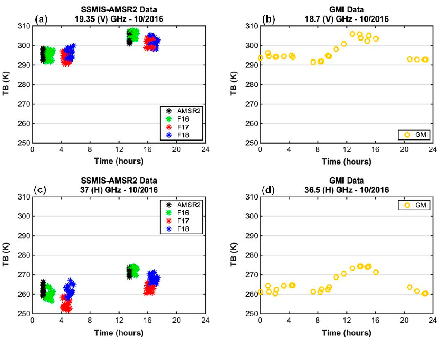
2.1. Brightness Temperature Datasets

2.1.1. GMI

The GPM Core Observatory, jointly developed by the Japan Aerospace Exploration Agency (JAXA) and National Aeronautics and Space Administration (NASA), launched on 27 February 2014. The design of this satellite is an extension of TRMM and it carries the first Ku/Ka-band dual-frequency precipitation radar (DPR) along with multi-channel GMI. It is deployed in a non-sun-synchronous orbit at a 65° inclination and a mean altitude of 407 km, giving it the effective latitudinal range of 68°N–68°S and swath width of 885 km. GMI is a conically scanning PMW radiometer onboard the GPM Core Observatory, which operates at thirteen microwave channels ranging in frequency from 10.65 to 183 ± 7 GHz. The spatial resolution of GMI on the Earth’s surface ranging from 25 km at 10 GHz to 6 km at 183 GHz. It views the Earth at an average incidence angle of 52.8° for frequencies from 10.65 to 89.0 GHz, and at 49.1° for higher frequency channels [23,24]. The GMI TB dataset used in this study is the Level 1C version 05 product, obtained from the NASA website at https://disc.gsfc.nasa.gov/ (accessed on 12 January 2021). Level 1C generates common calibrated PMW TB products for the GPM Core and constellation satellites using GMI as the reference standard [20,21]. The intercalibration process involves two major steps: (a) prescreening the sensor TB to identify and correct for calibration biases across the scan or along the orbit path, and (b) to adjust the calibrations of the constellation passive microwave radiometers to be consistent with GMI [20].

2.1.2. AMSR2

The GCOM are two series of JAXA satellites (e.g., GCOM-W and GCOM-C) designed to enable continuous global-scale observations for 10–15 years of Earth’s environmental changes. The AMSR2 sensor onboard the GCOM-W1 satellite, launched on May 17, 2012, is a conical-scanning PMW radiometer operating at six frequency channels ranging from 7 to 89 GHz [25]. It flies at about 700 km altitude with approximately 98° inclination on a sun-synchronous orbit as part of the “A-Train” satellite constellation. AMSR2 provides TB measurements over 1450 km swath width and has an incidence angle of 55°. The daily fixed acquisition times are about 1:30 and 13:30 local solar hours. Level 1C version 05 product, calibrated against GMI, used in this study was obtained from the NASA website at https://disc.gsfc.nasa.gov/ (accessed on 12 January 2021).

2.1.3. SSMIS

The series of SSMIS are satellite-borne 24-channel PMW radiometers carried onboard the suite of near-polar orbiting satellites known as US Air Force DMSP. The first of these instruments was launched on DMSP-F16 platform on 18 October 2003. In common with its predecessor SSM/I, SSMIS employs conical-scanning geometry which offers the advantage that the polarization of the measured radiances is invariant across the scan [26]. In addition, the open design permits relatively large primary reflectors and consequently affords good horizontal resolution. SSMIS is the first conical scanner to be used for temperature sounding and combines a range of temperature sounding channels (50–63 GHz), humidity sounding channels (183 GHz), as well as a range of imaging channels (19–150 GHz). SSMIS instrument is flown onboard the DMSP F-16, F-17, F-18, and F19 satellites, whereas SSMIS onboard F-19 satellite stopped providing useful data in early 2016. Fully calibrated and accurately geolocated Level 1C version 05 TB data from F16, F17, and F-18 SSMIS sensors used in this study were obtained from the NASA website at https://disc.gsfc.nasa.gov/ (accessed on 12 January 2021).

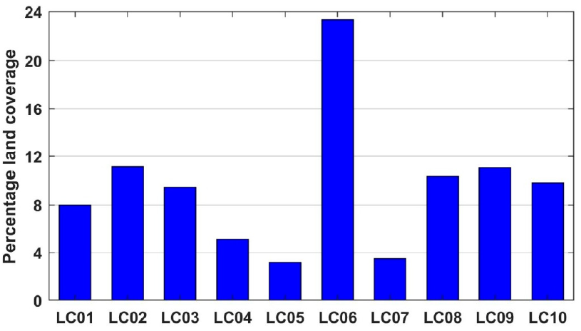
2.2. Land Cover Type Data

In this study, a global static classification of ten broad land cover types [2] derived from 32 different land cover types [27] has been used. These ten land covers include (1) tropical/sub-tropical evergreen broad-leaved forest, (2) deciduous forest, (3) evergreen broad-leaved and needle-leaved forest, (4) Deciduous woodland, (5) sclerophyllous woodland and forest, (6) wooded and non-wooded grassland, (7) tundra and mossy bog, (8) boreal and xeromorphic shrubland, (9) non-vegetated desert, and (10) ice. These ten land cover types are termed LC01 to LC10 hereafter and their percentages of global land coverage are shown in Figure 1 [28]. These static ten broad land cover types have been used in several studies.

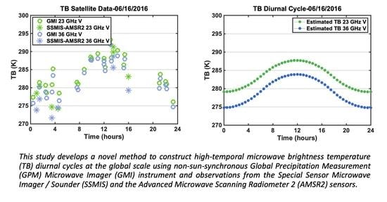
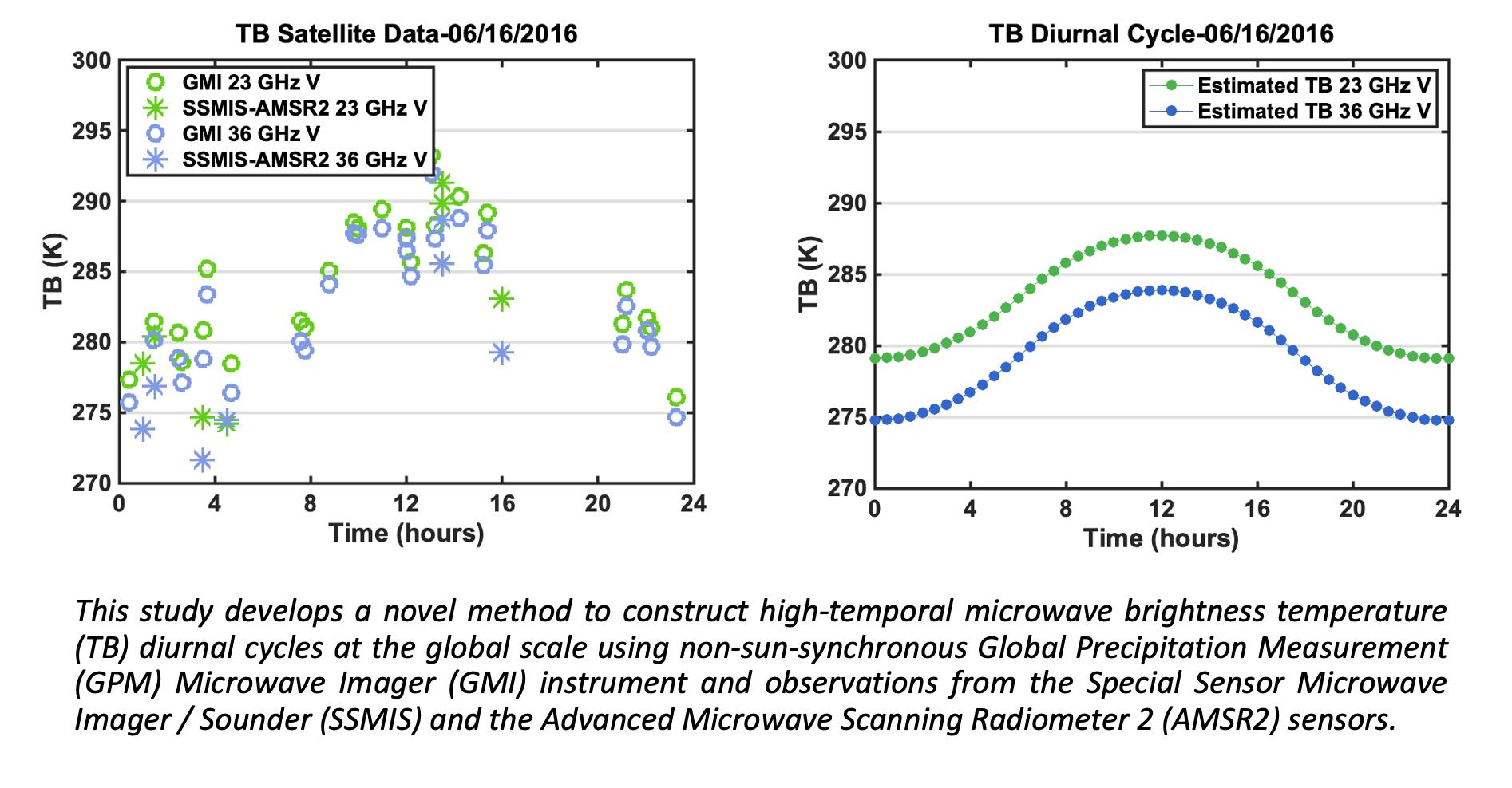
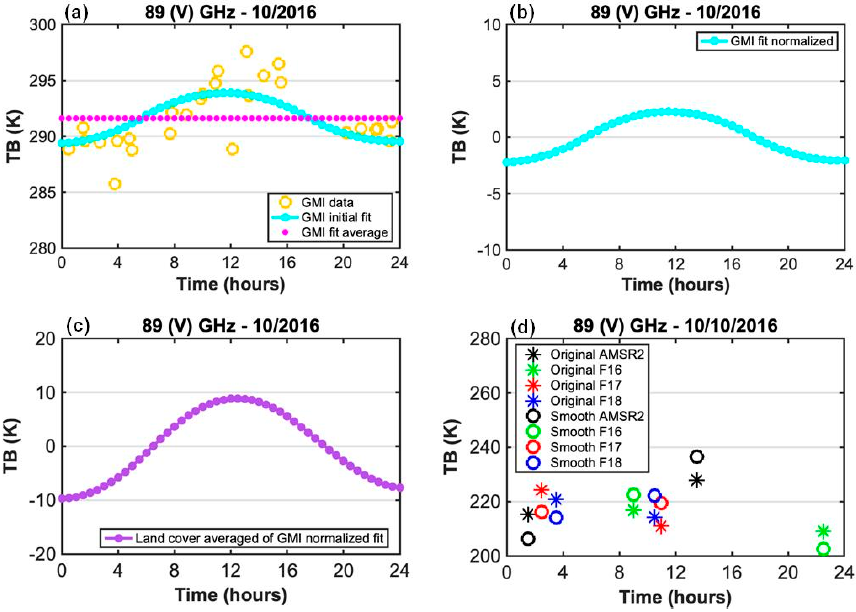
3. Computation of Diurnal Cycle of PMW TBs

In order to characterize the diurnal cycle of intercalibrated TBs, data obtained from GMI, AMSR2, and SSMIS sensors were re-projected to an equal-area grid (equivalent to 0.25° at equator) and land-only pixels were extracted for computational efficiency. The goal is to harmonize these sensors’ data in terms of channel and resolution, to construct diurnal cycle of TBs from their combination, and then to analyze TB variations across the globe. As operating frequency channels in GMI, AMSR2, and SSMIS are not essentially the same, four frequency channels around 19 GHz, 23 GHz, 37 GHz, and 89 GHz were considered to construct diurnal cycles of TBs. For brevity, only one year of TB measurements for 2016 was considered in this study and results of arbitrarily any one (or two) frequency channel(s) are shown in most of the figures.
Figure 2 shows the original records of available TBs from AMSR2, SSMIS, and GMI for October 2016 at frequency channels around 19 GHz (V) and 37 GHz (H) over a sample non-vegetated desert location (17.4°N and 28°E). TBs from all PMW sensors show a peak at afternoon as expected. Since the GMI sensor is onboard a non-sun-synchronous satellite, it provides TB measurements at several hours within a month. This makes the GMI data more suitable for diurnal analysis of TBs as well as for precipitation. In general, TBs at 19 GHz (V) are about 30K higher than TBs at 37 GHz (H) for all sensors. However, there are about 10K of TB variations at a specific time in AMSR2 and SSMIS sensors within a month.

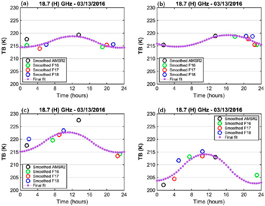
3.1. Computation of Diurnal Cycle of Land TBs between Latitude 68°S and 68°N

Taking advantage of the GMI sensor onboard a non-sun-synchronous satellite, the novel idea behind this study is to put TBs of all days of a month together to make a diurnal cycle shape for the month. Based on the previous study [7], it is reasonable to assume that general characteristics of TB diurnal variations such as amplitude do not change significantly in a month. Hence, half-hourly TB is constructed from a whole month with the GMI product by applying a mathematical method in the initial step. The mathematical fit utilized here is the least-squares approximation by cubic splines. Spline functions and, more generally, piecewise polynomial functions are some of the most successful approximating functions for such applications. The spline interpolation method has been successfully applied to study the diurnal variations of infrared land surface temperature (LST) and passive microwave TBs [6,28,29,30]. They combine ease of computational handling with great flexibility; therefore, they are particularly appropriate for the approximation of experimental data or design curve measurements.
In the next step, differences between daily SSMIS/AMSR2 measurements and constructed monthly GMI data on corresponding time points (∆i) were calculated for each day and for all the pixels between latitude 68°S and 68°N. For instance, for each of the timing points with available observation data, ∆i would be the difference between the interpolated GMI fit and the corresponding AMSR2, SSMIS F16, SSMIS F17, and SSMIS F18 data. This difference is given by:
Δi = TBAMSR2/SSMISTBGMI
The schematic estimation process of ∆i is depicted in Figure 3a for a sample location with non-vegetated land cover for 15 January 2016. The original GMI, AMSR2, SSMIS F16, SSMIS F17, and SSMIS F18 observations and the interpolated GMI fit for 18.7 GHz (V) are also shown in the figure.
Finally, the diurnal cycle (TBfinal) is computed by taking the average of (∆i) s and then adding this value to the GMI initial fit, as follows:
  =   ( i = 1 8 i / n )
T B f i n a l = T B G M I +
Figure 3b demonstrates the corrected TB diurnal cycle by adding ∆ to the GMI initial fit. Figure 4 illustrates the constructed TB diurnal variations at 37 GHz (V) at four different dates and four sample locations (two in Northern and two in Southern Hemisphere) having distinct vegetation types. The original TBs from each sensor are also shown in the figure.
Monthly mean differences between GMI and SSMIS/AMSR2 data for each land cover type in 2016 for channel 23 GHz (V) are shown in Table 1. The differences are generally between 1K and 3K. Only during a few months does the tundra and mossy bog land cover type (LC07) show higher values (above 10K) than the other land vegetation types. This particular land cover is only available in the Northern Hemisphere near Arctic regions. In recent years, it has gone under enormous changes due to a large number of disturbances and climate forcing such as wildfires. Considering 31-year satellite imagery, extensive shifts in the distribution of plant functional types and ecosystem productivity have been observed in response to the climate change [31]. It is worthwhile to mention that the spatial resolution of existing land cover datasets is not fine enough; small-scale land cover changes in this vegetation cover have been poorly characterized.

3.2. Computation of Diurnal Cycle of Land TBs above Latitude 68°N and below Latitude 68°S

Since there are no GMI data available for latitudes over 68°N and below 68°S, a new estimation method has to be developed for constructing TB diurnal cycles in those areas. Herein, the GMI data have been used as a point of reference to smooth the SSMIS and AMSR2 data in polar regions. For this reason, the TB diurnal cycle from GMI fit was normalized by taking the daily average away for each pixel. Then, for each of the ten land cover types, the average of the normalized graph was calculated. In the next step, the aforementioned normalized graph was applied to the SSMIS/AMSR2 data in the regions not covered by the GMI to obtain the smoothed data. Figure 5 represents the smoothing method step by step in details.
Finally, the spline fit was applied to the smoothed AMSR2, SSMIS F16, SSMIS F17, and SSMIS F18 data to estimate the half-hourly TB diurnal cycle in polar regions. Final TB diurnal interpolations at 18.7 GHz (H) for four sample locations (three in Northern and one in Southern Hemisphere) having distinct land cover types are shown in Figure 6. As expected, the magnitude and timing of maximum TBs are notably different for distinct land cover types.

4. Results and Discussion

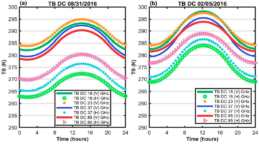
4.1. Assessment of the Global Land Diurnal Cycle of PMW TBs

In order to assess the accuracy of the proposed method qualitatively, TB diurnal cycles at four PMW bands have been compared for different seasons and for two distinct land covers in Figure 7. It is preliminarily observed that the vertical polarization shows higher values in comparison to horizontal polarization. Additionally, as the channel frequency increases, the difference between vertical and horizontal TB values decreases. However, the differences between both vertical and horizontal polarizations at any frequency channel is larger for boreal and xeromorphic shrubland land cover than that for wooded and non-wooded grassland land cover. The magnitude of diurnal cycle of TB at 23 GHz (V) is the largest as compared to other frequency channels for boreal and xeromorphic shrubland land cover, while it is comparable to 19GHz (V) for wooded and non-wooded grassland land cover. Moreover, the peak in the diurnal cycle is about two hours earlier over wooded and non-wooded grassland land cover than that over boreal and xeromorphic shrubland land cover. However, the magnitude of peak diurnal TBs is always higher for wooded and non-wooded grassland land cover than boreal and xeromorphic shrubland land cover. It is worthwhile to note that these results are in good agreement with previous studies by Norouzi et al. [6,7] and Aljassar et al. [32]. Furthermore, the shape and peak of the obtained TB diurnal cycle is almost similar to the LST diurnal cycle as proposed by Sharifnezhadazizi et al. [28].

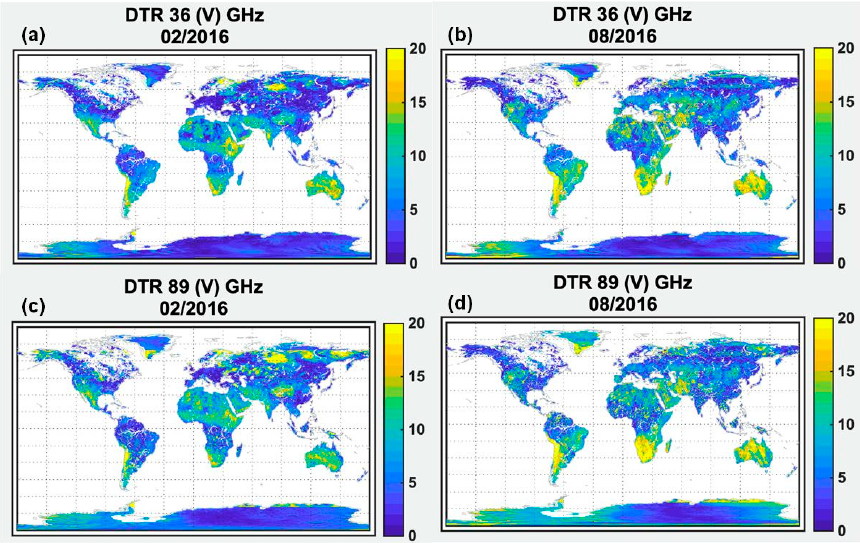
4.2. Spatial Distributions of Global Land Diurnal Brightness Temperature Range

The diurnal cycle of TBs enables the computation of magnitudes and time of occurrence of daily maximum and minimum TBs. The difference in daily maximum and minimum TB estimates is termed as diurnal brightness temperature range (DTR). Figure 8 illustrates the global mean monthly DTR derived from the estimated half-hourly TBs for two PMW bands of 37 GHz and 89 GHz at vertical polarization and for two contrasting months of February and August of 2016.
In general, DTR shows large spatial variation during both months. In the Northern Hemisphere, the largest magnitudes of DTR (>15 K) are evident in Mexico, the Sahara in North Africa, Western Asia, and parts of Siberia in Russia. In the Southern Hemisphere, the Kalahari Desert in the Southern Africa, Madagascar, shrublands of the Andes Mountain chain in South America, and Australian deserts are regions with the most noticeable DTR. Right on the equator, the horn of Africa is another region with high DTR values. To recap, DTR is consistently large over the three land cover types: wooded and non-wooded grassland, boreal and xeromorphic shrubland, and tundra and mossy bog. Since in the fall and spring seasons, the emissivity values of forest canopy, frozen ground, and wet snow were relatively close to each other, the mean TBs show similar variations [33]. Lower DTR (<5 K) can be found in all sorts of forests: tropical rainforests, deciduous forests, and even evergreen broad-leaved and needle-leaved forests. Generally, DTR characteristics exhibit noticeable differences with both latitude and land cover. It is most likely that the vegetation type has a systematic effect on solar reflection and surface emissions [34,35].
The mean monthly DTR averaged over different land cover types for both hemispheres was shown in Figure 9. These results correspond to two contrasting seasons and four different PMW bands at vertical polarization. In general, the calculated values for the Southern Hemisphere display an orderly relation among DTR, land cover type and season. It is evident that the DTR is higher during July (e.g., Southern Hemispheric winter) than in January (e.g., Southern Hemispheric summer) for all land cover types. In the Northern Hemisphere, each PMW band shows slightly distinct behavior. The only land cover which presents a consistent behavior is the non-vegetated desert where DTR is higher during July in comparison to January. In most of the desert regions, as the frequency increases and the penetration depth becomes smaller, the radiometric measurements display larger diurnal variations. Moreover, in arid regions, the effect of the atmosphere is more considerable at higher frequencies [36,37,38]. The rest of the land cover types with more vegetation and higher moisture content generally show a rather lower DTR. This is in line with previous studies [6,7] that reported the effect moisture and vegetation on the TB DTR. In terms of seasonal comparison, higher DTR amplitudes are evident during January (e.g., Northern Hemispheric winter) than in July (e.g., Northern Hemispheric summer) at 89 GHz expect for desert regions. As the microwave frequency becomes lower to 89 GHz (e.g., 37 GHz, 23 GHz, and 19 GHz), the behavior of seasonal variations in DTR varies for different land cover types with less consistency.
Figure 10 illustrates a comparison between monthly DTR from the initial GMI diurnal cycle and from the final half-hourly TB product for June 2016 at 23 GHz with vertical polarization. It can be seen that the value of GMI DTR in each pixel is almost the same as the DTR derived by the final TB product over the GPM coverage region (e.g., between 68°S and 68°N). The reason behind this agreement is that the GMI diurnal cycle has been herein moved with respect to SSMIS/AMSR2 daily data with preserving the shape and amplitude of the diurnal cycle. The only improvement from the final half-hourly TBs is that one can obtain DTR maps for the polar regions as well while maintaining consistency.

5. Summary and Conclusions

In this paper, a procedure for retrieving and estimating high temporal resolution TB diurnal cycles using multi-satellite PMW observations was introduced. A one-year data record of intercalibrated land TBs from the GMI, AMSR2, and three SSMIS sensors from nearly common frequencies with both horizontal and vertical polarizations was utilized for 2016 in this study. A spline fit was primarily applied to monthly GMI data between 68°N and 68°S latitudes and then the estimated half-hourly TB diurnal cycle was enhanced by AMSR2 and SSMIS daily values in order to obtain a more precise diurnal cycle. For the areas above 68°N and below 68°S, a novel method was introduced to smooth the SSMIS and AMSR2 data based on GMI normalized diurnal cycle on each of the ten land cover types. This is the first time that we are able to construct a TB diurnal cycle with the existence of time varying GMI TB observations. Evaluation of the constructed diurnal cycle of TBs was performed by qualitative comparison at different frequencies and polarizations for distinct land cover types. It was found that the present method showed promising results in capturing the diurnal variations of PMW TBs for different land cover types. Furthermore, the interpolated half-hourly TB data were used to calculate the DTR parameters. An almost consistent variability was found among the different land cover types. A larger DTR of more than 15 K was observed over the grassland, shrubland, and tundra, whereas a smaller DTR of less than 5 K was evident over the forests. However, seasonal variations in DTR for different land cover types showed a more consistent result over the Southern Hemisphere than over the Northern Hemisphere. Analysis of global DTR was also performed to find correlation among DTR, latitude, season, land cover, and PMW frequency channels.
The half-hourly PMW TBs derived in this study could be further used to retrieve high temporal resolution land surface emissivity diurnal cycle in order to characterize surface FT conditions. This would enhance temporal detection of FT which is more helpful during the transition times when multiple FT changes may occur within a day. As accurate detection of FT changes, especially in the high-latitude regions, is crucial for several applications such as for the terrestrial water cycle, net primary productivity, methane cycle, and surface energy budget, the proposed method would enable the detection of finer temporal resolution FT states. Nevertheless, there are uncertainties in the present interpolation method due to factors such as footprint, frequency, and incidence angle differences among the sensors. In addition, there are differences in local solar time for the same pixel on different revisit days of the radiometers due to their intrinsic scanning characteristics. These characteristics produce discrepancies to some extent that need further investigation. This study can further benefit from comparisons with a global network of ground-based observations to obtain a more comprehensive validation.

Author Contributions

Conceptualization, Z.S. and H.N.; formal analysis, Z.S. and H.N.; writing—original draft preparation, Z.S., and S.P.; writing—review and editing, S.P., H.N., R.B. and R.K.; supervision, H.N. and R.K. All authors have read and agreed to the published version of the manuscript.

Funding

This research was supported by the National Oceanic and Atmospheric Administration—Cooperative Science Center for Earth System Sciences and Remote Sensing Technologies (NOAA–CESSRST) under the Cooperative Agreement Grant NA16SEC4810008, by the NASA under Grant NNH15ZDA001N, and by the Center for Remote Sensing and Earth System Sciences at the New York City College of Technology.

Acknowledgments

The authors thank the anonymous reviewers and the editor for their constructive comments and suggestions. The intercalibrated passive microwave brightness temperature datasets obtained from the NASA’s Goddard Space Flight Center are thankfully acknowledged.

Conflicts of Interest

The authors declare no conflict of interest. The funders had no role in the design of the study; in the collection, analyses, or interpretation of data; in the writing of the manuscript, or in the decision to publish the results.

References

  1. Liu, G.; Curry, J.A. Retrieval of precipitation from satellite microwave measurement using both emission and scattering. J. Geophys. Res. Atmos. 1992, 97, 9959–9974. [Google Scholar] [CrossRef]
  2. Prigent, C.; Rossow, W.B.; Matthews, E. Global maps of microwave land surface emissivities: Potential for land surface characterization. Radio Sci. 1998, 33, 745–751. [Google Scholar] [CrossRef]
  3. Njoku, E.G.; Jackson, T.J.; Lakshmi, V.; Chan, T.K.; Nghiem, S.V. Soil moisture retrieval from AMSR-E. IEEE Trans. Geosci. Remote Sens. 2003, 41, 215–229. [Google Scholar] [CrossRef]
  4. Karbou, F.; Gérard, É.; Rabier, F. Microwave land emissivity and skin temperature for AMSU-A and -B assimilation over land. Q. J. R. Meteorol. Soc. 2006, 132, 2333–2355. [Google Scholar] [CrossRef] [Green Version]
  5. Min, Q.L.; Lin, B.; Li, R. Remote sensing vegetation hydrological states using passive microwave measurements. IEEE J. Sel. Top. Appl. Earth Obs. Remote Sens. 2010, 3, 124–131. [Google Scholar] [CrossRef]
  6. Norouzi, H.; Rossow, W.; Temimi, M.; Prigent, C.; Azarderakhsh, M.; Boukabara, S.; Khanbilvardi, R. Using microwave brightness temperature diurnal cycle to improve emissivity retrievals over land. Remote Sens. Environ. 2012, 123, 470–482. [Google Scholar] [CrossRef] [Green Version]
  7. Norouzi, H.; Temimi, M.; AghaKouchak, A.; Azarderakhsh, M.; Khanbilvardi, R.; Shields, G.; Tesfagiorgis, K. Inferring land surface parameters from the diurnal variability of microwave and infrared temperatures. Phys. Chem. Earth Parts 2015, 83, 28–35. [Google Scholar] [CrossRef]
  8. Li, Z.L.; Tang, B.H.; Wu, H.; Ren, H.; Yan, G.; Wan, Z.; Trigo, I.F.; Sobrino, J.A. Satellite-derived land surface temperature: Current status and perspectives. Remote Sens. Environ. 2013, 131, 14–37. [Google Scholar] [CrossRef] [Green Version]
  9. Zhou, F.-C.; Song, X.; Leng, P.; Wu, H.; Tang, B.-H. An algorithm for retrieving precipitable water vapor over land based on passive microwave satellite data. Adv. Meteorol. 2016, 2016. [Google Scholar] [CrossRef] [Green Version]
  10. Prakash, S.; Norouzi, H.; Azarderakhsh, M.; Blake, R.; Prigent, C.; Khanbilvardi, R. Estimation of consistent global microwave land surface emissivity from AMSR-E and AMSR2 observations. J. Appl. Meteorol. Climatol. 2018, 57, 907–919. [Google Scholar] [CrossRef]
  11. You, Y.; Munchak, S.J.; Ferraro, R.; Mohr, K.; Peters-Lidard, C.; Prigent, C.; Ringerud, S.; Rudlosky, S.; Wang, H.; Norouzi, H.; et al. Raindrop signature from microwave radiometer over deserts. Geophys. Res. Lett. 2020, 47, e2020GL088656. [Google Scholar] [CrossRef]
  12. Zhang, T.; Armstrong, R.L. Soil freeze/thaw cycles over snow-free land detected by passive microwave remote sensing. Geophys. Res. Lett. 2001, 28, 763–766. [Google Scholar] [CrossRef]
  13. Kim, Y.; Kimball, J.S.; McDonald, K.C.; Glassy, J. Developing a global data record of daily landscape freeze/thaw status using satellite passive microwave remote sensing. IEEE Trans. Geosci. Remote Sens. 2011, 49, 949–960. [Google Scholar] [CrossRef]
  14. Podest, E.; McDonald, K.C.; Kimball, J.S. Multisensor microwave sensitivity to freeze/thaw dynamics across a complex boreal landscape. IEEE Trans. Geosci. Remote Sens. 2014, 52, 6818–6828. [Google Scholar] [CrossRef]
  15. Derksen, C.; Xu, X.; Dunbar, R.S.; Colliander, A.; Kim, Y.; Kimball, J.S.; Black, T.A.; Euskirchen, E.; Langlois, A.; Loranty, M.M.; et al. Retrieving landscape freeze/thaw state from Soil Moisture Active Passive (SMAP) radar and radiometer measurements. Remote Sens. Environ. 2017, 194, 48–62. [Google Scholar] [CrossRef]
  16. Prakash, S.; Norouzi, H.; Azarderakhsh, M.; Blake, R.; Khanbilvardi, R. Potential of satellite-based land emissivity estimates for the detection of high-latitude freeze and thaw states. Geophys. Res. Lett. 2017, 44, 2336–2342. [Google Scholar] [CrossRef] [Green Version]
  17. Zhao, T.; Shi, J.; Hu, T.; Zhao, L.; Zou, D.; Wang, T.; Ji, D.; Li, R.; Wang, P. Estimation of high-resolution near-surface freeze/thaw state by the integration of microwave and thermal infrared remote sensing data on the Tibetan Plateau. Earth Space Sci. 2017, 4, 472–484. [Google Scholar] [CrossRef]
  18. Bartsch, A.; Kidd, R.A.; Wagner, W.; Bartalis, Z. Temporal and spatial variability of the beginning and end of daily spring freeze/thaw cycles derived from scatterometer data. Remote Sens. Environ. 2007, 106, 360–374. [Google Scholar] [CrossRef]
  19. Wilheit, T.; Berg, W.; Ebrahimi, H.; Kroodsma, R.; McKague, D.; Payne, V.; Wang, J. Intercalibrating the GPM Constellation Using the GPM Microwave Imager (GMI). In Proceedings of the 2015 IEEE International Geoscience and Remote Sensing Symposium (IGARSS), Milan, Italy, 26–31 July 2005; pp. 5162–5165. [Google Scholar] [CrossRef]
  20. Berg, W.; Bilanow, S.; Chen, R.; Datta, S.; Draper, D.; Ebrahimi, H.; Farrar, S.; Jones, W.L.; Kroodsma, R.; McKague, D.; et al. Intercalibration of the GPM microwave radiometer constellation. J. Atmos. Ocean. Technol. 2016, 33, 2639–2654. [Google Scholar] [CrossRef]
  21. Berg, W.; Kroodsma, R.; Kummerow, C.D.; McKague, D.S. Fundamental climate data records of microwave brightness temperatures. Remote Sens. 2018, 10, 1306. [Google Scholar] [CrossRef] [Green Version]
  22. Holmes, T.R.H.; Crow, W.T.; Yilmaz, M.T.; Jackson, T.J.; Basara, J.B. Enhancing model-based land surface temperature estimates using multiplatform microwave observations. J. Geophys. Res. Atmos. 2013, 118, 577–591. [Google Scholar] [CrossRef]
  23. Draper, D.W.; Newell, D.A.; Wentz, F.J.; Krimchansky, S.; Skofronick-Jackson, G.M. The Global Precipitation Measurement (GPM) Microwave Imager (GMI): Instrument overview and early on-orbit performance. IEEE J. Sel. Top. Appl. Earth Obs. Remote Sens. 2015, 8, 3452–3462. [Google Scholar] [CrossRef]
  24. Duncan, D.I.; Kummerow, C.D. A 1DVAR retrieval applied to GMI: Algorithm description, validation, and sensitivities. J. Geophys. Res. Atmos. 2016, 121, 7415–7429. [Google Scholar] [CrossRef] [Green Version]
  25. Okuyama, A.; Imaoka, K. Intercalibration of Advanced Microwave Scanning Radiometer-2 (AMSR2) brightness temperature. IEEE Trans. Geosci. Remote Sens. 2015, 53, 4568–4577. [Google Scholar] [CrossRef]
  26. Kunkee, D.B.; Poe, G.A.; Boucher, D.J.; Swadley, S.D.; Hong, Y.; Wessel, J.E.; Uliana, E.A. Design and evaluation of the first Special Sensor Microwave Imager/Sounder. IEEE Trans. Geosci. Remote Sens. 2008, 46, 863–883. [Google Scholar] [CrossRef]
  27. Matthews, E. Global vegetation and land use: New high-resolution data bases for climate studies. J. Clim. Appl. Meteorol. 1983, 22, 474–487. [Google Scholar] [CrossRef] [Green Version]
  28. Sharifnezhadazizi, Z.; Norouzi, H.; Prakash, S.; Beale, C.; Khanbilvardi, R. A global analysis of land surface temperature diurnal cycle using MODIS observations. J. Appl. Meteorol. Climatol. 2019, 58, 1279–1291. [Google Scholar] [CrossRef]
  29. Aires, F.; Prigent, C.; Rossow, W.B. Temporal interpolation of global surface skin temperature diurnal cycle over land under clear and cloudy conditions. J. Geophys. Res. Atmos. 2004, 109. [Google Scholar] [CrossRef]
  30. Beale, C.; Norouzi, H.; Sharifnezhadazizi, Z.; Bah, A.R.; Yu, P.; Yu, Y.; Blake, R.; Vaculik, A.; Gonzalez-Cruz, J. Comparison of diurnal variation of land surface temperature from GOES-16 ABI and MODIS instruments. IEEE Geosci. Remote Sens. Lett. 2019, 17, 572–576. [Google Scholar] [CrossRef]
  31. Wang, J.A.; Sulla-Menashe, D.; Woodcock, C.E.; Sonnentag, O.; Keeling, R.F.; Friedl, M.A. Extensive land cover change across Arctic—Boreal Northwestern North America from disturbance and climate forcing. Glob. Chang. Biol. 2020, 26, 807–822. [Google Scholar] [CrossRef]
  32. AlJassar, H.K.; Temimi, M.; Entekhabi, D.; Petrov, P.; AlSarraf, H.; Kokkalis, P.; Roshni, N. Forward simulation of multi-frequency microwave brightness temperature over desert soils in Kuwait and comparison with satellite observations. Remote Sens. 2019, 11, 1647. [Google Scholar] [CrossRef] [Green Version]
  33. Kurvonen, L.; Hallikainen, M. Influence of land-cover category on brightness temperature of snow. IEEE Trans. Geosci. Remote Sens. 1997, 35, 367–377. [Google Scholar] [CrossRef]
  34. Joseph, A.T.; van der Velde, R.; O’Neill, P.E.; Choudhury, B.J.; Lang, R.H.; Kim, E.J.; Gish, T. L band brightness temperature observations over a corn canopy during the entire growth cycle. Sensors 2010, 10, 6980–7001. [Google Scholar] [CrossRef] [PubMed] [Green Version]
  35. Sahana, M.; Ahmed, R.; Sajjad, H. Analyzing land surface temperature distribution in response to land use/land cover change using split window algorithm and spectral radiance model in Sundarban Biosphere Reserve, India. Model. Earth Syst. Environ. 2016, 2, 81. [Google Scholar] [CrossRef] [Green Version]
  36. Grody, N.C.; Weng, F. Microwave emission and scattering from deserts: Theory compared with satellite measurements. IEEE Trans. Geosci. Remote Sens. 2008, 46, 361–375. [Google Scholar] [CrossRef]
  37. Prigent, C.; Rossow, W.B.; Matthews, E.; Marticorena, B. Microwave radiometric signatures of different surface types in deserts. J. Geophys. Res. Atmos. 1999, 104, 12147–12158. [Google Scholar] [CrossRef] [Green Version]
  38. Norouzi, H.; Temimi, M.; Prigent, C.; Turk, J.; Khanbilvardi, R.; Tian, Y.; Furuzawa, F.; Masunaga, H. Assessment of the consistency among global microwave land surface emissivity products. Atmos. Meas. Tech. 2015, 8, 1197–1205. [Google Scholar] [CrossRef] [Green Version]
Figure 1. Percentage global land coverage of ten land cover types: namely, tropical/sub-tropical evergreen broad-leaved forest (LC01), deciduous forest (LC02), evergreen broad-leaved and needle-leaved forest (LC03), deciduous woodland (LC04), sclerophyllous woodland and forest (LC05), wooded and non-wooded grassland (LC06), tundra and mossy bog (LC07), boreal and xeromorphic shrubland (LC08), non-vegetated desert (LC09), and ice (LC10).
Remotesensing 13 00817 g001
Figure 2. Satellite-borne passive microwave brightness temperature (PMW TB) observations at a sample location (17.4°N and 28°E) with non-vegetated desert land cover for October 2016 using (a) SSMIS F16, F17, F18, and AMSR2 at 19.35 GHz vertical polarization; (b) GMI at 18.7 GHz vertical polarization; (c) SSMIS F16, F17, F18, and AMSR2 at 37 GHz horizontal polarization; (d) GMI at 36.5 GHz horizontal polarization. Time in each subplot is in local solar hours.
Remotesensing 13 00817 g002
Figure 3. Schematic to compute diurnal cycle of PMW TBs for pixels between 68°S and 68°N, at a sample location (25.1°S and 138.6°E) with non-vegetated desert land cover for 15 January 2016 at 18.7 GHz vertical polarization (a) based on monthly GMI data, and (b) corrected by AMSR2 and SSMIS daily data. Time in each subplot is in local solar hours.
Remotesensing 13 00817 g003
Figure 4. Diurnal variations of interpolated TB at 37 GHz vertical polarization for (a) 17.9°S and 36.4°E with wooded and non-wooded grassland land cover for June 16, 2016; (b) 8.1°S and 26.6°E with deciduous woodland land cover for 1 October 2016; (c) 17.4°N and 28.1°E with non-vegetated desert land cover for 9 February 2016; and (d) 27.4°N and 115.1°E with evergreen broad-leaved and needle-leaved forest land cover for 27 December 2016. Time in each subplot is in local solar hours.
Remotesensing 13 00817 g004
Figure 5. Steps for SSMIS/AMSR2 data smoothing for regions above latitude 68°N and below latitude 68°S at 89 GHz vertical polarization. (a) Initial GPM Microwave Imager (GMI) fit and its average for a sample location at 13.9°N and 14°W with deciduous woodland land cover for October 2016; (b) normalized GMI fit by taking away the average from the initial fit for the same location and month; (c) the average of all the GMI normalized plots for pixels with the same land cover and month; (d) smoothing of the original SSMIS/AMSR2 data for a sample location at 71.2°N and 103°E with the same land cover and month by applying the land cover-averaged normalized plot on the corresponding time for 10 October 2016. Time in each subplot is in local solar hours.
Remotesensing 13 00817 g005
Figure 6. Diurnal variations of interpolated TB out of smoothed SSMIS F16, F17, F18, and AMSR2 for sample locations with different land covers for 13 March 2016 at 18.7 GHz horizontal polarization for (a) 71.5°S and 12.9°E with ice land cover, (b) 73.7°N and 122°W with tundra and mossy bog land cover, (c) 71°N and 114°E with deciduous woodland land cover, and (d) 77°N and 106.4°E with non-vegetated desert land cover. Time in each subplot is in local solar hours.
Remotesensing 13 00817 g006
Figure 7. Comparison of constructed TB diurnal cycle for different PMW channels in two contrasting seasons at (a) 45.9°N and 103°W with boreal and xeromorphic shrubland land cover for 31 August 2016; and (b) 3.6°N and 142.7°W with wooded and non-wooded grassland land cover for 5 February 2016. Time in each subplot is in local hours.
Remotesensing 13 00817 g007
Figure 8. Spatial distributions of monthly diurnal brightness temperature range (DTR) (K) at (a,b) 37 GHz vertical polarization, and (c,d) 89 GHz vertical polarization for two contrasting seasons of (a,c) February 2016 and (b,d) August 2016.
Remotesensing 13 00817 g008
Figure 9. Mean monthly DTR averaged over different land cover types for two contrasting seasons of January 2016 and July 2016 for the (a,c,e,g) Northern Hemisphere, and the (b,d,f,h) Southern Hemisphere at (a,b) 19 GHz vertical polarization, (c,d) 23 GHz vertical polarization, (e,f) 37 GHz vertical polarization, and (g,h) 89 GHz vertical polarization.
Remotesensing 13 00817 g009
Figure 10. Global DTR (K) map (a) from initial GMI TB values, and (b) expanded to the polar region from GMI final interpolated TB values for June 2016 at 23 GHz vertical polarization.
Remotesensing 13 00817 g010
Table 1. Mean monthly differences between GMI and SSMIS/AMSR2 data for each land cover types at 23 GHz vertical polarization.
Jan.Feb.Mar.Apr.MayJun.Jul.Aug.Sep.Oct.Nov.Dec.
LC011.560.810.931.171.080.721.071.241.340.601.211.10
LC022.073.112.882.153.881.472.173.032.162.312.121.66
LC032.273.262.431.723.671.351.963.521.891.942.121.48
LC042.342.233.002.223.281.621.663.742.921.243.132.07
LC052.181.942.391.933.441.382.063.472.791.302.132.09
LC062.793.052.552.323.891.862.643.773.052.182.342.50
LC073.206.415.8915.766.082.833.494.9316.942.313.1715.20
LC082.972.702.512.743.941.932.613.693.712.092.592.93
LC092.994.152.331.964.371.473.123.883.743.102.512.49
LC102.082.791.883.222.242.922.855.113.243.603.833.17
Publisher’s Note: MDPI stays neutral with regard to jurisdictional claims in published maps and institutional affiliations.

