
Analysis of Atmospheric and Ionospheric Variations Due to Impacts of Super Typhoon Mangkhut (1822) in the Northwest Pacific Ocean

 ,
, 
 ,
,  , ,
, ,  ,
,
Abstract
:
1. Introduction
2. Data Sources and Analysis Methods
2.1. Space Environment and Super Typhoon Mangkhut Data
2.2. Atmospheric Parameters
2.3. Calculation Process of STEC, VTEC, and RIMs
2.4. Methods For Detecting VTEC Disturbances.
3. Results and Discussion
3.1. Geomagnetic Field and Solar-Terrestrial Environment
3.2. Ionospheric Variations During Super Typhoon Mangkhut
3.3. Atmospheric Observations During Super Typhoon Mangkhut
4. Conclusions
Author Contributions
Funding
Institutional Review Board Statement
Informed Consent Statement
Data Availability Statement
Acknowledgments
Conflicts of Interest
References
- Sojka, J.J.; Raitt, W.J.; Schunk, R.W. Theoretical predictions for ion composition in the high-latitude winter F-region for solar minimum and low magnetic activity. J. Geophys. Res. Space Phys. 1981, 86, 609–621. [Google Scholar] [CrossRef]
- Hargreaves, J.K. The Solar-Terrestrial Environment; Cambridge University Press: Cambridge, UK, 1992. [Google Scholar]
- Schunk, R.W.; Sojka, J.J. Global ionosphere-polar wind system during changing magnetic activity. J. Geophys. Res. Space Phys. 1997, 102, 11625–11651. [Google Scholar] [CrossRef]
- Breus, T.K.; Krymskii, A.M.; Crider, D.H.; Ness, N.F.; Hinson, D.; Barashyan, K.K. Effect of the solar radiation in the topside atmosphere/ionosphere of Mars: Mars Global Surveyor observations. J. Geophys. Res. Space Phys. 2004, 109. [Google Scholar] [CrossRef]
- Chane-ming, F.; Roff, G.; Robert, L.; Leveau, J. Gravity wave characteristics over Tromelin Island during the passage of cyclone Hudah. Geophys. Res. Lett. 2002, 29, 18-1–18-4. [Google Scholar] [CrossRef]
- Guha, A.; Paul, B.; Chakraborty, M.; De, B.K. Tropical cyclone effects on the equatorial ionosphere: First result from the Indian sector. J. Geophys. Res. Space Phys. 2016, 121, 5764–5777. [Google Scholar] [CrossRef] [Green Version]
- Kim, S.; Chun, H.; Baik, J.J. A numerical study of gravity waves induced by convection associated with Typhoon Rusa. Geophys. Res. Lett. 2005, 32, L24816. [Google Scholar] [CrossRef]
- Cowling, D.H.; Webb, H.D.; Yeh, K.C. Group rays of internal gravity waves in a wind-stratified atmosphere. J. Geophys. Res. 1971, 76, 213–220. [Google Scholar] [CrossRef]
- Sorokin, V.M.; Chmyrev, V.M.; Yaschenko, A.K. Electrodynamic model of the lower atmosphere and the ionosphere coupling. J. Atmos. Sol.-Terr. Phys. 2001, 63, 1681–1691. [Google Scholar] [CrossRef]
- Afraimovich, E.L.; Voeykov, S.V.; Ishin, A.B.; Perevalova, N.P.; Ruzhin, Y.Y. Variations in the total electron content during the powerful typhoon of August 5–11, 2006, near the southeastern coast of China. Geomagn. Aeron. 2008, 48, 674–679. [Google Scholar] [CrossRef]
- Hines, C.O. Internal atmospheric gravity waves at ionospheric heights. Can. J. Phys. 1960, 38, 1441–1481. [Google Scholar] [CrossRef]
- Ilin, N.V.; Slyunyaev, N.N.; Mareev, E.A. Toward a Realistic Representation of Global Electric Circuit Generators in Models of Atmospheric Dynamics. J. Geophys. Res. Atmos. 2020, 125. [Google Scholar] [CrossRef]
- Polyakova, A.S.; Perevalova, N.P. Investigation into impact of tropical cyclones on the ionosphere using GPS sounding and NCEP/NCAR Reanalysis data. Adv. Space Res. 2011, 48, 1196–1210. [Google Scholar] [CrossRef]
- Polyakova, A.S.; Perevalova, N.P. Comparative analysis of TEC disturbances over tropical cyclone zones in the North-West Pacific Ocean. Adv. Space Res. 2013, 52, 1416–1426. [Google Scholar] [CrossRef]
- Emanuel, K. Tropical cyclones. Annu. Rev. Earth Planet. Sci. 2003, 31, 75–104. [Google Scholar] [CrossRef]
- Pielke, R.A., Jr.; Pielke, R.A., Sr. Hurricanes: Their Nature and Impacts on Society; John Wiley and Sons: Chichester, NY, USA, 1997. [Google Scholar]
- Pokrovskaya, I.V.; Sharkov, E.A. Tropical Cyclones and Tropical Disturbances of the World Ocean: Chronology and Evolution, version 3.1 (1983–2005); Poligraph Services: Moscow, Russia, 2006. [Google Scholar]
- Bauer, S.J. Correlations between tropospheric and ionospheric parameters. Geofis. Pura E Appl. 1958, 40, 235–240. [Google Scholar] [CrossRef]
- Zhao, Q.; Yao, Y.; Yao, W. GPS-based PWV for precipitation forecasting and its application to a typhoon event. J. Atmos. Sol.-Terr. Phys. 2018, 167, 124–133. [Google Scholar] [CrossRef]
- Zhao, Y.; Mao, T.; Wang, J.S.; Chen, Z. The 2D features of tropical cyclone Usagi’s effects on the ionospheric total electron content. Adv. Space Res. 2018, 62, 760–764. [Google Scholar] [CrossRef]
- Hocke, K.; Schlegel, K. A review of atmospheric gravity waves and travelling ionospheric disturbances: 1982–1995. Ann. Geophys. 1996, 14, 917. [Google Scholar]
- Kazimirovsky, E.; Herraiz, M.; De la Morena, B.A. Effects on the ionosphere due to phenomena occurring below it. Surv. Geophys. 2003, 24, 139–184. [Google Scholar] [CrossRef]
- Laštovička, J. Forcing of the ionosphere by waves from below. J. Atmos. Sol.-Terr. Phys. 2006, 68, 479–497. [Google Scholar] [CrossRef]
- Isaev, N.V.; Sorokin, V.M.; Chmyrev, V.M.; Serebryakova, O.N.; Yashchenko, A.K. Disturbance of the Electric Field in the Ionosphere by Sea Storms and Typhoons. Cosm. Res. 2002, 40, 547–553. [Google Scholar] [CrossRef]
- Isaev, N.V.; Kostin, V.M.; Belyaev, G.G.; Ovcharenko, O.Y.; Trushkina, E.P. Disturbances of the topside ionosphere caused by typhoons. Geomagn. Aeron. 2010, 50, 243–255. [Google Scholar] [CrossRef]
- Sorokin, V.M.; Isaev, N.V.; Yaschenko, A.K.; Chmyrev, V.M.; Hayakawa, M. Strong DC electric field formation in the low latitude ionosphere over typhoons. J. Atmos. Sol.-Terr. Phys. 2005, 67, 1269–1279. [Google Scholar] [CrossRef]
- Pulinets, S.A.; Boyarchuk, K.A.; Hegai, V.V.; Kim, V.P.; Lomonosov, A.M. Quasielectrostatic model of atmosphere-thermosphere-ionosphere coupling. Adv. Space Res. 2000, 26, 1209–1218. [Google Scholar] [CrossRef]
- Bertin, F.; Testud, J.; Kersley, L. Medium scale gravity waves in the ionospheric F-region and their possible origin in weather disturbances. Planet. Space Sci. 1975, 23, 493–507. [Google Scholar] [CrossRef]
- Hung, R.J.; Kuo, J. Ionospheric observation of gravity waves associated with Hurricane Eloise. J. Geophys. 1978, 45, 67–80. [Google Scholar]
- Huang, Y.; Cheng, K.; Chen, S. On the detection of acoustic-gravity waves generated by typhoon by use of real time HF Doppler frequency shift sounding system. Radio Sci. 1985, 20, 897–906. [Google Scholar] [CrossRef]
- Xiao, Z.; Xiao, S.G.; Hao, Y.Q.; Zhang, D.H. Morphological features of ionospheric response to typhoon. J. Geophys. Res. Space Phys. 2007, 112. [Google Scholar] [CrossRef] [Green Version]
- Chum, J.; Liu, J.; Podolsk, K.; Sindel, T. Infrasound in the ionosphere from earthquakes and typhoons. J. Atmos. Sol.-Terr. Phys. 2018, 171, 72–82. [Google Scholar] [CrossRef] [Green Version]
- Li, W.; Yue, J.; Yang, Y.; Li, Z.; Guo, J.; Pan, Y.; Zhang, K. Analysis of ionospheric disturbances associated with powerful cyclones in East Asia and North America. J. Atmos. Sol.-Terr. Phys. 2017, 161, 43–54. [Google Scholar] [CrossRef]
- Ren, X.; Zhang, X.; Xie, W.; Zhang, K.; Yuan, Y.; Li, X. Global Ionospheric Modelling using Multi-GNSS: BeiDou, Galileo, GLONASS and GPS. Sci. Rep. 2016, 6. [Google Scholar] [CrossRef] [PubMed] [Green Version]
- Yang, Z.; Liu, Z. Observational study of ionospheric irregularities and GPS scintillations associated with the 2012 tropical cyclone Tembin passing Hong Kong. J. Geophys. Res. Space Phys. 2016, 121, 4705–4717. [Google Scholar] [CrossRef]
- Song, Q.; Ding, F.; Zhang, X.; Mao, T. GPS detection of the ionospheric disturbances over China due to impacts of Typhoons Rammasum and Matmo. J. Geophys. Res. Space Phys. 2017, 122, 1055–1063. [Google Scholar] [CrossRef]
- Song, Q.; Ding, F.; Zhang, X.; Liu, H.; Mao, T.; Zhao, X.; Wang, Y. Medium-Scale Traveling Ionospheric Disturbances Induced by Typhoon Chan-hom Over China. J. Geophys. Res. Space Phys. 2019, 124, 2223–2237. [Google Scholar] [CrossRef]
- Chen, J.; Zhang, X.; Ren, X.; Zhang, J.; Freeshah, M.; Zhao, Z. Ionospheric disturbances detected during a typhoon based on GNSS phase observations: A case study for typhoon Mangkhut over Hong Kong. Adv. Space Res. 2020, 66, 1743–1753. [Google Scholar] [CrossRef]
- Ren, X.; Chen, J.; Li, X.; Zhang, X.; Freeshah, M. Performance evaluation of real-time global ionospheric maps provided by different IGS analysis centers. GPS Solut. 2019, 23. [Google Scholar] [CrossRef]
- Wilson, C.T.R. Investigation on lightning discharges and on the electric field of thunderstorms. Philos. Trans. R. Soc. Lond. 1920, A221, 73–115. [Google Scholar] [CrossRef]
- Rycroft, M.J.; Nicoll, K.A.; Aplin, K.L.; Harrison, R.G. Recent advances in global electric circuit coupling between the space environment and the troposphere. J. Atmos. Sol.-Terr. Phys. 2012, 90–91, 198–211. [Google Scholar] [CrossRef] [Green Version]
- Schaer, S. Mapping and Predicting the Earth’s Ionosphere Using the Global Positioning System; University Bern: Bern, Switzerland, 1999. [Google Scholar]
- Kalnay, E.; Kanamitsu, M.; Kistler, R.; Collins, W.; Deaven, D.; Gandin, L.; Zhu, Y. The NCEP/NCAR 40-year reanalysis project. Bull. Am. Meteorol. Soc. 1996, 77, 437–472. [Google Scholar] [CrossRef] [Green Version]
- Alizadeh, M.M.; Schuh, H.; Todorova, S.; Schmidt, M. Global ionosphere maps of VTEC from GNSS, satellite altimetry, and Formosat-3/COSMIC data. J. Geod. 2011, 85, 975–987. [Google Scholar] [CrossRef]
- Shi, K.; Liu, X.; Guo, J.; Liu, L.; You, X.; Wang, F. Pre-Earthquake and coseismic Ionosphere disturbances of the Mw 6.6 Lushan Earthquake on 20 April 2013 Monitored by CMONOC. Atmosphere 2019, 10, 216. [Google Scholar] [CrossRef] [Green Version]
- Hofmann-Wellenhof, B.; Lichtenegger, H.; Collins, J. Global Positioning System Theory and Practice, 1st ed.; Springer: Wien, Austria; New York, NY, USA, 1992; ISBN 978-3-7091-5126-6. [Google Scholar]
- Ren, X.; Chen, J.; Li, X.; Zhang, X. Ionospheric total electron content estimation using GNSS carrier phase observations based on zero-difference integer ambiguity: Methodology and assessment. IEEE Trans. Geosci. Remote Sens. 2020. [Google Scholar] [CrossRef]
- Li, Z.; Yuan, Y.; Fan, L.; Huo, X.; Hsu, H. Determination of the Differential Code Bias for Current BDS Satellites. IEEE Trans. Geosci. Remote Sens. 2013, 52, 3968–3979. [Google Scholar] [CrossRef]
- Nina, A.; Nico, G.; Odalovic, O.; Cadez, V.M.; Todorovic Drakul, M.; Radovanovic, M.; Popovic, L.C. GNSS and SAR Signal Delay in Perturbed Ionospheric D-Region during Solar X-Ray Flares. IEEE Geosci. Remote Sens. Lett. 2020, 17, 1198–1202. [Google Scholar] [CrossRef]
- Sidorenko, K.A.; Vasenina, A.A. Ionospheric parameters estimation using GLONASS / GPS data. Adv. Space Res. 2016, 57, 1881–1888. [Google Scholar] [CrossRef]
- Zhang, W.; Zhao, X.; Jin, S.; Li, J. Ionospheric disturbances following the March 2015 geomagnetic storm from GPS observations in China. Geod. Geodyn. 2018, 9, 288–295. [Google Scholar] [CrossRef]
- Li, W.; Guo, J.; Yue, J.; Yang, Y.; Li, Z.; Lu, D. Contrastive research of ionospheric precursor anomalies between Calbuco volcanic eruption on April 23 and Nepal earthquake on April 25, 2015. Adv. Space Res. 2016, 57, 2141–2153. [Google Scholar] [CrossRef]
- Freeshah, M.; Zhang, X.; Chen, J.; Zhao, Z.; Osama, N.; Sadek, M.; Twumasi, N. Detecting Ionospheric TEC Disturbances by Three Methods of Detrending through Dense CORS During A Strong Thunderstorm. Ann. Geophys. 2020, 63, 667. [Google Scholar] [CrossRef]
- Chen, H.-F. Analysis of the diurnal and semiannual variations of Dst index at different activity levels. J. Geophys. Res. Space Phys. 2004, 109. [Google Scholar] [CrossRef]
- Lennartsson, W. Energetic (0.1-to 16-keV/e) magnetospheric ion composition at different levels of solar F10.7. J. Geophys. Res. Space Phys. 1989, 94, 3600–3610. [Google Scholar] [CrossRef]
- Nina, A.; Čadež, V.M. Electron production by solar Ly-α line radiation in the ionospheric D.-region. Adv. Space Res. 2014, 54, 1276–1284. [Google Scholar] [CrossRef] [Green Version]
- Chen, P.; Liu, H.; Ma, Y.; Zheng, N. Accuracy and consistency of different global ionospheric maps released by IGS ionosphere associate analysis centers. Adv. Space Res. 2020, 65, 163–174. [Google Scholar] [CrossRef]
- Li, B.; Wang, M.; Wang, Y.; Guo, H. Model assessment of GNSS-based regional TEC modeling: Polynomial, trigonometric series, spherical harmonic and multi-surface function. Acta Geod. Geophys. 2019, 54, 333–357. [Google Scholar] [CrossRef]
- GILL, A.E. Chapter Thirteen—Instabilities, Fronts, and the General Circulation. In Atmosphere—Ocean Dynamics; Elsevier: San Diego, CA, USA, 1982; pp. 549–593. [Google Scholar]
- Hartmann, D.L. Chapter 6—Atmospheric General Circulation and Climate. In Global Physical Climatology, 2nd ed.; Elsevier: Amsterdam, The Netherlands, 2016; pp. 159–193. [Google Scholar]
- Quinn, J.M. Mapping the global lithosphere: Of mega-diameter meteorite impact sites within the global lithosphere; Solar-Terrestrial Environmental Research Institute (STERI): Lakewood, CO, USA, 2012; p. 154. [Google Scholar]
- Quinn, J.M. Global remote sensing of Earth’s magnetized lithosphere; Solar-Terrestrial Environmental Research Institute (STERI): Lakewood, CO, USA, 2014; p. 253. [Google Scholar]
- Freeshah, M.; Zhang, X.; Ren, X. Using Interquartile Range to Detect TEC Perturbations Associated with A Tropical Cyclone Crossing through The South China Sea. In Proceedings of the Intercontinental Geoinformation Days (IGD), Mersin, Turkey, 25–26 November 2020; pp. 28–31. [Google Scholar]
- Bishop, R.L.; Aponte, N.; Earle, G.D.; Sulzer, M.; Larsen, M.F.; Peng, G.S. Arecibo observations of ionospheric perturbations associated with the passage of Tropical Storm Odette. J. Geophys. Res. Space Phys. 2006, 111. [Google Scholar] [CrossRef] [Green Version]
- Kelley, M.C.; Siefring, C.L.; Pfaff, R.F.; Kintner, P.M.; Larsen, M.; Green, R.; Holzworth, R.H.; Hale, L.C.; Mitchell, J.D.; Vine, D.L. Electrical measurements in the atmosphere and the ionosphere over an active thunderstorm: 1. Campaign overview and initial ionospheric results. J. Geophys. Res. 1985, 90, 9815–9823. [Google Scholar] [CrossRef]
- Vadas, S.L.; Fritts, D.C. Influence of solar variability on gravity wave structure and dissipation in the thermosphere from tropospheric convection. J. Geophys. Res. Space Phys. 2006, 111. [Google Scholar] [CrossRef] [Green Version]
- Vadas, S.L. Compressible f-plane solutions to body forces, heatings, and coolings, and application to the primary and secondary gravity waves generated by a deep convective plume. J. Geophys. Res. Space Phys. 2013, 118, 2377–2397. [Google Scholar] [CrossRef]
- Vadas, S.L.; Makela, J.J.; Nicolls, M.J.; Milliff, R.F. Excitation of gravity waves by ocean surface wavepackets Upward propagation and reconstruction of the thermospheric gravity wave field. J. Geophys. Res. Space Phys. 2015, 120, 9748–9780. [Google Scholar] [CrossRef]


| Acronyms | Corresponding Meaning |
|---|---|
| AGWs | Acoustic Gravity Waves |
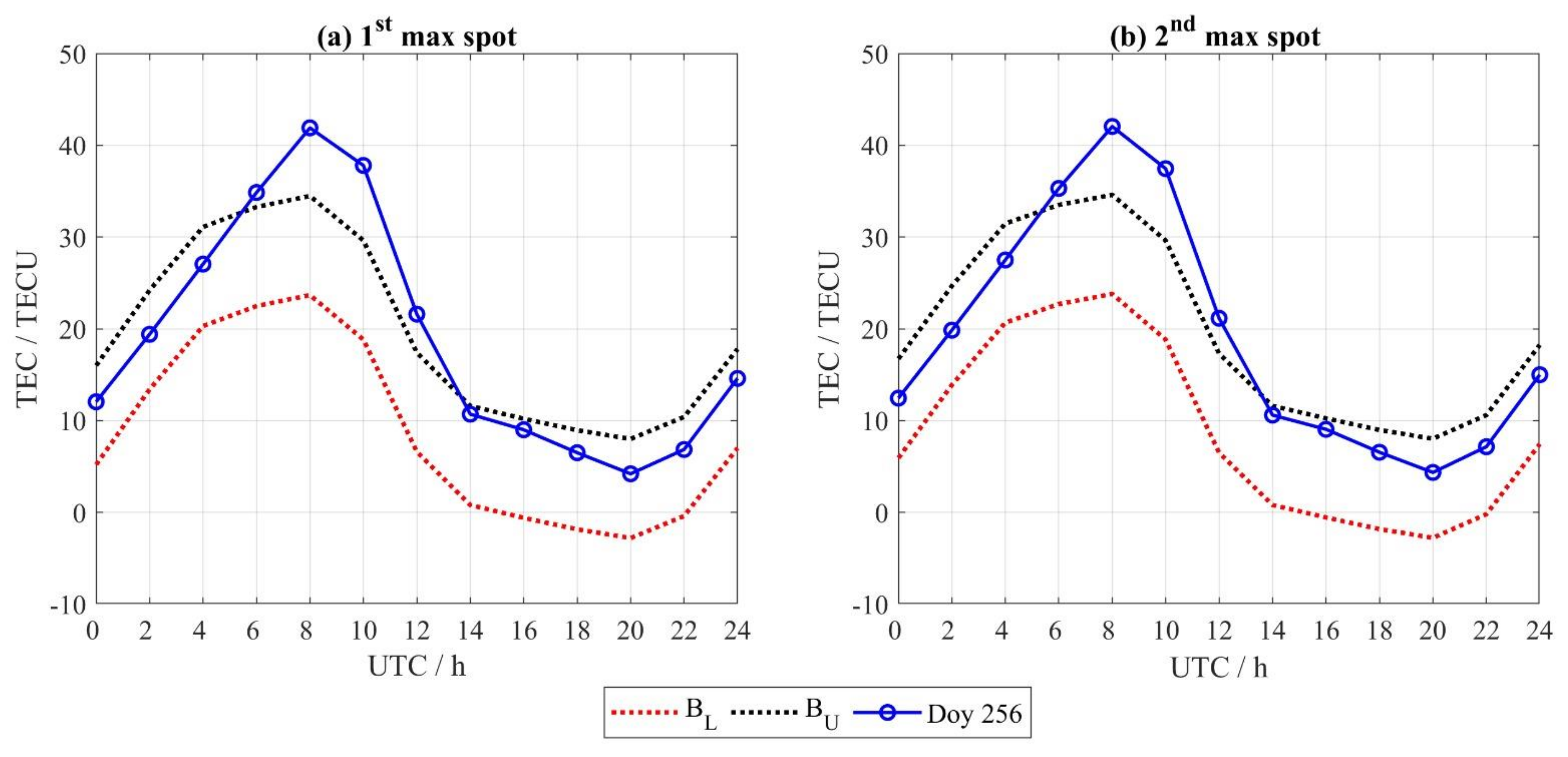
| BL | Lower Bound |
| BU | Upper Bound |
| CCL | Carrier-to-Code Leveling |
| CODE | Center for Orbit Determination in Europe |
| CORS | Continuously Operating Reference Stations |
| DOY | Day Of the Year |
| Dst | Disturbance storm-time |
| EAD | Enhanced Average Difference |
| F10.7 | solar radio flux at 10.7 cm |
| GEC | Global Electric Circuit |
| GIMs | Global Ionosphere Maps |
| GNSS | Global Navigation Satellite System |
| HF | High-Frequency |
| HK | Hong Kong |
| HKT | Hong Kong Time |
| IAWs | Internal Atmospheric Waves |
| IGS | International GNSS Service |
| IPP | Ionospheric Pierce Point |
| IQR | InterQuartile Range |
| Kp | the geomagnetic Kp |
| LOS MNG NOAA-PSL | Line Of Sight mean of the nearest two grid points National Oceanic and Atmospheric Administration-Physical Sciences Laboratory |
| nT | nano Tesla |
| NWP | Northwest Pacific Ocean |
| R1 | lowest range limit |
| R2 | highest range limit |
| RIMs | Regional Ionosphere Maps |
| RTD | Range of ten Days |
| sfu | Solar Flux Unit |
| SLM | single-layer mapping |
| STEC | Slant Total Electron Content |
| TC | Tropical Cyclone |
| TEC | Total Electron Content |
| TECU | Total Electron Content Unit |
| VTEC | vertical Total Electron Content |
| Time (HKT) | Days of September | DOY | Geographical Location (Degree) | Classification | Maximum Sustained wind Speed (km/h) | |
|---|---|---|---|---|---|---|
| 2:00 | 11 | 254 | 14.0 N | 142.6 E | Severe Typhoon | 165 |
| 8:00 | 11 | 254 | 14.0 N | 141.2 E | Super Typhoon | 185 |
| 14:00 | 11 | 254 | 13.9 N | 139.8 E | Super Typhoon | 205 |
| 20:00 | 11 | 254 | 13.7 N | 138.6 E | Super Typhoon | 220 |
| 8:00 | 12 | 255 | 13.9 N | 136.2 E | Super Typhoon | 240 |
| 2:00 | 13 | 256 | 14.4 N | 132.5 E | Super Typhoon | 240 |
| 2:00 | 14 | 257 | 15.2 N | 127.9 E | Super Typhoon | 240 |
| 20:00 | 14 | 257 | 17.4 N | 124.1 E | Super Typhoon | 240 |
| 23:00 | 14 | 257 | 17.7 N | 123.2 E | Super Typhoon | 250 |
| 2:00 | 15 | 258 | 18.0 N | 122.3 E | Super Typhoon | 250 |
| 5:00 | 15 | 258 | 18.0 N | 121.3 E | Super Typhoon | 230 |
| 11:00 | 15 | 258 | 18.3 N | 120.1 E | Super Typhoon | 195 |
| Date | DOY | Start Time | Peak Time | End Time | Class |
|---|---|---|---|---|---|
| Sept. 11 | DOY 254 | 7:56 | 7:59 | 8:01 | B |
| Sept. 12 | DOY 255 | NA | NA | NA | NA |
| Sept. 13 | DOY 256 | 17:56 | 17:58 | 18:02 | A |
| Sept. 14 | DOY 257 | NA | NA | NA | NA |
| Sept. 15 | DOY 258 | NA | NA | NA | NA |
| Sept. 16 | DOY 259 | 4:34 | 4:35 | 4:36 | A |
| Sept. 17 | DOY 260 | NA | NA | NA | NA |
Publisher’s Note: MDPI stays neutral with regard to jurisdictional claims in published maps and institutional affiliations. |
© 2021 by the authors. Licensee MDPI, Basel, Switzerland. This article is an open access article distributed under the terms and conditions of the Creative Commons Attribution (CC BY) license (http://creativecommons.org/licenses/by/4.0/).
Share and Cite
Freeshah, M.; Zhang, X.; Şentürk, E.; Adil, M.A.; Mousa, B.G.; Tariq, A.; Ren, X.; Refaat, M. Analysis of Atmospheric and Ionospheric Variations Due to Impacts of Super Typhoon Mangkhut (1822) in the Northwest Pacific Ocean. Remote Sens. 2021, 13, 661. https://doi.org/10.3390/rs13040661
Freeshah M, Zhang X, Şentürk E, Adil MA, Mousa BG, Tariq A, Ren X, Refaat M. Analysis of Atmospheric and Ionospheric Variations Due to Impacts of Super Typhoon Mangkhut (1822) in the Northwest Pacific Ocean. Remote Sensing. 2021; 13(4):661. https://doi.org/10.3390/rs13040661
Chicago/Turabian StyleFreeshah, Mohamed, Xiaohong Zhang, Erman Şentürk, Muhammad Arqim Adil, B. G. Mousa, Aqil Tariq, Xiaodong Ren, and Mervat Refaat. 2021. "Analysis of Atmospheric and Ionospheric Variations Due to Impacts of Super Typhoon Mangkhut (1822) in the Northwest Pacific Ocean" Remote Sensing 13, no. 4: 661. https://doi.org/10.3390/rs13040661