
Quiet Ionospheric D-Region (QIonDR) Model Based on VLF/LF Observations

 ,
,  , , and
Abstract
:
1. Introduction
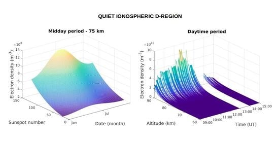
- long-term variations (about 11 years) in solar radiations during solar cycle;
- seasonal variations (due to Earth’s revolution);
- daytime periodical changes; and
- sudden mid- and short-term influences
2. Methodology
2.1. Midday Periods
2.1.1. VLF/LF Signal Processing
- 1
- Determination of the amplitude of signal in a quiet state before an X-ray flare XF. To find this value for both VLF/LF signals, we consider three time bins of length (in our processing we use s) within a time window of a few minutes before the signal perturbation. The amplitude is defined as the minimum of median values of recorded amplitudes in each bin, while the maximal absolute deviation of the recorded amplitudes in the considered bins from the median value is used as a figure for its absolute error d. In the following, we use “d” for the absolute error and “” to denote the difference between the amplitudes at two different times during the disturbance and quiet state.
- 2
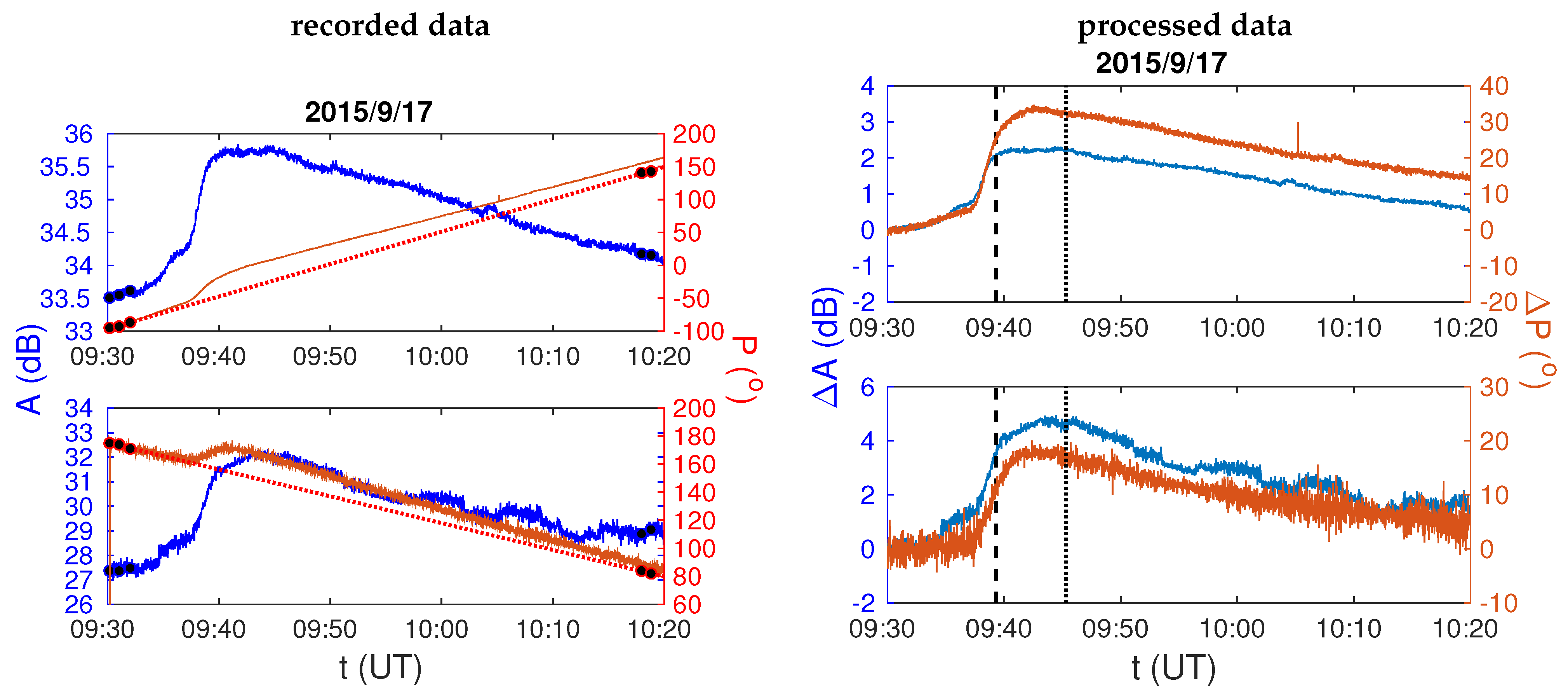
- Determination of the reference phase of a signal during an X-ray flare XF. The recorded phase of a VLF/LF signal represents the phase deviation of the considered signal with respect to the phase generated at the receiver. For this reason, the recorded phase has a component of constant slope that should be removed. A linear fit is performed through five points, three before the signal perturbation and two at the end of the considered observation interval, is performed. Phase values at these points are determined in the same way as in the procedure for amplitude estimation as described in point 1). For each time bin , we compute the median value of phase samples. Furthermore, the largest deviation of phase values within each bin is used to estimate the absolute error d of the reference phase.It is worth noting that disturbances induced by a solar X-ray flare can last from several tenth of minutes to over one hour. For this reason, quiet conditions can be different before and after disturbances. In addition, it is possible that some sudden events or some technical problem affect at least one signal in a time interval starting after the one used in this study. For instance, in Figure 2, we show a visible increase in the “quiet” visible increase in the “quiet” phase of about 15 and 5 for the DHO and ICV signals, respectively.
- 3
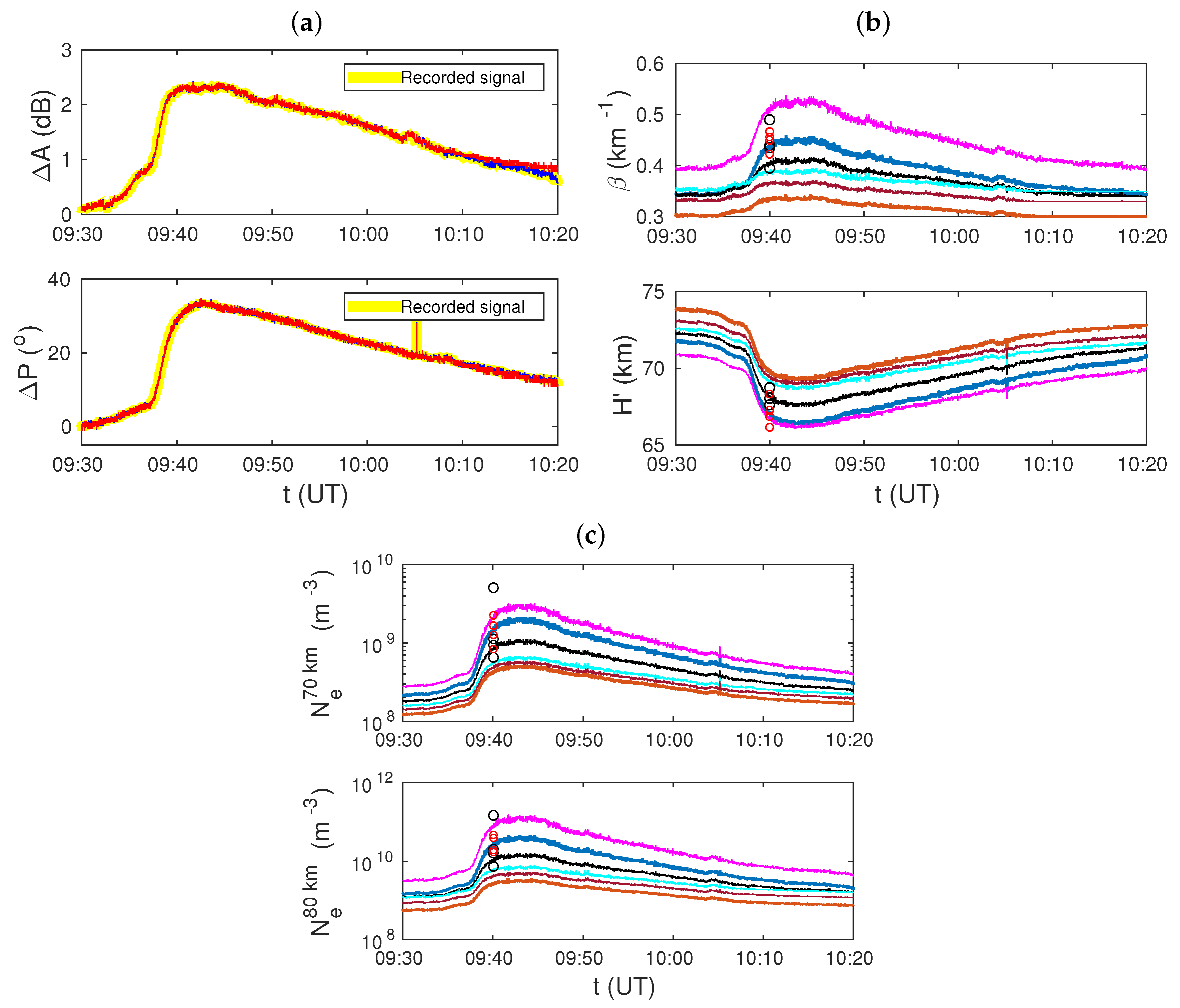
- Determination of differences in the amplitude and phase of the signal during a disturbance induced by a solar X-ray flare XF in state with respect to quiet conditions. To avoid any dependence of results on the selection of time, we perform twice the analysis of changes in the signal parameters with respect to the initial, unperturbed state, by selecting two different times which are emphasized by vertical dashed and dotted lines in right panels in Figure 2 displaying time evolutions of the amplitude () and phase () changes for both signals during the disturbance induced by the solar X-ray flare occurred on 17 September 2015.The absolute errors d and absolute errors d of amplitudes and , and d and d of phases and , respectively, are determined as for the quiet state, i.e.: (1) we calculate , , and as median values in two bins of width s around times and ; (2) we define absolute errors d and d, and d and d in terms of maximal absolute deviations of the corresponding quantities within the bins. The total absolute errors are obtained as follows:where .
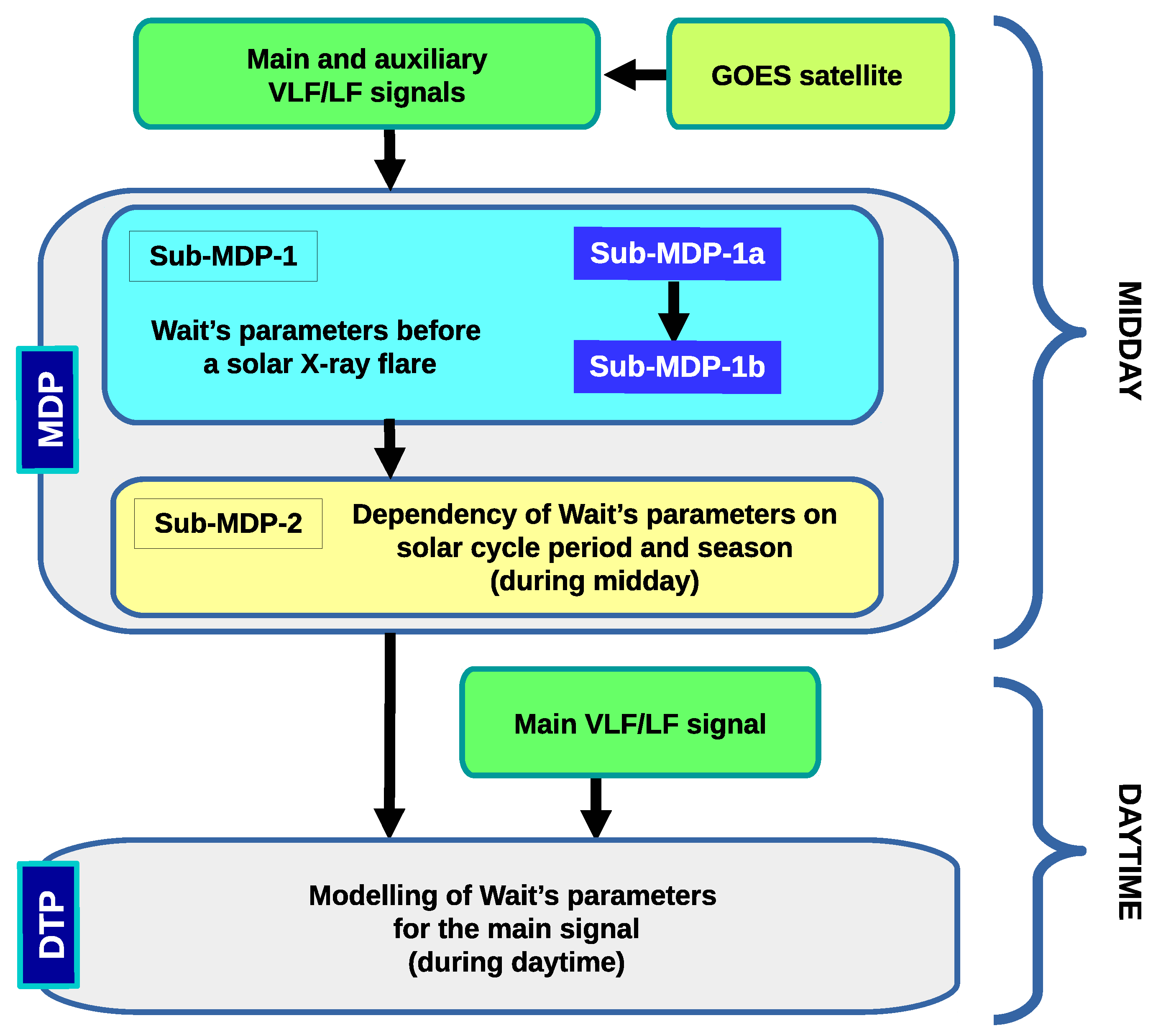
2.1.2. Modeling
- Sub-MDP-1:
- Estimation of Wait’s parameters in quiet conditions before a solar X-ray flare. As can be seen in Figure 1 this procedure consists of two following sub-procedures:
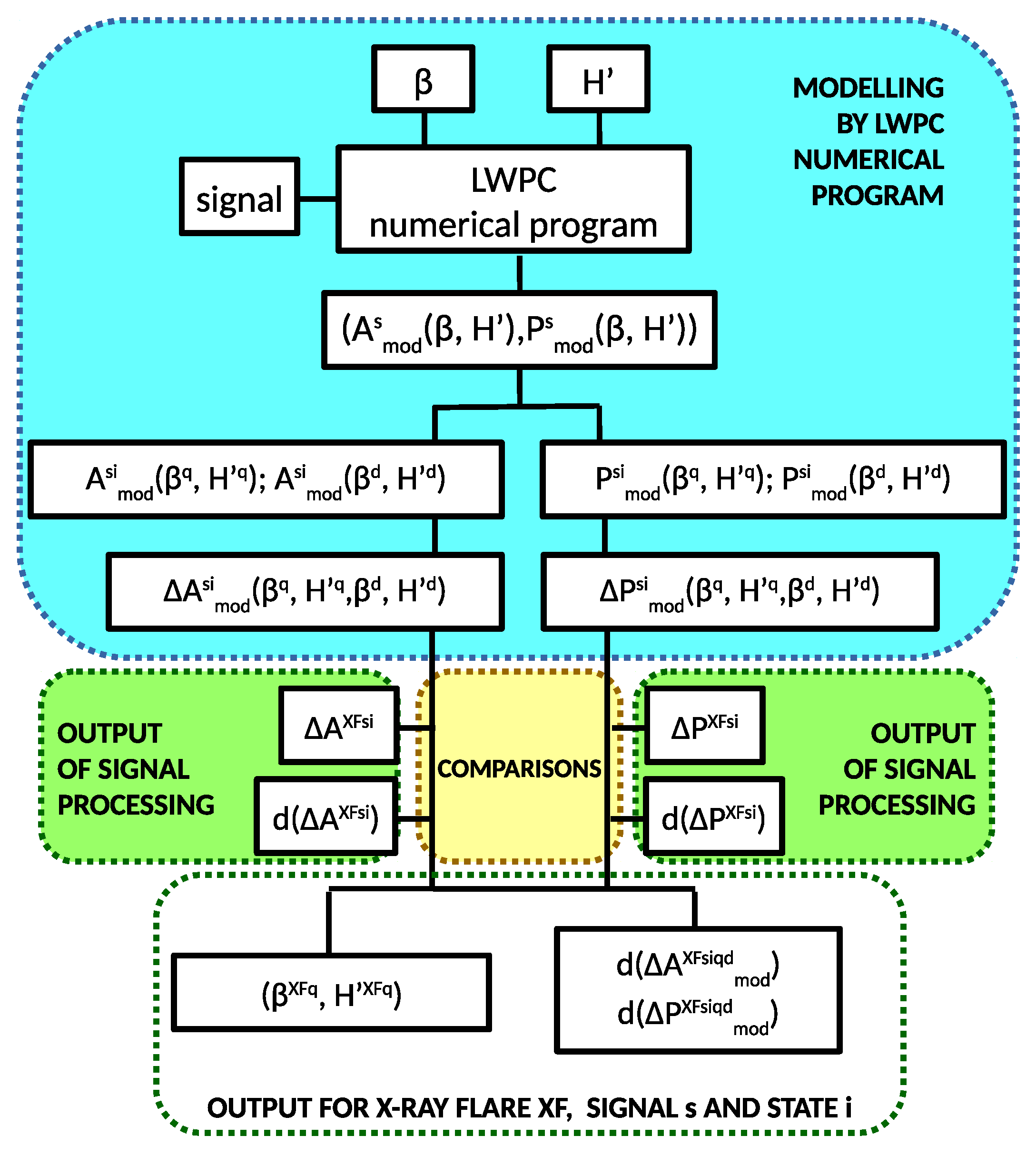
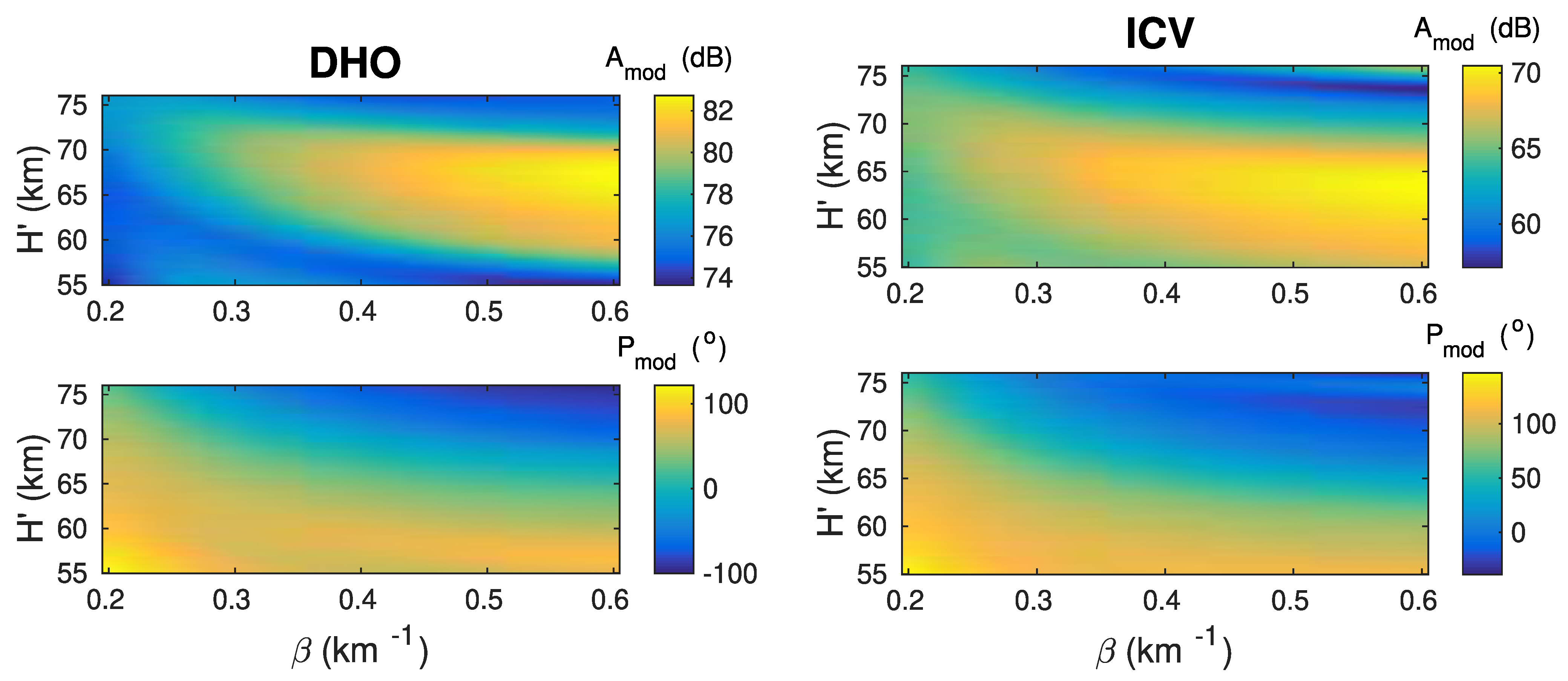
- Sub-MDP-1a. This sub-procedure provides values of Wait’s parameters in the quiet ionosphere for which the amplitude and phase changes are similar to the corresponding recorded values, and , respectively. It is based on determination of changes in two sets of the modeled amplitude and phase of the signal s, and their deviations from the corresponding recorded values and for the signal s and disturbed state i. These sets, representing the modeled quiet and disturbed states, q and d, respectively, are performed in simulations of the considered VLF/LF signal propagation using LWPC numerical model developed by the Space and Naval Warfare Systems Center, San Diego, CA, USA [22]. The input parameters of this numerical model are Wait’s parameters “sharpness” and signal reflection height, while the modeled amplitude and phase are its output (see the diagram in Figure 3).According to the results presented in literature (see References [26,27,31,33,34,35]), Wait’s parameters can be considered within intervals 0.2 km–0.6 km for , and 55 km–76 km for , where the quiet conditions can be described within intervals 0.2 km–0.45 km for , and 68 km–76 km for . To model the parameter values representing a disturbed state d, and , given those describing a quiet state q, we use conditions and which are based on many studies [26,27,31]. In the following, we use these intervals with steps of 0.01 km and 0.1 km, respectively, as input in the LWPC numerical program.The first output of the Sub-MDP-1a are the pairs of Wait’s parameters referring to the quiet state before a solar X-ray flare XF for which the LWPC model can calculate the amplitude and phase differences for both main (m) and auxiliary (a) signals () and for both disturbed state () that satisfy the conditions:where and are the absolute errors in the recorded signal characteristics.The second output of Sub-MDP-1a are errors in modeling, e.g., the absolute deviations of the modeled changes in the amplitude and phase from their recorded values: and . Both outputs are used in Sub-MDP-1b.
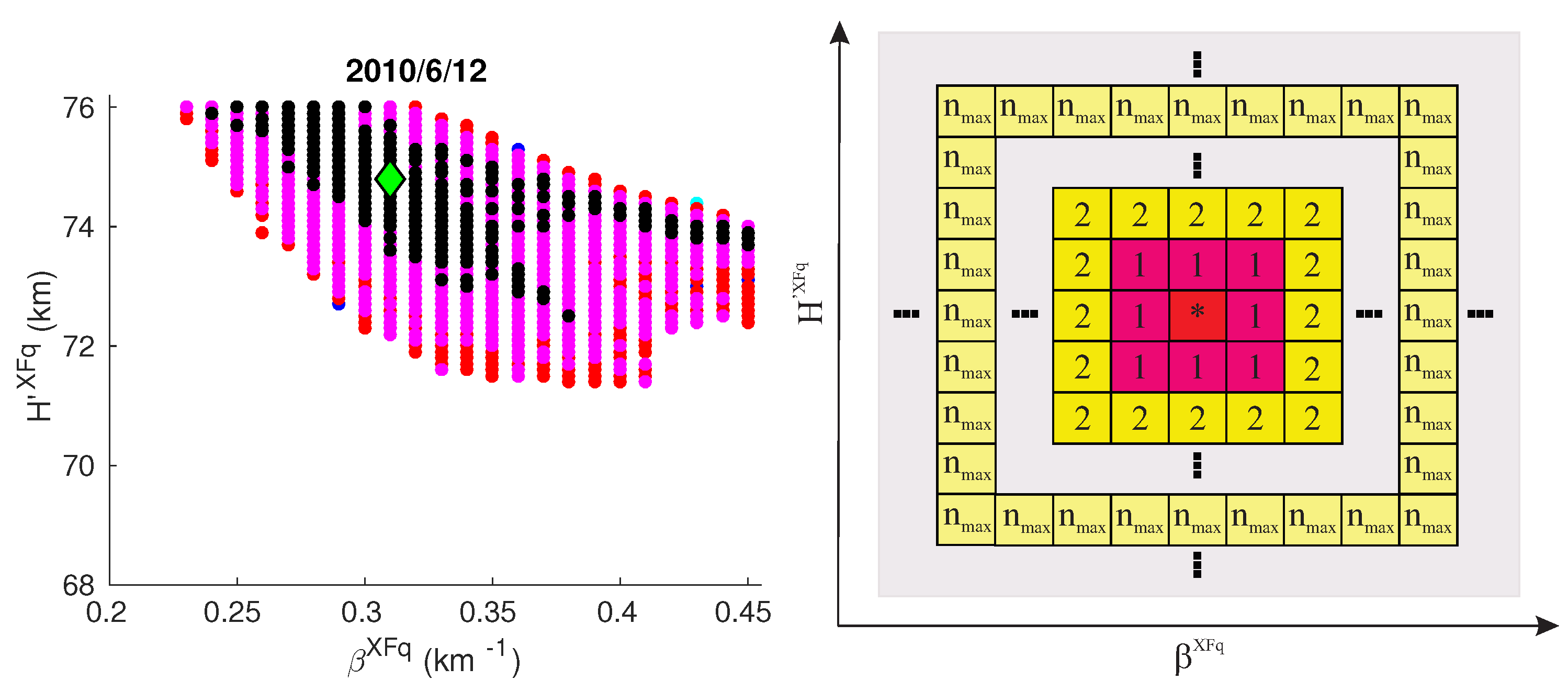
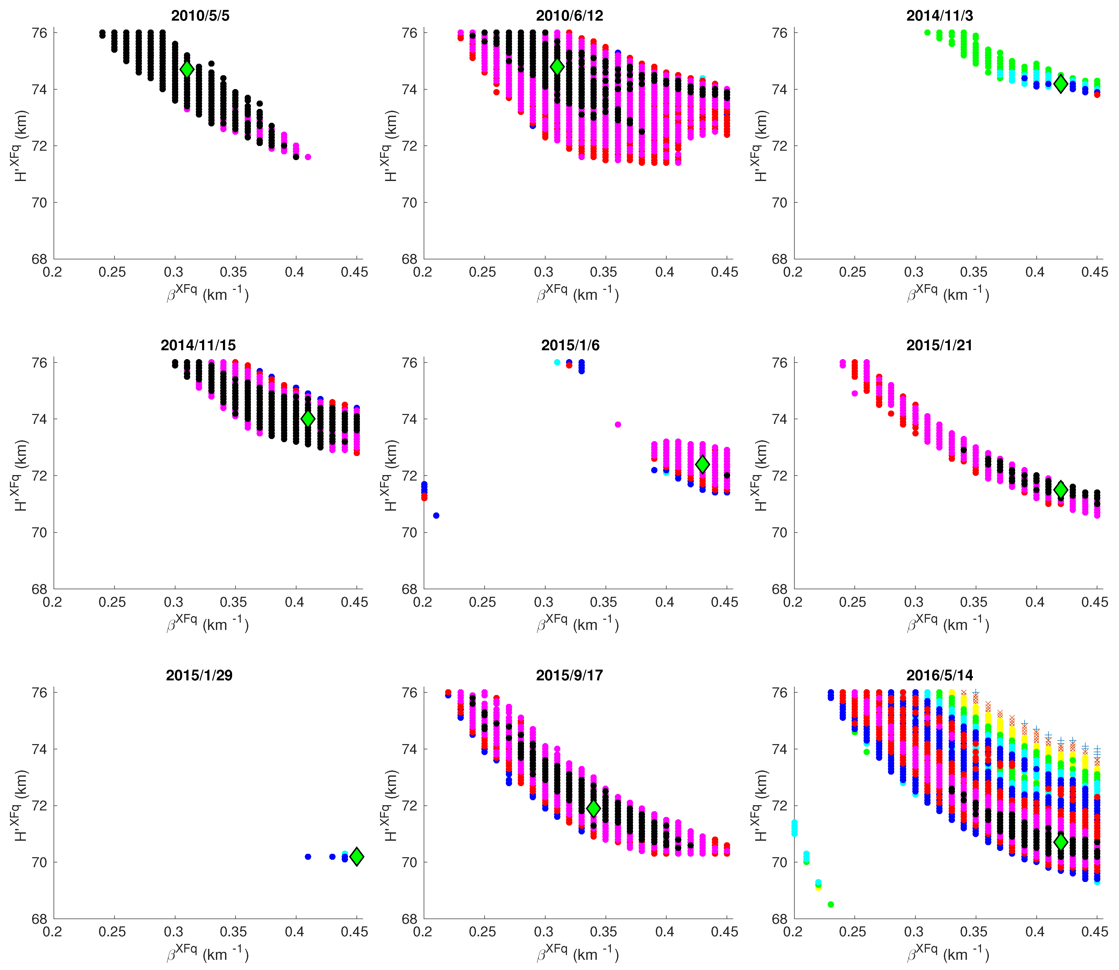
- Sub-MDP-1b. The goal of this sub-procedure is to find the pair of Wait’s parameters ,, from those extracted in Sub-MDP-1a, which provides the best agreement between the modeled and measured amplitude and phase changes of the VLF/LF signals. To do that, we analyze both the observation and modeling absolute errors, i.e., and , for observations and and for modeling. These values are used to quantify the observed and modeled weights for each extracted pair of Wait’s parameters. Details about the estimations of these weights are provided in Appendix A, while an example of representation of the extracted pairs in the 2D Wait’s parameter space is shown in the left panel of Figure 4. Each pair of Wait’s parameters is represented as a point. The color of points describes their observation and modeling precisions. To find points (i.e., pairs of Wait’s parameters) which best model the amplitude and phase changes, the region around each candidate point is analyzed as follows. The weight of each point, describing the overall observation and modeling precisions, is computed as the product of observed and modeled weights, i.e., .Furthermore, the weight is introduced to quantify the influence of each point within the region around the candidate point. This weight is defined aswhere is the distance between the quiet states q and k which refer to pairs and , respectively.The total weight for the pair is computed as:Finally, the pair of Wait’s parameters describing the quiet D-region before a solar X-ray flare XF, which provides the best agreement of the considered modeled and observed amplitude and phase changes, is obtained as the pair with the largest total weight . The estimation errors and of these parameters are obtained from distribution of pairs which satisfy conditions (6) and (7). For instance, the error for are computed as follows. For the pair represented by green diamonds in Figure 4, the interval is estimated by taking the smaller and larger values of estimates, for the given . In the same way, we estimate the error for .
- Sub-MDP-2:
- Modeling of Wait’s parameters in terms of sunspot number and season. The aim of this subroutine is to model the behaviour of Wait’s parameters by fitting the pair. This requires a deeper understanding of the X-ray influences on the D-region. During quiet conditions, the solar hydrogen Ly radiation has a dominant influence on ionization processes in the ionospheric D-region (see, for example, Reference [45]). The intensity of this radiation varies periodically during the solar cycle and its variation depends on the sunspot number. Because of that, we use the smoothed daily sunspot number to represent the intensity of the incoming solar radiation in the Earth’s atmosphere. The intensity of this radiation decreases with the solar zenith angle due to larger attenuations in the atmosphere above the considered locations. Generally, the zenith angle changes are due to seasonal and‘daily variations. However, this study focuses on time intervals around middays which allows us to assume that the seasonal changes represent the zenith angle variations. We introduce the seasonal parameter where DOY is the day of year. This parameter has values between 0 and 1. Some authors report on possible influences of the geomagnetic field on the Wait’s parameter [38,46]. However, this is is more pronounced at polar and near polar areas due to shapes of geomagnetic lines that allows charge particle influences on the ionospheric properties. As this study is focused on the low and mid latitude ionosphere, we neglect these effects.Dependencies of Wait’s parameters at midday on solar cycle and seasonal variations can be given as functions:andThese relations are not general and have yet to be determined for the location of interest and the time to which the recorded data refer to.
2.2. Daytime Variations of Ionospheric Parameters
2.2.1. VLF/LF Signal Processing
2.2.2. Modeling
3. Studied Area and Considered Events
3.1. Remote Sensing of Lower Ionosphere
3.2. Considered X-ray Flares
4. Results and Discussion
- 1
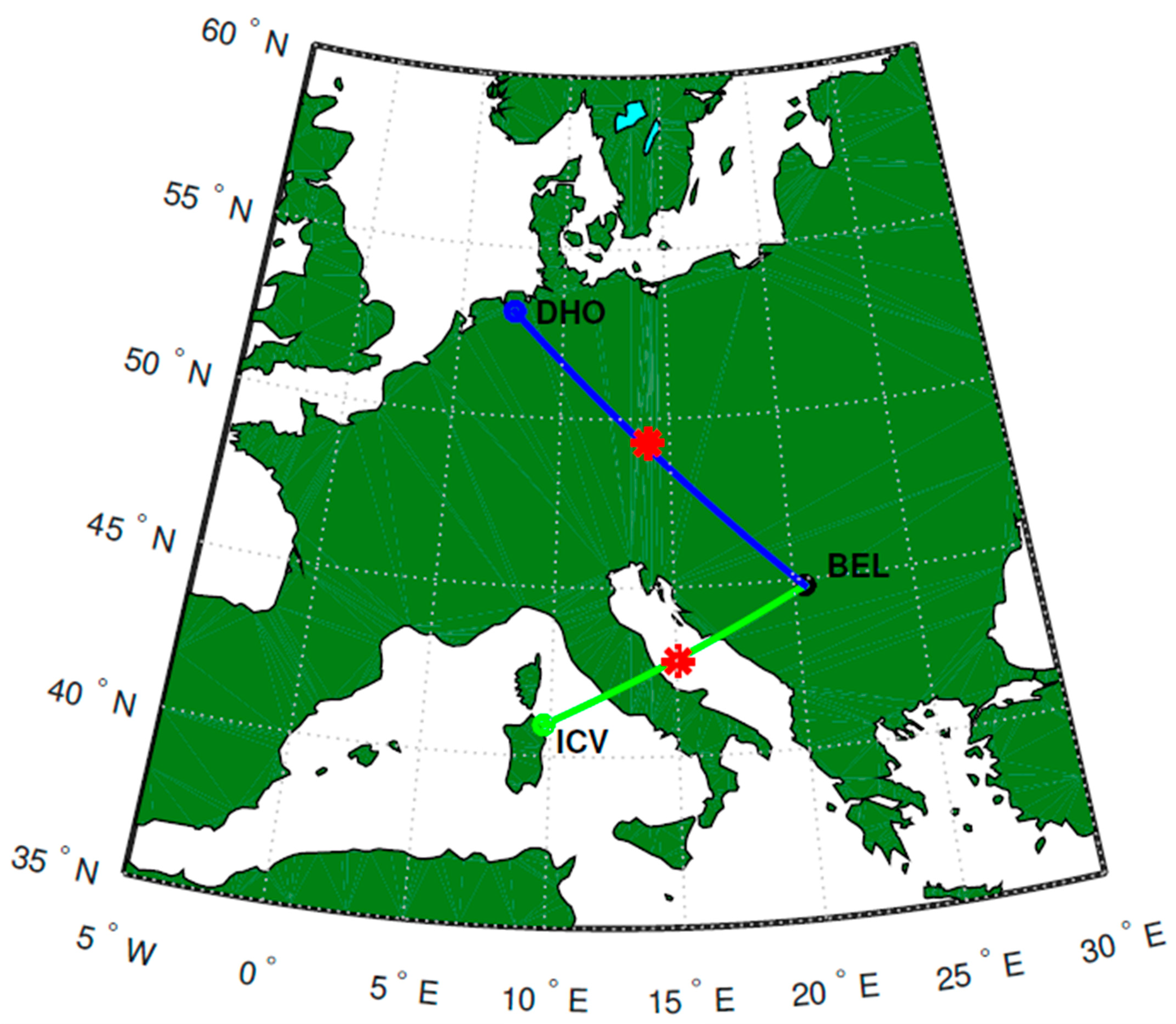
- Modeling the ionospheric parameters in midday periods over the part of Europe included within the location of transmitted signals (Sardinia, Italy, for the ICV signal) and (Lower Saxony, Germany for the DHO signal) and the receiver in Belgrade, Serbia, with respect to the daily smoothed sunspot number and season. This part consists of the following steps:
- Determination of dependencies of the midday Wait’s parameters, and , and the electron density, , from parameters that describe the solar activity and Earth’s motion: the smoothed daily sunspot number , and parameter describing seasonal variations.
- 2
- Modeling of daytime variations of ionospheric parameters for a particular day. This procedure consists of:
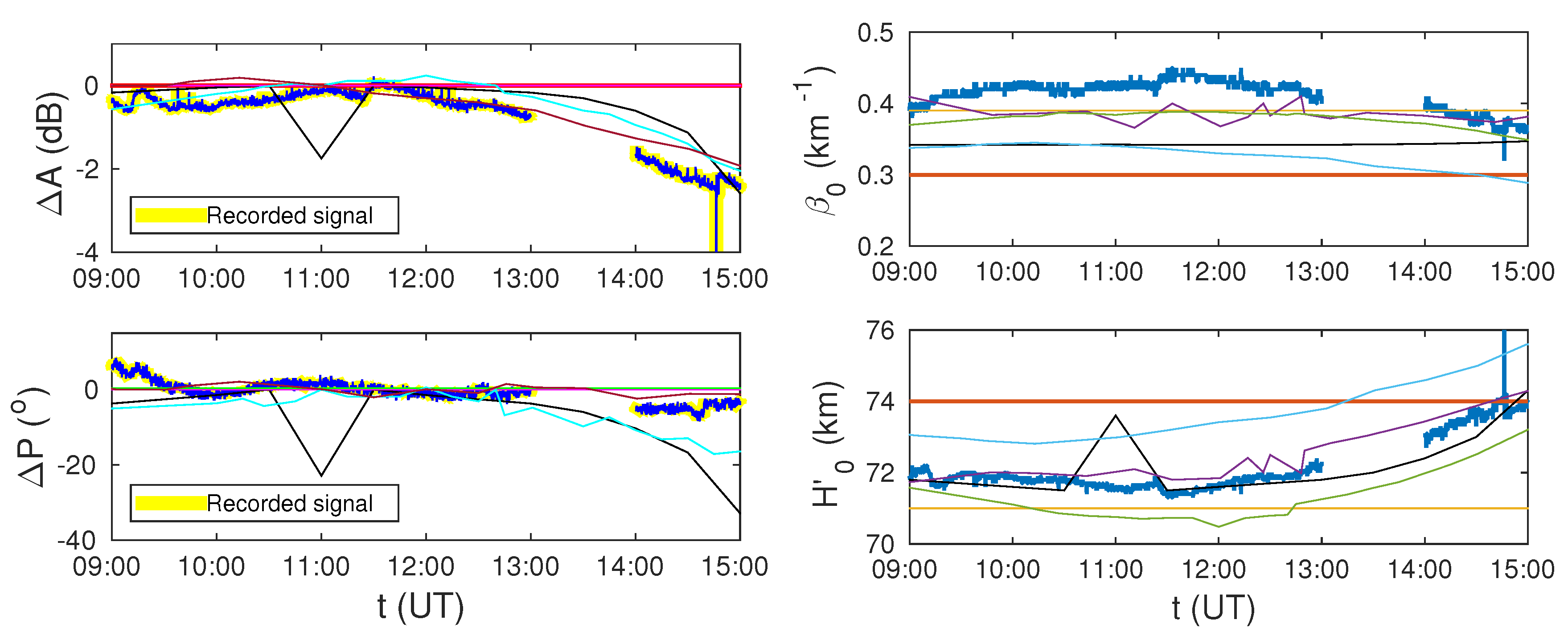
- Modeling of time evolutions of Wait’s parameters from comparisons of the recorded and modeled amplitude and phase changes with respect to their values in the midday.
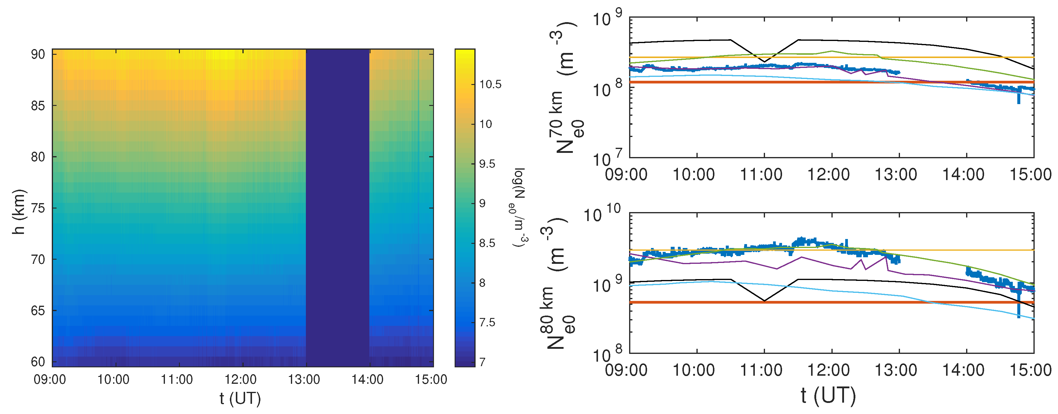
- Modeling of the electron density time evolution for the D-region heights during daytime.
4.1. Modeling of the DHO and ICV Signal Amplitudes and Phases by the LWPC Numerical Program
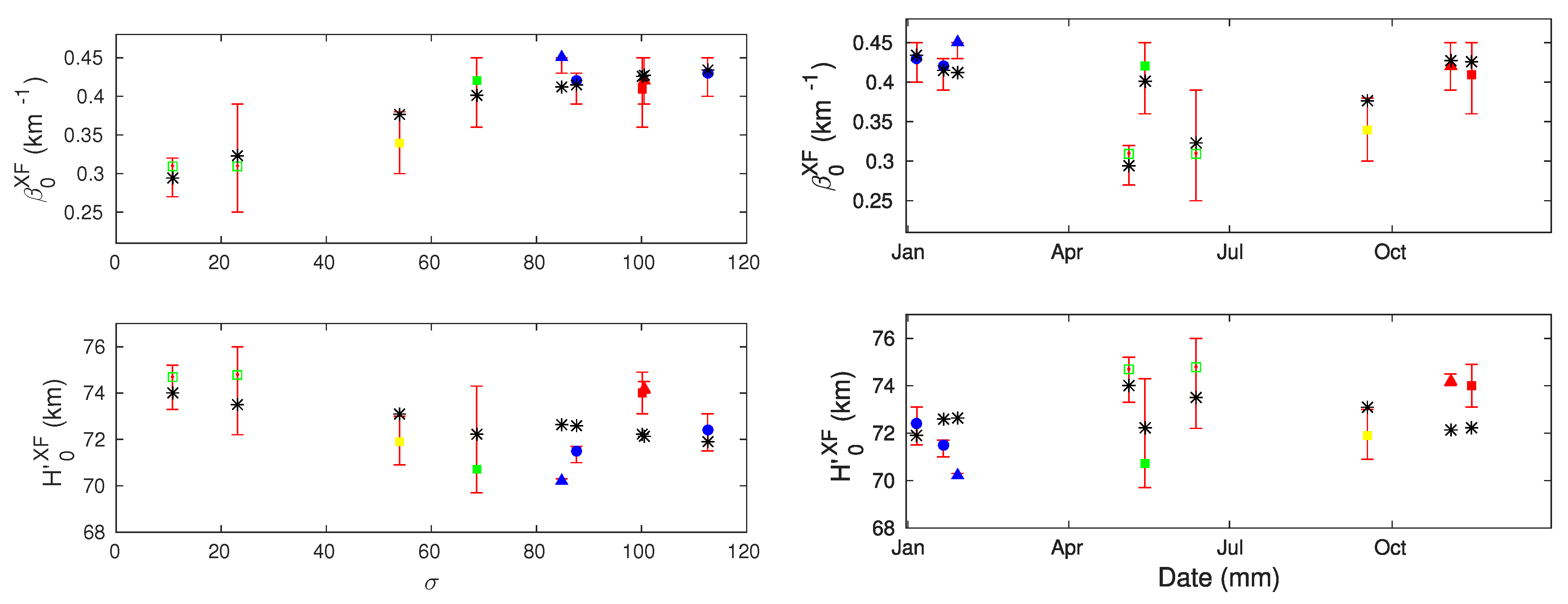
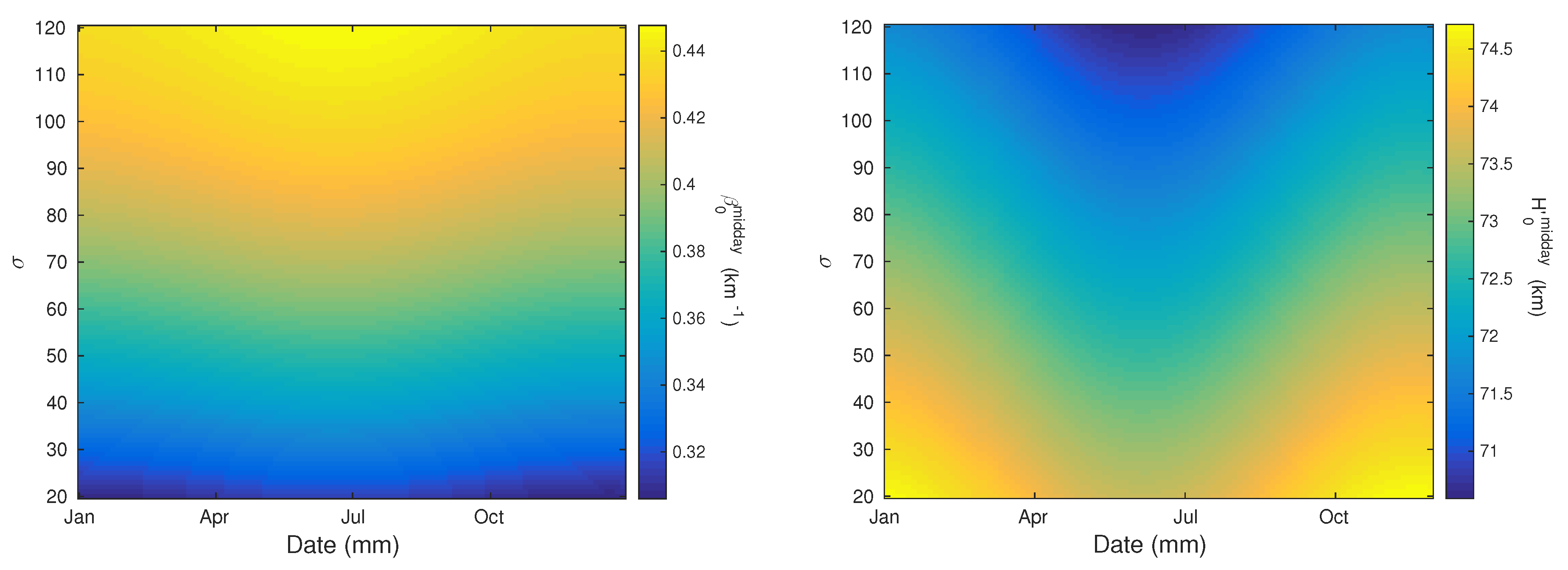
4.2. Midday Values—Solar Cycle and Seasonal Variations
- Determination of pairs which describe quiet states before the considered X-ray flares (Section 4.2.1).
- Determination of dependencies of Wait’s parameters and the electron density in midday quiet conditions on and (Section 4.2.2).
4.2.1. Determination of Pairs
4.2.2. Wait’s Parameters and Electron Density in Quiet Conditions
4.3. Daytime Variations
5. Conclusions
- A new procedure for estimation of Wait’s parameters and electron density. It is divided in two parts: (1) determination of dependencies of these parameters on the smoothed daily sunspot number and season at midday, and (2) determination of time evolution of these parameters during daytime;
- Estimation of Wait’s parameters and electron density over the part of Europe included within the location of the transmitted signals (Sardinia, Italy, for the ICV signal) and (Lower Saxony, Germany for the DHO signal) and the receiver in Belgrade, Serbia. The obtained results show variations in which inclusion in different analyses of more events or time periods will allow more realistic comparisons and statistic studies;
- Analytical expressions for dependencies of Wait’s parameters on the smoothed daily sunspot number and seasonal parameter valid over the studied area.
- Time periods during quiet conditions or during disturbances that do not affect the assumed horizontal uniformity of the observed D-region (for example, the midday periods during the influence of solar X-ray flares),
- VLF/LF signals in which propagation paths between transmitters and receivers are relatively short, and
- Mid- and low-latitude areas where the spatial variations of the magnetic field are not significant in the given conditions.
Author Contributions
Funding
Data Availability Statement
Acknowledgments
Conflicts of Interest
Sample Availability
Appendix A
- Weight . The relative errors of the recorded signal amplitude and phase are obtained as a ratio of their absolute errors and the corresponding observed changes:The total relative error of the observed changes related to a solar X-ray flare XF is given by:The observational weight for an X-ray flare XF is defined as reciprocal value of the total relative error:
- Weight . This weight is computed for Wait’s parameters in a quiet state q for which AT LEAST one corresponding pair is such that Equations (6) and (7) are satisfied for both signals s and both states i. In the case there are more pairs with the quite state q, the relative error is defined as:The modeled weight is calculated as:
References
- Kintner, P.M.; Ledvina, B.M. The ionosphere, radio navigation, and global navigation satellite systems. Adv. Space Res. 2005, 35, 788–811. [Google Scholar] [CrossRef]
- Meyer, F. Performance requirements for ionospheric correction of low-frequency SAR data. IEEE Trans. Geosci. Remote Sens. 2011, 49, 3694–3702. [Google Scholar] [CrossRef]
- Jakowski, N.; Stankov, S.M.; Klaehn, D. Operational space weather service for GNSS precise positioning. Ann. Geophys. 2005, 23, 3071–3079. [Google Scholar] [CrossRef]
- Benevides, P.; Nico, G.; Catalão, J.; Miranda, P.M.A. Bridging InSAR and GPS Tomography: A New Differential Geometrical Constraint. IEEE Trans. Geosci. Remote Sens. 2016, 54, 697–702. [Google Scholar] [CrossRef]
- Benevides, P.; Nico, G.; Catalão, J.; Miranda, P.M.A. Analysis of Galileo and GPS Integration for GNSS Tomography. IEEE Trans. Geosci. Remote Sens. 2017, 55, 1936–1943. [Google Scholar] [CrossRef]
- Su, K.; Jin, S.; Hoque, M.M. Evaluation of Ionospheric Delay Effects on Multi-GNSS Positioning Performance. Remote Sens. 2019, 11, 171. [Google Scholar]
- Yang, H.; Yang, X.; Zhang, Z.; Sun, B.; Qin, W. Evaluation of the Effect of Higher-Order Ionospheric Delay on GPS Precise Point Positioning Time Transfer. Remote Sens. 2020, 12, 2129. [Google Scholar] [CrossRef]
- Farzaneh, S.; Forootan, E. A Least Squares Solution to Regionalize VTEC Estimates for Positioning Applications. Remote Sens. 2020, 12, 3545. [Google Scholar] [CrossRef]
- Miranda, P.M.A.; Mateus, P.; Nico, G.; Catalão, J.; Tomé, R.; Nogueira, M. InSAR Meteorology: High-Resolution Geodetic Data Can Increase Atmospheric Predictability. Geophys. Res. Lett. 2019, 46, 2949–2955. [Google Scholar] [CrossRef] [Green Version]
- Nina, A.; Nico, G.; Odalović, O.; Čadež, V.; Drakul, M.T.; Radovanović, M.; Popović, L. GNSS and SAR Signal Delay in Perturbed Ionospheric D-Region During Solar X-ray Flares. IEEE Geosci. Remote Sens. Lett. 2020, 17, 1198–1202. [Google Scholar] [CrossRef]
- Zhao, J.; Zhou, C. On the optimal height of ionospheric shell for single-site TEC estimation. GPS Solut. 2018, 22, 48. [Google Scholar] [CrossRef]
- Nava, B.; Coïsson, P.; Radicella, S. A new version of the NeQuick ionosphere electron density model. J. Atmos. Solar-Terr. Phys. 2008, 70, 1856–1862. [Google Scholar] [CrossRef]
- Scherliess, L.; Schunk, R.W.; Sojka, J.J.; Thompson, D.C.; Zhu, L. Utah State University Global Assimilation of Ionospheric Measurements Gauss-Markov Kalman filter model of the ionosphere: Model description and validation. J. Geophys. Res.-Space 2006, 111, 1–19. [Google Scholar] [CrossRef] [Green Version]
- Silber, I.; Price, C. On the Use of VLF Narrowband Measurements to Study the Lower Ionosphere and the Mesosphere–Lower Thermosphere. Surv. Geophys. 2017, 38, 407–441. [Google Scholar] [CrossRef] [Green Version]
- Nina, A.; Pulinets, S.; Biagi, P.; Nico, G.; Mitrović, S.; Radovanović, M.; Popović, L. Variation in natural short-period ionospheric noise, and acoustic and gravity waves revealed by the amplitude analysis of a VLF radio signal on the occasion of the Kraljevo earthquake (Mw = 5.4). Sci. Total Environ. 2020, 710, 136406. [Google Scholar] [CrossRef] [PubMed]
- Kumar, S.; NaitAmor, S.; Chanrion, O.; Neubert, T. Perturbations to the lower ionosphere by tropical cyclone Evan in the South Pacific Region. J. Geophys. Res. Space 2017, 122, 8720–8732. [Google Scholar] [CrossRef]
- Nina, A.; Radovanović, M.; Milovanović, B.; Kovačević, A.; Bajčetić, J.; Popović, L. Low ionospheric reactions on tropical depressions prior hurricanes. Adv. Space Res. 2017, 60, 1866–1877. [Google Scholar] [CrossRef] [Green Version]
- Biagi, P.F.; Maggipinto, T.; Righetti, F.; Loiacono, D.; Schiavulli, L.; Ligonzo, T.; Ermini, A.; Moldovan, I.A.; Moldovan, A.S.; Buyuksarac, A.; et al. The European VLF/LF radio network to search for earthquake precursors: Setting up and natural/man-made disturbances. Nat. Hazards Earth Syst. Sci. 2011, 11, 333–341. [Google Scholar]
- Inan, U.S.; Lehtinen, N.G.; Moore, R.C.; Hurley, K.; Boggs, S.; Smith, D.M.; Fishman, G.J. Massive disturbance of the daytime lower ionosphere by the giant γ-ray flare from magnetar SGR 1806-20. Geophys. Res. Lett. 2007, 34, 8103. [Google Scholar] [CrossRef] [Green Version]
- Tanaka, Y.T.; Raulin, J.P.; Bertoni, F.C.P.; Fagundes, P.R.; Chau, J.; Schuch, N.J.; Hayakawa, M.; Hobara, Y.; Terasawa, T.; Takahashi, T. First Very Low Frequency Detection of Short Repeated Bursts from Magnetar SGR J1550-5418. Astrophys. J. Lett. 2010, 721, L24–L27. [Google Scholar] [CrossRef]
- Bajčetić, J.; Nina, A.; Čadež, V.M.; Todorović, B.M. Ionospheric D-Region Temperature Relaxation and Its Influences on Radio Signal Propagation After Solar X-Flares Occurrence. Thermal Sci. 2015, 19, S299–S309. [Google Scholar] [CrossRef]
- Ferguson, J.A. Computer Programs for Assessment of Long-Wavelength Radio Communications, Version 2.0; Space and Naval Warfare Systems Center: San Diego, CA, USA, 1998. [Google Scholar]
- Marshall, R.A.; Wallace, T.; Turbe, M. Finite-Difference Modeling of Very-Low-Frequency Propagation in the Earth-Ionosphere Waveguide. IEEE Trans. Antennas Propag. 2017, 65, 7185–7197. [Google Scholar] [CrossRef]
- Rapoport, Y.; Grimalsky, V.; Fedun, V.; Agapitov, O.; Bonnell, J.; Grytsai, A.; Milinevsky, G.; Liashchuk, A.; Rozhnoi, A.; Solovieva, M.; et al. Model of the propagation of very low-frequency beams in the Earth–ionosphere waveguide: Principles of the tensor impedance method in multi-layered gyrotropic waveguides. Ann. Geophys. 2020, 38, 207–230. [Google Scholar] [CrossRef] [Green Version]
- Morfitt, D.G.; Shellman, C.H. MODESRCH, an Improved Computer Program for Obtaining ELF/VLF Mode Constants in an EARTH-Ionosphere Waveguide; Naval Electronics Laboratory Center: San Diego, CA, USA, 1976. [Google Scholar]
- McRae, W.M.; Thomson, N.R. Solar flare induced ionospheric D-region enhancements from VLF phase and amplitude observations. J. Atmos. Solar Terr. Phys. 2004, 66, 77–87. [Google Scholar] [CrossRef]
- Thomson, N.R.; Rodger, C.J.; Clilverd, M.A. Large solar flares and their ionospheric D region enhancements. J. Geophys. Res. Space 2005, 110, A06306. [Google Scholar] [CrossRef] [Green Version]
- Žigman, V.; Grubor, D.; Šulić, D. D-region electron density evaluated from VLF amplitude time delay during X-ray solar flares. J. Atmos. Solar Terr. Phys. 2007, 69, 775–792. [Google Scholar] [CrossRef]
- Grubor, D.P.; Šulić, D.M.; Žigman, V. Classification of X-ray solar flares regarding their effects on the lower ionosphere electron density profile. Ann. Geophys. 2008, 26, 1731–1740. [Google Scholar] [CrossRef] [Green Version]
- Basak, T.; Chakrabarti, S.K. Effective recombination coefficient and solar zenith angle effects on low-latitude D-region ionosphere evaluated from VLF signal amplitude and its time delay during X-ray solar flares. Astrophys. Space Sci. 2013, 348, 315–326. [Google Scholar]
- Nina, A.; Čadež, V. Electron production by solar Ly-α line radiation in the ionospheric D-region. Adv. Space Res. 2014, 54, 1276–1284. [Google Scholar]
- Poulsen, W.L.; Bell, T.F.; Inan, U.S. The scattering of VLF waves by localized ionospheric disturbances produced by lightning-induced electron precipitation. J. Geophys. Res. Space 1993, 98, 15553–15559. [Google Scholar] [CrossRef]
- Han, F.; Cummer, S.A.; Li, J.; Lu, G. Daytime ionospheric D region sharpness derived from VLF radio atmospherics. J. Geophys. Res.-Space Phys. 2011, 116, 5314. [Google Scholar]
- Thomson, N.R. Experimental daytime VLF ionospheric parameters. J. Atmos. Solar Terr. Phys. 1993, 55, 173–184. [Google Scholar] [CrossRef]
- McRae, W.M.; Thomson, N.R. VLF phase and amplitude: Daytime ionospheric parameters. J. Atmos. Solar Terr. Phys. 2000, 62, 609–618. [Google Scholar] [CrossRef]
- Thomson, N.R.; Rodger, C.J.; Clilverd, M.A. Daytime D region parameters from long-path VLF phase and amplitude. J. Geophys. Res.-Space 2011, 116, 11305. [Google Scholar] [CrossRef] [Green Version]
- Gross, N.C.; Cohen, M.B. VLF Remote Sensing of the D Region Ionosphere Using Neural Networks. J. Geophys. Res. Space 2020, 125, e2019JA027135. [Google Scholar] [CrossRef]
- Davis, R.M.; Berry, L.A. A Revised Model of the Electron Density in the Lower Ionosphere; Technical Report TR III-77; Defense Communications Agency Command Control Technical Center: Washington, DC, USA, 1977. [Google Scholar]
- Todorović Drakul, M.; Čadež, V.M.; Bajčetić, J.; Popović, L.Č; Popović, D.B.; Nina, A. Behaviour of electron content in the ionospheric D-region during solar X-ray flares. Serb. Astron. J. 2016, 193, 11–18. [Google Scholar] [CrossRef]
- Srećković, V.; Šulić, D.; Vujičić, V.; Jevremović, D.; Vyklyuk, Y. The effects of solar activity: Electrons in the terrestrial lower ionosphere. J. Geograph. Inst. Cvijic 2017, 67, 221–233. [Google Scholar] [CrossRef]
- Morgan, R.R. World-Wide VLF Effective Conductivity Map; Westinghouse Electric: Cranberry Township, PA, USA, 1968. [Google Scholar]
- Wait, J.R.; Spies, K.P. Characteristics of the Earth-Ionosphere Waveguide for VLF Radio Waves; NBS Technical Note: Boulder, CO, USA, 1964.
- Belrose, J.S.; Burke, M.J. Study of the Lower Ionosphere using Partial Reflection: 1. Experimental Technique and Method of Analysis. J. Geophys. Res. 1964, 69, 2799–2818. [Google Scholar] [CrossRef]
- Kane, J. Re-evaluation of ionospheric electron densities and collision frequencies derived from rocket measurements of refractive index and attenuation. J. Atmos. Terr. Phy. 1961, 23, 338–347. [Google Scholar] [CrossRef]
- Mitra, A.P. (Ed.) Ionospheric Effects of Solar Flares. Astrophysics and Space Science Library; Springer Nature: Cham, Switzerland, 1974; Volume 46. [Google Scholar]
- Ferguson, J.A. Ionospheric Profiles for Predicting Nighttime VLF/LF Propagation; Technical report; Naval Ocean Systems Center: San Diego, CA, USA, 1980. [Google Scholar]
- Kumar, A.; Kumar, S. Solar flare effects on D-region ionosphere using VLF measurements during low- and high-solar activity phases of solar cycle 24. Earth Planets Space 2018, 70, 29. [Google Scholar] [CrossRef]
- Hayes, L.A.; Gallagher, P.T.; McCauley, J.; Dennis, B.R.; Ireland, J.; Inglis, A. Pulsations in the Earth’s Lower Ionosphere Synchronized With Solar Flare Emission. J. Geophys. Res.-Space 2017, 122, 9841–9847. [Google Scholar] [CrossRef] [Green Version]
- Cohen, M.B.; Inan, U.S.; Paschal, E.W. Sensitive Broadband ELF/VLF Radio Reception With the AWESOME Instrument. IEEE Trans. Geosci. Remote Sens. 2010, 48, 3–17. [Google Scholar] [CrossRef]
- Nina, A.; Čadež, V.M.; Bajčetić, J.; Mitrović, S.T.; Popović, L.Č. Analysis of the Relationship Between the Solar X-ray Radiation Intensity and the D-Region Electron Density Using Satellite and Ground-Based Radio Data. Solar Phys. 2018, 293, 64. [Google Scholar] [CrossRef]
- Ammar, A.; Ghalila, H. Estimation of nighttime ionospheric D-region parameters using tweek atmospherics observed for the first time in the North African region. Adv. Space Res. 2020, 66, 2528–2536. [Google Scholar] [CrossRef]
- Bilitza, D. IRI the International Standard for the Ionosphere. Adv. Radio Sci. 2018, 16, 1–11. [Google Scholar] [CrossRef] [Green Version]
- Thomson, N.R.; Clilverd, M.A.; Rodger, C.J. Midlatitude ionospheric D region: Height, sharpness, and solar zenith angle. J. Geophys. Res. Space 2017, 122, 8933–8946. [Google Scholar] [CrossRef] [Green Version]


 QIonDR;
  LWPC default [22];
  IRI [52];
  Thomson et al., 2005 [27];
  Han et al., 2011 [33];
  McRae and Thomson, 2000 [35];
  Thomson et al., 2017 [53].
QIonDR; LWPC default [22]; IRI [52]; Thomson et al., 2005 [27]; Han et al., 2011 [33]; McRae and Thomson, 2000 [35]; Thomson et al., 2017 [53].
Thomson et al., 2017 [53].
QIonDR; LWPC default [22]; IRI [52]; Thomson et al., 2005 [27]; Han et al., 2011 [33]; McRae and Thomson, 2000 [35]; Thomson et al., 2017 [53]. QIonDR; LWPC default [22]; IRI [52]; Thomson et al., 2005 [27]; Han et al., 2011 [33]; McRae and Thomson, 2000 [35]; Thomson et al., 2017 [53].
QIonDR; LWPC default [22]; IRI [52]; Thomson et al., 2005 [27]; Han et al., 2011 [33]; McRae and Thomson, 2000 [35]; Thomson et al., 2017 [53].
QIonDR; LWPC default [22]; IRI [52]; Thomson et al., 2005 [27]; Han et al., 2011 [33]; McRae and Thomson, 2000 [35]; Thomson et al., 2017 [53]. QIonDR; LWPC default [22]; IRI [52]; Thomson et al., 2005 [27]; McRae and Thomson, 2000 [35]; Thomson et al., 2017 [53]; o Grubor et al., 2008 [29]; o McRae and Thomson, 2004 [26].
QIonDR; LWPC default [22]; IRI [52]; Thomson et al., 2005 [27]; McRae and Thomson, 2000 [35]; Thomson et al., 2017 [53]; o Grubor et al., 2008 [29]; o McRae and Thomson, 2004 [26].
QIonDR; LWPC default [22]; IRI [52]; Thomson et al., 2005 [27]; McRae and Thomson, 2000 [35]; Thomson et al., 2017 [53]; o Grubor et al., 2008 [29]; o McRae and Thomson, 2004 [26].

| Flare XF | Date | Time (UT) | Flare Class | () | () | () |
|---|---|---|---|---|---|---|
| F1 | 5 May 2010 | 11:37 | C8.8 | 33.79 | 27.88 | 5.91 |
| F2 | 12 June 2010 | 09:20 | C6.1 | 35.39 | 31.25 | 4.14 |
| F3 | 3 November 2014 | 11:23 | M2.2 | 64.84 | 58.61 | 6.23 |
| F4 | 15 November 2014 | 11:40 | M3.2 | 53.57 | 51.35 | 2.22 |
| F5 | 6 January 2015 | 11:40 | C9.7 | 72.05 | 65.76 | 6.29 |
| F6 | 21 January 2015 | 11:32 | C9.9 | 69.25 | 62.88 | 6.37 |
| F7 | 29 January 2015 | 11:32 | M2.1 | 53.07 | 50.65 | 2.42 |
| F8 | 17 September 2015 | 09:34 | M1.1 | 50.31 | 44.28 | 6.03 |
| F9 | 14 May 2016 | 11:28 | C7.4 | 37.50 | 35.31 | 2.19 |
| Flare XF | |||||||||
|---|---|---|---|---|---|---|---|---|---|
| No | (km) | (km) | (km) | (km) | (km) | (km) | |||
| F1 | 0.31 | 74.7 | 0.01 | 0.04 | 0.5 | 1.4 | 104.0 | 10.7 | 0.3452 |
| F2 | 0.31 | 74.8 | 0.08 | 0.06 | 1.2 | 2.6 | 103.5 | 23.1 | 0.4493 |
| F3 | 0.42 | 74.2 | 0.03 | 0.03 | 0.3 | 0.2 | 5.6 | 100.5 | 0.8438 |
| F4 | 0.41 | 74.0 | 0.04 | 0.05 | 0.9 | 0.9 | 154.5 | 100.1 | 0.8767 |
| F5 | 0.43 | 72.4 | 0.02 | 0.03 | 0.7 | 0.9 | 29.7 | 112.6 | 0.0164 |
| F6 | 0.42 | 71.5 | 0.01 | 0.03 | 0.2 | 0.5 | 56.8 | 87.6 | 0.0575 |
| F7 | 0.45 | 70.2 | 0.00 | 0.02 | 0.1 | 0.1 | 1.4 | 84.8 | 0.0795 |
| F8 | 0.34 | 71.9 | 0.04 | 0.04 | 1.1 | 1.0 | 115.9 | 54.0 | 0.7151 |
| F9 | 0.42 | 70.7 | 0.03 | 0.06 | 3.6 | 1.0 | 111.5 | 68.6 | 0.3699 |
Publisher’s Note: MDPI stays neutral with regard to jurisdictional claims in published maps and institutional affiliations. |
© 2021 by the authors. Licensee MDPI, Basel, Switzerland. This article is an open access article distributed under the terms and conditions of the Creative Commons Attribution (CC BY) license (http://creativecommons.org/licenses/by/4.0/).
Share and Cite
Nina, A.; Nico, G.; Mitrović, S.T.; Čadež, V.M.; Milošević, I.R.; Radovanović, M.; Popović, L.Č. Quiet Ionospheric D-Region (QIonDR) Model Based on VLF/LF Observations. Remote Sens. 2021, 13, 483. https://doi.org/10.3390/rs13030483
Nina A, Nico G, Mitrović ST, Čadež VM, Milošević IR, Radovanović M, Popović LČ. Quiet Ionospheric D-Region (QIonDR) Model Based on VLF/LF Observations. Remote Sensing. 2021; 13(3):483. https://doi.org/10.3390/rs13030483
Chicago/Turabian StyleNina, Aleksandra, Giovanni Nico, Srđan T. Mitrović, Vladimir M. Čadež, Ivana R. Milošević, Milan Radovanović, and Luka Č. Popović. 2021. "Quiet Ionospheric D-Region (QIonDR) Model Based on VLF/LF Observations" Remote Sensing 13, no. 3: 483. https://doi.org/10.3390/rs13030483