PointNet++ Network Architecture with Individual Point Level and Global Features on Centroid for ALS Point Cloud Classification

Abstract

Airborne laser scanning (ALS) point cloud has been widely used in the fields of ground powerline surveying, forest monitoring, urban modeling, and so on because of the great convenience it brings to people’s daily life. However, the sparsity and uneven distribution of point clouds increases the difficulty of setting uniform parameters for semantic classification. The PointNet++ network is an end-to-end learning network for irregular point data and highly robust to small perturbations of input points along with corruption. It eliminates the need to calculate costly handcrafted features and provides a new paradigm for 3D understanding. However, each local region in the output is abstracted by its centroid and local feature that encodes the centroid’s neighborhood. The feature learned on the centroid point may not contain relevant information of itself for random sampling, especially in large-scale neighborhood balls. Moreover, the centroid point’s global-level information in each sample layer is also not marked. Therefore, this study proposed a modified PointNet++ network architecture which concentrates the point-level and global features on the centroid point towards the local features to facilitate classification. The proposed approach also utilizes a modified Focal Loss function to solve the extremely uneven category distribution on ALS point clouds. An elevation- and distance-based interpolation method is also proposed for the objects in ALS point clouds which exhibit discrepancies in elevation distributions. The experiments on the Vaihingen dataset of the International Society for Photogrammetry and Remote Sensing and the GML(B) 3D dataset demonstrate that the proposed method which provides additional contextual information to support classification achieves high accuracy with simple discriminative models and new state-of-the-art performance in power line categories.

1. Introduction

The innovations in dense stereo- or multiview photogrammetry, Light Detection and Ranging (LiDAR), synthetic aperture radar, and structure from motion have broadened the availability of 3D point cloud data, which are widely used in many fields, including automatic navigation [1], 3D city management [2] and 3D building reconstruction [3]. Collected images of real 3D scenes may be occluded and are thus complex. Compare with 2D images which lose depth information and relative positions between two or more objects in the real world, 3D point cloud provides an opportunity for a better understanding of the surrounding environment for machines. Point cloud data contain rich semantic information and have high density and high precision. Hence, they have become one of the main data types used in 3D object recognition research. Point cloud data can enrich the understanding and analysis of complex 3D scenes. 3D laser scanners can measure objects without touching them and quickly obtain massive point cloud data, which include spatial coordinates and the color and reflection intensity of objects. These devices operate under any weather condition and achieve high precision, density, and efficiency. These unique advantages of 3D laser scanners provide 3D point cloud data with great application prospects and increase their market demand.

As a new surveying and mapping technology, airborne LiDAR technology can rapidly acquire large-scale and high-density ground information with relatively high precision; it has also been used in high-precision mapping, digital city reconstruction [4], forest monitoring [5], cultural heritage protection [6], natural disaster monitoring, and other fields [7].

Airborne laser scanning (ALS) point clouds have followed three characteristics: (1) Objects present large-scale variations between different categories, ranging from small spatial neighborhoods (cars, power lines) to large ones (buildings), such variations entail high requirements for data processing. (2) Many categories have evidence of geometric properties, e.g., tracts of roof and façade. (3) The objects in ALS point clouds exhibit discrepancies in elevation distributions [8]. The ALS point cloud classification is a difficult problem due to terrain complexity, scene’s clutter, overlapping in the vertical direction, and nonuniformity density distribution.

In 3D classification, the point cloud is divided into groups and then a label is assigned according to their type. This step is an important part of laser point cloud data processing. In one method for ALS point cloud classification, each point in a point set is regarded as an independent entity, and only a single-point local feature is used in classification [9]. However, single-point local feature classification is unstable for cases with a nonuniform point cloud density distribution, especially those involving complex scenes [10]. Another classification method introduces contextual information for ALS point cloud classification on the basis of single-point local features [11,12]. The method using handcrafted features and classifiers require the manual extraction of context features in advance, which need manual intervention in data processing, and consumes 70–80% of the whole processing time [13]. Meanwhile, low-dimensional handcrafted features have weak representation ability, and automated interpretation and knowledge discovery from 3D point cloud data remains challenging.

The recent research into 3D laser point cloud has already broken through traditional technical methods and has gradually been integrated into multiple disciplines (such as machine learning) [1,14,15]. With the outstanding performance of deep learning technology in target recognition, researchers have also extended it to 3D target recognition to improve the level of automation and intelligence. Convolutional neural networks (CNNs) have achieved great success on 2D image recognition tasks; however, input point sets are different from CNN inputs, which refer to data defined on regular grids with uniform constant density. Many studies have attempted to generate feature images for point clouds and then apply them to 2D CNNs for ALS point cloud classification. However, transforming unstructured 3D point sets into regular representation inevitability causes spatial information loss.

Qi proposed a deep learning framework called PointNet that consumes unordered and unstructured point clouds directly [16]. PointNet++ network was later developed to enable multiscale point feature learning [17]. Following the great success of PointNet and PointNet++ network, many PointNet-like architectures have been proposed; they include PointCNN [18], PointSift [19], D-FCN [20], PointLK [21], KPConv [22], PV-RCNN [23] and so on. PointNet++ has been used in 3D object classification, 3D part segmentation, and 3D scene segmentation and has a broad market.

Although PointNet++ has a higher generalization ability than PointNet, its usage in the classification of large-scale airborne point clouds in complex scenes is still challenging. The objects on ALS point clouds cannot be present in CAD models such as ModelNet40, which are small man-made objects containing fixed information and are free from occlusion and noise [17]. In module training, the process of splitting and sampling is inevitable on ALS point clouds. As ALS point clouds have their own characteristics listed above, a universal point cloud multitarget recognition method should be established, and the need for costly calculations in ALS point cloud classification should be eliminated.

Inspired by the success of PointNet++ network, we proposed a method which fully utilizes point clouds in an end-to-end manner. The proposed method allows us to identify unordered point sets with varying densities without needing us to design complicated handcrafted features. The main contributions of this work are summarized as follows:

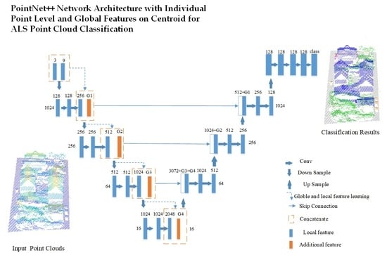
• The point-level and global information on the centroid point in the sample layer in the PointNet++ network is added to the local feature at multiple scales to extract other useful informative features to solve the uneven distribution of point clouds problem.
• One modified loss function based on focal loss function is proposed to solve the extremely uneven category distribution problem.
• The elevation- and distance-based interpolation method is proposed for objects in ALS point clouds that exhibit discrepancies in elevation distributions.
• In addition to a theoretical analysis, experimental evaluations are conducted using the Vaihingen 3D dataset of the International Society for Photogrammetry and Remote Sensing (ISPRS) and the GML(B) dataset.

2. Related Work

2.1. Using Handcrafted Features and Classifiers

Traditional point cloud classification methods are related to the estimation of single-point local features. In one strategy, only local geometry features are used, and each point in a point set is regarded as an independent entity. Antonarakis et al. used the 3D coordinates, elevation, and intensity of point clouds to classify forest and ground types on the basis of a supervised object-orientated approach [24]. Zhang et al. calculated the 13 features of 3D point clouds in terms of geometry, radiometry, topology, and echo characteristics and then utilized a support vector machine (SVM) to classify ALS point clouds [9]. However, classification methods that use single-point local features are unstable in cases involving nonuniform point cloud density distributions as they are influenced by classification noises and label inconsistencies [10].

Another strategy involves the derivation of suitable 3D descriptors, such as spin image descriptors [25], point feature histograms [26] and the signature of histograms of orientations [27]. Several approaches to 3D point cloud classification rely on 3D structure tensors, hence the proposal of the eigenvalue analysis method [28], which may derive a set of local 3D shape features. These methods usually need to calculate additional local geometry features, such as planarity, sphericity, and roughness, to use the local structural information in the original 3D space. When the scene is complex, this process is usually time-consuming and results in a high computation cost.

Mallet [29] classified full-waveform LiDAR data by using a pointwise multiclass SVM. Horvat designed three contextual filters for detecting overgrowing vegetation, small objects attached to planar surfaces, and small objects that do not belong to vegetation according to the nonlinear distribution characteristics on vegetation points [11,12]. Chehata used random forests for feature detection and classification of urban scenes collected by airborne laser scanning [30]. Niemeyer proposed a contextual classification method on the basis of conditional random field (CRF) [31]. This classification model was later extended, and the spatial and semantic contexts were incorporated into a hierarchical, high-order, two-layer CRF [12].

These existing methods are generally applied to specific scenes. They also have weak representation ability, and they require manual intervention. In complex ALS point cloud semantic classification, these methods are laborious, and their robustness is unsatisfactory. The automated, machine-assisted solutions are needed amidst the increasing volume, variety, and velocity of digital data.

2.2. Using Deep Features and Neural Networks

The development of computer vision research in the past decade has broadened the availability of 3D point cloud data. The unprecedented volume, variety, and velocity of digital data overwhelm the existing capacities to manage and translate data into actionable information. Traditional point cloud classification methods are almost always focused on the design of handcrafted features and use machine learning-based classification models to conduct classification [12]. Recently, deep learning methods have attracted increasing attention. Driven by the improvement of CNNs, available large-scale datasets, and high-performance computing resources, deep learning has enjoyed unprecedented popularity in recent years. The success of 2D CNNs in various image recognition tasks, such as image labeling, semantic segmentation, object detection, and target tracking, has also encouraged the application of these frameworks to 3D semantic classification. The straightforward extension of 2D CNNs to 3D classification is hampered when dealing with nonuniform and irregular point cloud features. In such a case, the process requires the transformation of input data into views or volumes so as to meet the requirements of image-based CNNs. Therefore, many deep learning approaches involve the transformation of 3D data into regular 2D images, and then back-projection of 2D labels to 3D point clouds; Therefore, the 3D semantic classification labels were generated [32].

Qi et al. combined two distinct network architectures of the multiview approach with volumetric methods to improve the classification results; in their work, the 3D object was rotated to generate different 3D orientations, and each individual orientation was processed individually by the same network to generate 2D representations [33]. Su et al. utilized different virtual cameras to recognize 3D shapes from a collection of their rendered views on 2D images and employed a multiview CNN to feed these images and thereby obtain the predicted categories [34]. Boulch et al. proposed a framework which feeds multiple 2D image views (or snapshots) of point clouds into a fully convolutional network; in this framework, point cloud labels are obtained through back-projection [35].

However, the convolution applied to regular data (image or volumeter) is not invariant to the permutation of input data. Nonetheless, these transformations of input data into views or volumes suffer from model complexity, computation cost and high space requirements as the storage and computation cost grows cubically with the grid resolution. Pictures may easily be affected by weather conditions, lighting, shooting angle, and images only have plane features and thus lack spatial information. Hence, one cannot realize real 3D scene classification, and exploring the efficient used CNNs in 3D data is still needed.

2.3. PointNet and PointNet++ Network

The PointNet network serves as the foundation of point-based classification methods and has thus become a hotspot for point cloud classification. The PointNet network is an end-to-end learning network for irregular point data that is highly robust to small input point perturbations along with corruption. This network eliminates the need to calculate costly handcrafted features and thereby provides a new paradigm for 3D understanding. The PointNet network also has the potential to train point clouds without requiring parameters that are specific to objects in ALS data; hence, it achieves high efficiency and effectiveness [13]. Relative to volumetric models, the PointNet model reduces computation costs and memory by over 88% and 80%, respectively. Hence, it is widely preferred in portable and mobile devices.

PointNet has shown encouraging results for the automatic classification of ALS data, and many PointNet-like architectures have been proposed. PointNet only uses local and global information and thus lacks local context information [36]. Therefore, many scholars have proposed improved algorithms.

PointNet++ is a hierarchical neural network based on PointNet. Features at different scales are concatenated, and multiscale features are formed. The three key layers in PointNet++ are the sampling layer, grouping layer, and PointNet layer. The sampling layer uses farthest point sampling (FPS) to select a set of points from the input points which defines the centroids of local regions. Local region sets are constructed in the grouping layer by finding “neighboring” points around the centroids. Then, a mini- PointNet abstracts the sets of local points or features into higher-level representations. Several state-of-the-art techniques have been proposed to improve the performance of the PointNet++ network. These techniques can be divided into two types: multiscale grouping (MSG) methods and multiresolution grouping (MRG) methods. MSG methods apply grouping layers with different scales to capture multiscale patterns. The features learned at different scales are concatenated for subsequent processing. MSG methods are computationally expensive because they run PointNet for every centroid point at a large scale and select many centroid points at the lowest level; therefore, the time cost is significant. MRG methods are more computationally efficient than MSG methods because they avoid feature extraction in large-scale neighborhoods at the lowest levels.

Although PointNet++ achieves satisfactory performance in many tasks, its drawbacks still require the development of appropriate solutions. For the feature aggregation of local regions, the max pooling operation is implemented in the PointNet++ network, but this method is heuristic and insufficient without learnable parameters [33,37]. To address the above problems, Wang et al. put forward the dynamic graph CNN(DGCNN) which incorporates local neighborhood information by concatenating the centroid points features with the feature difference between their k-nearest neighbors and then followed by multilayer perceptron (MLP) and max pooling operation. However, this method only considers the relationship between centroid points and the neighbors’ points, and the information it collects is still limited because of the use of a simple mas pooling operation [38]. Zhao et al. proposed the adaptive feature adjustment module in the PointWeb network to connect and explore all pairs of points in a region [39]. PointCNN sorts the points into a potentially canonical order and applies convolution to the points. To use the orientation information of neighborhood points, scholars proposed a directionally constrained fully convolutional neural network (D-FCN), which searches the nearest neighborhood points in each of the eight evenly divided directions [20]. In sum, the method does not consider individual point-level and global information, and it does not embed the characteristics of ALS point clouds to further improve performance. In this work, the point-level and global information of centroid point is added to support classification, and the characteristics of ALS point cloud which exhibit discrepancies in elevation distributions is also used. We also proposed a modified focal loss function and conducted an experiment on two datasets. The proposed method is shown in the following section.

3. Materials and Methods

3.1. Point-Level and Global Information

The PointNet++ network uses iterative FPS to choose a subset of points. Each local region in an output is abstracted by its centroid and local feature that encodes the centroid’s neighborhoods. However, when analyzing the learned information carefully, the feature learned on the centroid point may not contain relevant information, especially in large-scale neighborhood balls. The airborne point cloud density distribution is uneven, especially in the intersect band. Besides, sampling all points in neighborhood balls is not realistic as it wastes memory and is inefficient. This defect presents a challenge in setting the radius size in the PointNet++ network. Figure 1 demonstrates PointNet++ in which MSG is used on the features learned on the centroid points.

As shown in Figure 1, the centroid point is not selected. Hence, the feature vector in each radius does not contain centroid point information itself. Figure 2 demonstrates the same situation in which MRG is applied.

Figure 2b shows that the spatial or spectral attributes of the centroid point itself are lost. The global information of the centroid points is also lost. As shown in Figure 2c, the individual point-level and global features of the centroid point are concatenated to the local features to extract information further.

The absence of point-level and global information may result in incorrect semantic classification. Therefore, the current study proposes a method that merges the point-level and global information of centroids and the local information in the PointNet++ network. The Vaihingen dataset processing is used as an example to illustrate the proposed network. The architecture of the proposed network is shown in Figure 3.

As shown in Figure 3, the MLP layer size number is larger for ALS point cloud classification than for other tasks, such as object classification, part segmentation, and indoor segmentation. ALS point cloud classification is complex and requires the collection of rich information. In Figure 3, the orange box shown with parameters G1, G2, G3, and G4 on top represent the point-level and global information, which is concatenated to the local features to capture useful information. The interpolated feature at each level is concatenated along with skip-linked features from the abstraction level, and fully connection and ReLU layers are adopted to capture each point feature vector, and a fully connected layer is used on the last upsampling layer.

All the points in the test can be inputted directly into the model without any preprocessing because of the fully convolutional nature of the proposed model. As for the addition of point-level and global information, the method could reduce the adverse influence on the nonuniformity of point cloud density distribution. The architecture can also revert to the PointNet++ network when the orange block is removed in Figure 3.

3.2. Modified Focal Loss Function

Category distribution is extremely uneven in ALS point clouds, as deduced from the number of points in each category. The training efficiency is low when most locations easily become negative, in which case useful learning signals are not provided. The negative values in turn overwhelm the training process and lead to model degradation. In the effort to avoid oversampling and undersampling, the common method is to increase the sampling rate in small category data so as to improve performance. Another approach is to reset the weight so that the algorithm pays close attention to small categories. The focal loss function aims to solve the uneven category issue. This function prevents the vast number of easy negatives from overwhelming the detector during training, and it has been widely used in image feature recognition and seldom on 3D point clouds processing. The focal loss function is modified from the cross-entropy function and is written as

$$\mathrm{FL}(p_t)=-{\alpha }_t{(1-p_t)}^{\gamma }\log (p_t)$$

(1)

where $-\log (p_t)$ is the cross-entropy function. ${\alpha }_t$ is the category weight coefficient which balances the importance of positive/negative values. Although $\alpha$ can balance the importance of positive/negative values, it cannot distinguish simple is easy or hard. Therefore, the modulating factor ${(1-p_t)}^{\gamma }$ is produced. Here, $\gamma$ is the focusing parameter, and $p_t$ is the module’s estimated probability. This strategy is designed to encourage the model to pay attention to the points in minority categories.

In focal loss function, parameter ${\alpha }_t$ is set as follows:

$${\alpha }_t=\{\begin{array}{cc}\alpha & y=1\\ 1-\alpha & otherwise\end{array}$$

(2)

The category weight coefficient ${\alpha }_t$ in the Focal Loss function is a fixed value, which may be treated as a hyperparameter or be set by inverse class frequency [40]. However, the category distribution in ALS point clouds is extremely uneven, and the module trained on weight factors and uses the inverse class frequency method is influenced largely by the minority categories which have extremely large weights. Meanwhile, the hyperparameter method is not always effective in minority categories which cannot be identified in many cases.

Therefore, we propose a new method which performs calculations on the basis of the number in each category to obtain ${\alpha }_t$. Each category’s weight coefficient is calculated by the exponential function of the inverse percentage to the maximum to increase the values for the minority categories. The tanh function is used to normalize the weights:

$${\alpha }_t=\frac{e^{c_t}-e^{-c_t}}{e^{c_t}+e^{-c_t}} \mathrm{where} c_t={\left(\frac{\max (P)}{P_t}\right)}^{\frac{1}{3}}t=1,2,\cdots ,N$$

(3)

where $P_1$, $P_2$, $\cdots$, $P_t$ is the percentage of each category, $c_t$ refers to the weight of the $t$th category, ${\alpha }_t$ is the weight after normalization and $N$ denotes the total number of categories. The expression in the modified focal loss function is shown as follows.

$$\mathrm{FL}(p_t)=-\frac{e^{c_t}-e^{-c_t}}{e^{c_t}+e^{-c_t}}{(1-p_t)}^{\gamma }\log (p_t)$$

(4)

3.3. Elevation and Distance-Based Interpolation Method

The PointNet++ network adopts propagated features from subsampled points to obtain point features for all original points. A hierarchical propagation strategy with distance-based interpolation is also used with across-level skip links. This strategy performs well in many tasks, but how to propagate features from one set to another in ALS point data processing is still a question with regard to object discrepancy distribution along the elevation. ALS point cloud data vary in elevation; for example, a façade connected to a roof and lower it, which can be fully utilized. Compare with indoor scenes, the objects in ALS point clouds usually have distinct geometric properties.

This work increases the proportion of elevation information to classification. A hierarchical propagation strategy with elevation and distance-based interpolation is proposed. In doing so, the feature is propagated from input points $N_{l-1}$ to output points $N_l$ by interpolating the feature values of level $l$. The equation is written as

$$f^{(j)}(x)=\frac{{\displaystyle {\sum }_{i=1}^k{w}_i(x)f_i^{(j)}}}{{\displaystyle {\sum }_{i=1}^k{w}_i(x)}}, j=1,2,\dots ,5$$

(5)

where $w_i(x)=\frac{1}{{(k_1\ast d(x,x_i))}^2+{(k_2\ast z(x,x_i))}^2}$. $k_1$, $k_2$ are fixed numbers, which is discussed in Section 4.2. This process is repeated until the original set of points have propagated features.

4. Experimental Results and Analysis

To evaluate the performance of the proposed method, we conduct experiments on two ALS datasets: the ISPRS benchmark dataset of Vaihingen [31], which is a city in Germany (Figure 4), and the GML(B) dataset. The ISPRS benchmark dataset’s point density is approximately 4–7 points/m². As shown in Figure 4, it belongs to the cross-flight belt (the overlap in scene I is in the middle whilst the overlap in scene II is at both ends), thus indicating that the point in this dataset is uneven.

The number of points in the training set is 753,876, and that in the test set is 411,722. The proportion in different categories is shown in

Table 1. The percent of different categories in ISPRS dataset (in %).

Categories	In Training	In Test	Categories	In Training	In Test
Powerline	0.07	0.15	Roof	20.17	26.48
Low vegetation	23.99	23.97	Facade	3.61	2.72
Impervious surfaces	25.70	24.77	Shrub	6.31	6.03
Car	0.61	0.90	Tree	17.9	13.17
Fence/Hedge	1.60	1.80

. The proportion of power line is the lowest in the experiment, accounting for only 0.07%. Meanwhile, the proportion of impervious surfaces is the highest, accounting for 25.70%, which is 367 times that of the power line.

The evaluation metrics of precision, recall, F1 score, overall accuracy (OA), and mean intersection over union (MIoU) are applied to evaluate the performance of the proposed method according to the standard convention of the ISPRS 3D labelling contest.

$$precision=\frac{TP}{FP+TP}$$

(6)

$$recall=\frac{TP}{TP+FN}$$

(7)

$$F1=\frac{2\ast precision\ast recall}{precision+recall}$$

(8)

$$MIoU=\frac{1}{k+1}{\displaystyle \sum _{i=0}^k\frac{TP}{FN+FP+TP}}$$

(9)

where TP denotes true positive, FP denotes false positive and FN denotes false negative. Average precision (AvgP), average recall (AvgR), OA, and average F1 score (AvgF1) are utilized to assess the performance for the whole test dataset.

We train our module by using the PyTorch framework and conduct the experiment on aN NVIDIA Tesla V100 GPU of the Supercomputing Center of WHU. The training set is moved 500 m in the x direction for data augmentation.

The initial input vector is six columns: x, y, z, intensive, return number, and number of returns. After coordinate normalization, three columns are added. The region of a 40 m × 40 m block is selected randomly in the horizontal direction, and the weight on each category is determined. The block is discarded when the number in the block is smaller than 1024. In module training, the training parameters are set as follows: the training epoch is 64, the batch size is 3, the Adam optimizer is used, and the other parameters are the same as those in the literature [17]. The training parameters are saved in every 5 epochs. A validation set is used to monitor the performance of the proposed model during training. For convenience, the validation set is the same as the training set. In module validation, the MIoU parameter is used to select the best mode. The highest MIoU value module is then chosen to investigate the performance of the test set. In the module testing stage, each region in the test dataset is segmented into 40 m × 40 m blocks in the horizontal direction, and the stride is set to 20 m. The voting method is adopted, and the number is set to 10. The highest score is selected as the final result.

4.1. Test of Loss Function

To test the performance of different loss functions in ALS point clouds for the classification task, we select the loss function relative to cross-entropy, focal loss, and the modified focal loss. Two parameters $\alpha$, $\beta$ in focal loss (1) are equal to 0.25 and 2, respectively [41]; and the category weight coefficient ${\alpha }_t$ in focal loss (2) is set by inverse class frequency. The results are shown in

Table 2. The comparison on different loss function module.

Loss Function	AvgP	AvgR	AvgF1	OA	Eval Loss	Eval Accuracy
Cross entropy	0.719	0.696	0.690	0.812	0.200	0.934
Focal loss (1)	0.767	0.651	0.686	0.825	0.044	0.940
Focal loss (2)	0.602	0.722	0.634	0.782	1.177	0.869
Modified Focal Loss	0.742	0.689	0.705	0.820	0.061	0.928

.

The OA in cross-entropy is consistent with that in the PointNet++ network on the Vaihingen dataset [20]; hence, the strategy setting the radius size, batch size, and other parameters in the current work is feasible. In focal loss (1), the OA is 82.5, which is the highest value. Moreover, the loss function in estimation is 0.044, which is one-fourth of the cross-entropy; this result indicates that the focal loss has a low loss value. However, the F1 score is small in focal Loss (1), which indicates that parameter $\alpha$ is unsuitable. When the reverse percentage weight is used in focal loss (2), the small category power line is recognized in the first epoch. However, the OA does not improve later. The power line weight is 1380 in focal loss (2), whereas that of the impervious surfaces is 3.8, which is far from the weight of the former. The experiment in focal loss (2) indicates that an incorrect weight makes the model mainly focus on minority categories whilst ignoring other categories completely. This condition leads to incorrect classification. The modified focal Loss method obtains the highest F1 scores, thus indicating that the category weight coefficient $\alpha$ is set correctly. Therefore, the modified focal loss is used in the following operation.

4.2. Test of Interpolation Method

A hierarchical propagation strategy with elevation- and distance-based interpolation is set as follows:

$$f^{(j)}(x)=\frac{{\displaystyle {\sum }_{i=1}^k{w}_i(x)f_i^{(j)}}}{{\displaystyle {\sum }_{i=1}^k{w}_i(x)}}$$

where $w_i(x)=\frac{1}{{(k_1\ast d(x,x_i))}^2+{(k_2\ast z(x,x_i))}^2}$, $k=3$.

The $d(x,x_i)$ denotes the distance from the centroid to the $x_i$ point and $z(x,x_i)$ denotes the corresponding elevation difference. To test whether the interpolation method is effective, parameters $k_1=0.5,1$, $k_2=0,0.5,1$ are set. The results are shown in

Table 3. The comparison of elevation information at different proportions on interpolation.

Method	Parameter	AvgP	AvgR	AvgF1	OA	Eval Loss	Eval Accuracy
(a)	$k_1=1$, $k_2=0$	0.742	0.689	0.705	0.820	0.061	0.928
(b)	$k_1=1$, $k_2=0.5$	0.742	0.696	0.707	0.826	0.057	0.935
(c)	$k_1=1$, $k_2=1$	0.752	0.686	0.707	0.827	0.062	0.931
(d)	$k_1=0.5$, $k_2=1$	0.749	0.683	0.703	0.823	0.056	0.934

.

Through the comparison of the four models, we find that the OA of method (a) is the lowest and that the F1 scores on the roof, façade, shrub, and tree are also the lowest. These categories have high elevation and large inherent differences. Hence, the sole use of distance-based interpolation is not conducive to the improvement of accuracy for high objects. The F1 scores of method (d) for the power line, low vegetation, impervious surfaces, and fence are the lowest. The AvgF1 score is also the lowest, thus indicating that distance information is more useful than elevation information in areas with gentle change. Therefore, elevation information proportions should not be larger than those of distant information. Methods (b) and (c) achieve satisfactory performance, and their AvgF1 score and OA are large. We chose method (c) as our final interpolation module to capture geometry features at different scales for the highest OA. Figure 5 shows the performance of different interpolation methods in some areas. The roof is easily misjudged as a tree in method (a) because the elevation information is not calculated separately. The auxiliary calculation of elevation information can help capture geometry features at different scales.

4.3. Test of Point-Level and Global Information

The individual point-level features include location information, intensive information, return number, and so on. These features are useful for semantic classification. Relevant experiments are conducted to test whether adding point-level information and global information is conducive to improving accuracy and to select the appropriate parameters.

The size of MLP layers is of great importance in deep learning. A large layer size results in models that are difficult to converge and in issues such as overfitting and high computation complexity. Meanwhile, a small layer size result in underfitting. Therefore, selecting a suitable layer size is vital for classification tasks. Different layer sizes number is selected in

Table 4. Different layer sizes number on each layer for individual point-level and global information collection.

Item	Method (1)		Method (2)		Method (3)		Method (4)
adding information	P	G	P	G	P	G	P	G
First layer	64	0	64	0	64	64	64	128
Second layer	64	0	128	0	64	64	128	256
Third layer	64	0	192	0	64	64	256	512
Fourth layer	64	0	256	0	64	64	512	1024

Note: The alphabet P represent the MLP size number in point-level information and alphabet G represent global information.

to test their performance.

In the individual point level test, methods (1) and (2) are used to test whether the layer sizes should be the same across different layers. Methods (3) and (4) are used to test the global feature characters. The result is shown in

Table 5. The result of different layer sizes number on point-level and global-level.

	AvgP	AvgR	AvgF1	OA	Eval Loss	Eval Accuracy
Method (1)	0.758	0.675	0.703	0.826	0.054	0.937
Method (2)	0.744	0.685	0.708	0.831	0.059	0.932
Method (3)	0.751	0.697	0.709	0.829	0.059	0.932
Method (4)	0.743	0.697	0.712	0.832	0.059	0.932

.

In Table 5, method (1) has the lowest accuracy, which is even smaller than that of method (c) in Table 4. This result indicates that the layer size’s number is unsuitable for the point level. The same can be inferred from the comparison involving method (2), which has large layer sizes number on high layers. This result is consistent with the situation in which a high receptive field needs further information and sizes should be large. The same conclusion can be drawn from the comparison of methods (3) and (4) which have different layer sizes number at the global level. The comparison of methods (2) and (4) shows that adding global information also improves model accuracy. Figure 6 shows the classification result and error map of method (4), and

Table 6. The confusion matrix of our proposed method with per-class precision on the Vaihingen 3D test set.

Class	Powerline	Low_veg	Imp_surf	Car	Fence_hedge	Roof	Façade	Shrub	Tree
Powerline	0.741	0.000	0.000	0.000	0.000	0.219	0.010	0.010	0.021
Low_veg	0.000	0.840	0.062	0.001	0.007	0.016	0.009	0.053	0.011
Imp_surf	0.000	0.097	0.892	0.003	0.003	0.001	0.001	0.003	0.000
Car	0.000	0.051	0.007	0.851	0.007	0.001	0.010	0.057	0.018
Fence_hedge	0.000	0.053	0.001	0.018	0.612	0.013	0.008	0.167	0.128
Roof	0.001	0.010	0.002	0.001	0.002	0.951	0.016	0.008	0.010
Façade	0.000	0.026	0.006	0.012	0.010	0.197	0.619	0.050	0.081
Shrub	0.000	0.196	0.005	0.016	0.097	0.044	0.056	0.411	0.176
tree	0.001	0.018	0.000	0.001	0.019	0.098	0.017	0.094	0.753
precision	0.778	0.811	0.937	0.701	0.295	0.899	0.521	0.470	0.846
recall	0.741	0.840	0.892	0.851	0.612	0.951	0.619	0.411	0.753
F1 score	0.759	0.825	0.914	0.769	0.398	0.924	0.566	0.438	0.797

shows a confusion matrix of the per-class accuracy of our proposed method.

In Figure 6, many points are classified correctly, and errors are mainly distributed over object edges. In Table 6, the best performance is impervious surfaces and roof, and the worst is fence/hedge and shrub due to the confusion between closely-related classes. From the confusion matrix, the powerline is mainly confused with roof. Likewise, the classification accuracy on impervious surfaces is affected by low vegetation for the similar topological and spectral characteristics. Fence/hedge is confused with shrub and tree for the similar spectral characteristics. The classification accuracy on shrub is easily affected by the low vegetation and tree for the overlap in the vertical direction. We also compare this confusion matrix with the one handled by pointnet++ network, and find that the proportion on powerline misclassified as roof is reduced by 17%. and the tree misclassified as roof reduced by 8.6%. the pointnet++ network does not work as well as proposed network.

5. Discussion

In this section, we compare our model with other point-based models on the ISPRS benchmark dataset. And the generalization capability of the proposed method is also discussed in Section 5.2 on GML(B) dataset classification experiment.

5.1. Comparisons with Other Methods

In sum, Figure 6 shows that the proposed method generates the correct label predictions for most point clouds. We also compare the proposed method with other point-based models. The results are shown in

Table 7. Quantitative comparisons between our propose method and our point cloud-based models on the ISPRS benchmark dataset, all cells except the last two columns show the F1 score.

Method	Powerline	Low_veg	Imp_surf	Car	Fence Hedge	Roof	Façade	Shrub	tree	OA	AvgF1
PointNet	0.526	0.700	0.832	0.112	0.075	0.748	0.078	0.246	0.454	0.657	0.419
PointNet++	0.579	0.796	0.906	0.661	0.315	0.916	0.543	0.416	0.770	0.812	0.656
PointSift	0.557	0.807	0.909	0.778	0.305	0.925	0.569	0.444	0.796	0.822	0.677
D-FCN	0.704	0.802	0.914	0.781	0.370	0.930	0.605	0.460	0.794	0.822	0.707
PointCNN	0.615	0.827	0.918	0.758	0.359	0.927	0.578	0.491	0.781	0.833	0.695
KPConv	0.631	0.823	0.914	0.725	0.252	0.944	0.603	0.449	0.812	0.837	0.684
GADH-Net	0.668	0.825	0.915	0.783	0.350	0.946	0.633	0.498	0.839	0.850	0.717
our	0.770	0.827	0.914	0.769	0.396	0.924	0.568	0.442	0.798	0.832	0.712

.

In Table 7, the accuracy on PointNet network is the lowest. The reason may be attributed to the small amount of collected information, which is not enough to represent the complex features on ALS point clouds. Moreover, the PointNet network lacks neighbor information, and therefore, the model’s learning ability is poor and needs to be improved. Relative to the baseline model (PointNet++ network), the proposed model shows a 2% increase in accuracy and a 4.5% increase in F1 scores. This result implies that the modified strategies based on PointNet++ are feasible. Our module also achieves state-of-the-art performance in the power line category. Hence, the proposed method can be used in the recognition of some objects which are easily ignored in certain areas. This automatic identification method can be used in power line surveying.

Table 7 shows that our proposed module is closer to the ground truth than most of the models in point cloud-based methods. In terms of training time, the network GADH-Net with the elevation attention method takes 7 h, whereas our proposed module takes only 2 h. The proposed method can significantly reduce processing time and memory consumption. Moreover, the proposed method does not require the extraction of digital terrain models, which is a tedious and time-consuming process for the initial classification of ground point calculation.

5.2. Validation of Generalisation Ability

We conduct a generalization experiment on the GML(B) dataset [41] to further investigate the versatility of our classification method. The GML(B) dataset is also an ALS point cloud dataset which uses the airborne laser scanning system ALTM 2050 (Optech, Toronto, ON, Canada). In this dataset, four semantic classes are predefined (ground, building, tree, and low vegetation) with 3D coordinates on each point. A region of a 48 m × 48 m block is selected randomly in the horizontal direction for training. The other training hyperparameters are the same as those used in the previous dataset. To show the advantage of the proposed method, we compare it with the PointNet++ network, which also serves as the baseline. The classification accuracy is given in

Table 8. Quantitative comparisons between our proposed method and PointNet++ network. The first five columns show the F1 scores for each category. the boldface text indicates the best performance in each item.

Modules	Ground	Building	Tree	Low_veg	OA	AvgF1	AvgP	AvgR
PointNet++	0.980	0.635	0.768	0.298	0.933	0.670	0.673	0.677
Method (1)	0.979	0.709	0.784	0.373	0.939	0.711	0.727	0.722
Method (2)	0.982	0.735	0.775	0.388	0.942	0.720	0.724	0.730
Method (3)	0.981	0.712	0.747	0.425	0.938	0.716	0.725	0.735
Method (4)	0.985	0.714	0.764	0.426	0.943	0.722	0.746	0.728

, and the result in a selected area is shown in Figure 7. Relative to that of the PointNet++ network, the accuracy of the proposed method improves by 1% whilst the AvgF1 score improves by 5.2%.

Figure 7b shows that the roofs can easily be mistaken for trees in the PointNet++ network. Relative to the PointNet++ network, the proposed method is close to the ground truth and thus demonstrates effectiveness.

6. Conclusions

In this work, we modified the PointNet++ network according to the characteristics of ALS point clouds for semantic classification. First, the modified focal loss function is proposed to deal with extremely uneven category distributions on ALS point clouds. Second, the elevation- and distance-based interpolation method is proposed for the objects in ALS point clouds which exhibit discrepancies in elevation distributions. Finally, the point-level and global information of the centroid points is concatenated to the local features to collect additional contextual information for supporting the classification of variable densities at different areas in ALS point clouds. The experiments on the ISPRS 3D labeling benchmark dataset demonstrate that our module is good at ALS point cloud classification, especially that for minority categories. The proposed method also achieves a new state-of-the-art performance for powerline categories. The proposed method can also reduce the errors in distinguishing between trees and roofs for it utilizes the elevation information separately. The proposed method has the advantage in terms of computation time. Meanwhile, the GML(B) dataset is used to validate the generalization ability of the proposed method. In sum, the proposed method is relatively efficient and effective, thus can be widely used in ALS point cloud classification.

References

1. Yang, B.; Xu, W.; Dong, Z. Automated Extraction of Building Outlines from Airborne Laser Scanning Point Clouds. IEEE Geosci. Remote Sens. Lett. 2013, 10, 1399–1403. [Google Scholar] [CrossRef]
2. Hebel, M.; Arens, M.; Stilla, U. Change detection in urban areas by object-based analysis and on-the-fly comparison of multi-view ALS data. ISPRS J. Photogramm. Remote Sens. 2013, 86, 52–64. [Google Scholar] [CrossRef]
3. Yang, B.; Huang, R.; Li, J.; Tian, M.; Dai, W.; Zhong, R. Automated Reconstruction of Building LoDs from Airborne LiDAR Point Clouds Using an Improved Morphological Scale Space. Remote Sens. 2017, 9, 14. [Google Scholar]
4. Huang, R.; Xu, Y.; Hong, D.; Yao, W.; Ghamisi, P.; Stilla, U. Deep point embedding for urban classification using ALS point clouds: A new perspective from local to global. ISPRS J. Photogramm. Remote Sens. 2020, 163, 62–81. [Google Scholar] [CrossRef]
5. Polewski, P.; Yao, W.; Heurich, M.; Krzystek, P.; Stilla, U. Detection of fallen trees in ALS point clouds using a Normalized Cut approach trained by simulation. ISPRS J. Photogramm. Remote Sens. 2015, 105, 252–271. [Google Scholar] [CrossRef]
6. Pan, Y.; Dong, Y.; Wang, D.; Chen, A.; Ye, Z. Three-Dimensional Reconstruction of Structural Surface Model of Heritage Bridges Using UAV-Based Photogrammetric Point Clouds. Remote Sens. 2019, 11, 1204. [Google Scholar]
7. Yan, W.Y.; Shaker, A.; El-Ashmawy, N. Urban land cover classification using airborne LiDAR data: A review. Remote Sens. Environ. 2015, 158, 295–310. [Google Scholar] [CrossRef]
8. Li, W.; Wang, F.; Xia, G. A geometry-attentional network for ALS point cloud classification. ISPRS J. Photogramm. Remote Sens. 2020, 164, 26–40. [Google Scholar] [CrossRef]
9. Zhang, J.; Lin, X.; Ning, X. SVM-Based Classification of Segmented Airborne LiDAR Point Clouds in Urban Areas. Remote Sens. 2013, 5, 3749–3775. [Google Scholar] [CrossRef] [Green Version]
10. Weinmann, M.; Schmidt, A.; Mallet, C.; Hinz, S.; Rottensteiner, F.; Jutzi, B. Contextual Classification of Point Cloud Data by Exploiting Individual 3D Neigbourhoods. ISPRS Ann. Photogramm. Remote Sens. Spat. Inf. Sci. 2015, II-3/W4, 271–278. [Google Scholar] [CrossRef] [Green Version]
11. Horvat, D.; Žalik, B.; Mongus, D. Context-dependent detection of non-linearly distributed points for vegetation classification in airborne LiDAR. ISPRS J. Photogramm. Remote Sens. 2016, 116, 1–14. [Google Scholar] [CrossRef]
12. Niemeyer, J.; Rottensteiner, F.; Soergel, U.; Heipke, C. Hierarchical higher order crf for the classification of airborne lidar point clouds in urban areas. ISPRS Int. Arch. Photogramm. Remote Sens. Spat. Inf. Sci. 2016, XLI-B3, 655–662. [Google Scholar] [CrossRef] [Green Version]
13. Qi, R. Deep Learning on Point Clouds for 3D Scene Understanding. Ph.D. Thesis, Stanford University, Stanford, CA, USA, 2018. [Google Scholar]
14. Balado, J.; Arias, P.; Díaz-Vilariño, L.; González-deSantos, L.M. Automatic CORINE land cover classification from airborne LIDAR data. Procedia Comput. Sci. 2018, 126, 186–194. [Google Scholar] [CrossRef]
15. Balado, J.; Díaz-Vilariño, L.; Arias, P.; González-Desantos, L.M. Automatic LOD0 classification of airborne LiDAR data in urban and non-urban areas. Eur. J. Remote Sens. 2018, 51, 978–990. [Google Scholar] [CrossRef] [Green Version]
16. Qi, C.R.; Su, H.; Mo, K.; Guibas, L.J. PointNet: Deep Learning on Point Sets for 3D Classification and Segmentation. In Proceedings of the IEEE Conference on Computer Vision and Pattern Recognition, Honolulu, HI, USA, 21–26 July 2017. [Google Scholar]
17. Qi, C.R.; Yi, L.; Su, H.; Guibas, L.J. PointNet++: Deep Hierarchical Feature Learning on Point Sets in a Metric Space. arXiv 2017, arXiv:1706.02413. [Google Scholar]
18. Li, Y.; Bu, R.; Sun, M.; Wu, W.; Di, X.; Chen, B. PointCNN: Convolution On Χ-Transformed Points. arXiv 2018, arXiv:1801.07791v5. [Google Scholar]
19. Jiang, M.; Wu, Y.; Zhao, T.; Zhao, Z.; Lu, C. PointSIFT: A SIFT-like Network Module for 3D Point Cloud Semantic Segmentation. arXiv 2018, arXiv:1807.00652v2. [Google Scholar]
20. Wen, C.; Yang, L.; Li, X.; Peng, L.; Chi, T. Directionally constrained fully convolutional neural network for airborne LiDAR point cloud classification. ISPRS J. Photogramm. Remote Sens. 2020, 162, 50–62. [Google Scholar]
21. Aoki, Y.; Goforth, H.; Srivatsan, R.A.; Lucey, S. PointNetLK: Robust & Efficient Point Cloud Registration using PointNet. In Proceedings of the IEEE/CVF International Conference on Computer Vision (ICCV), Seoul, Korea, 27 October–2 November 2019. [Google Scholar]
22. Thomas, H.; Qi, C.R.; Deschaud, J.; Marcotegui, B.; Goulette, F.O.; Guibas, L.J. KPConv: Flexible and Deformable Convolution for Point Clouds. In Proceedings of the IEEE/CVF International Conference on Computer Vision (ICCV), Seoul, Korea, 27 October–2 November 2019. [Google Scholar]
23. Shi, S.; Guo, C.; Jiang, L.; Wang, Z.; Shi, J.; Wang, X.; Li, H. PV-RCNN: Point-Voxel Feature Set Abstraction for 3D Object Detection. In Proceedings of the IEEE/CVF International Conference on Computer Vision (ICCV), Seoul, Korea, 27 October–2 November 2019. [Google Scholar]
24. Antonarakis, A.S.; Richards, K.S.; Brasington, J. Object-based land cover classification using airborne LiDAR. Remote Sens. Environ. 2008, 112, 2988–2998. [Google Scholar] [CrossRef]
25. Johnson, A.E.; Hebert, M. Using spin images for efficient object recognition in cluttered 3D scenes. IEEE Trans. Pattern Anal. Mach. Intell. 1999, 21, 433–449. [Google Scholar] [CrossRef] [Green Version]
26. Rusu, R.B.; Blodow, N.; Beetz, M. Fast Point Feature Histograms (FPFH) for 3D Registration. In Proceedings of the IEEE International Conference on Robotics and Automation, Kobe, Japan, 12–17 May 2009; pp. 3212–3217. [Google Scholar]
27. Federico Tombari, S.S.A.L. Unique Signatures of Histograms for Local Surface Description. In Proceedings of the 11th European Conference on Computer Vision, Heraklion, Greece, 5–11 September 2010; pp. 356–369. [Google Scholar]
28. Weinmann, M.; Jutzi, B.; Hinz, S.; Mallet, C. Semantic point cloud interpretation based on optimal neighborhoods, relevant features and efficient classifiers. ISPRS J. Photogramm. Remote Sens. 2015, 105, 286–304. [Google Scholar] [CrossRef]
29. Mallet, C. Analysis of Full-Waveform Lidar Data for Urban Area Mapping. Ph.D. Thesis, Télécom ParisTech, Paris, France, 2010. [Google Scholar]
30. Chehata, N.; Guo, L.; Mallet, C. Airborne Lidar Feature Selection for Urban Classification using Random Forests. Int. Arch. Photogramm. Remote Sens. Spat. Inf. Sci. 2009, 38, 207–212. [Google Scholar]
31. Niemeyer, J.; Rottensteiner, F.; Soergel, U. Contextual classification of lidar data and building object detection in urban areas. ISPRS J. Photogramm. Remote Sens. 2014, 87, 152–165. [Google Scholar] [CrossRef]
32. Yang, Z.; Jiang, W.; Xu, B.; Zhu, Q.; Jiang, S.; Huang, W. A Convolutional Neural Network-Based 3D Semantic Labeling Method for ALS Point Clouds. Remote Sens. 2017, 9, 936. [Google Scholar] [CrossRef] [Green Version]
33. Qi, C.R.; Su, H.; NieBner, M.; Dai, A.; Yan, M.; Guibas, L.J. Volumetric and Multi-view CNNs for Object Classification on 3D Data. In Proceedings of the IEEE International Conference on Computer Vision (CVRP), Las Vegas, NV, USA, 27–30 June 2016. [Google Scholar]
34. Su, H.; Maji, S.; Kalogerakis, E.; Learned-Miller, E. Multi-view Convolutional Neural Networks for 3D Shape Recognition. In Proceedings of the IEEE International Conference on Computer Vision (ICCV), Santiago, Chile, 7–13 December 2015; pp. 945–953. [Google Scholar]
35. Boulch, A.; Guerry, J.; Le Saux, B.; Audebert, N. SnapNet: 3D point cloud semantic labeling with 2D deep segmentation networks. Comput. Graph. 2018, 71, 189–198. [Google Scholar] [CrossRef]
36. Gevaert, C.M.; Persello, C.; Sliuzas, R.; Vosselman, G. Informal settlement classification using point-cloud and image-based features from UAV data. ISPRS J. Photogramm. Remote Sens. 2017, 125, 225–236. [Google Scholar]
37. Fan, R.; Shuai, H.; Liu, Q. PointNet-Based Channel Attention VLAD Network. In Proceedings of the Chinese Conference on Pattern Recognition and Computer Vision (PRCV), Xi’an, China, 8–11 November 2019. [Google Scholar]
38. Wang, Y.; Sun, Y.; Liu, Z.; Sarma, S.E.; Bronstein, M.M.; Solomon, J.M. Dynamic Graph CNN for Learning on Point Clouds. ACM Trans. Graph. 2019, 38, 1–12. [Google Scholar] [CrossRef] [Green Version]
39. Zhao, H.; Jiang, L.; Fu, C.; Jia, J. PointWeb: Enhancing Local Neighborhood Features for Point Cloud Processing. In Proceedings of the IEEE/CVF International Conference on Computer Vision (ICCV), Seoul, Korea, 27 October–2 November 2019; pp. 5560–5568. [Google Scholar]
40. Lin, T.Y.; Goyal, P.; Girshick, R.; He, K.; Dollar, P. Focal Loss for Dense Object Detection. IEEE Trans. Pattern Anal. Mach. Intell. 2020, 42, 318–327. [Google Scholar]
41. Shapovalov, R.; Velizhev, A.; Barinova, O. Non-Associative Markov Networks for 3D Point Cloud Classification. In Proceedings of the Photogrammetric Computer Vision and Image Analysis, Saint-Mandé, France, 1–3 September 2010. [Google Scholar]
Figure 1. Feature learning with (Multi-scale grouping) MSG methods. The yellow point represents the centroid point whilst the blue, orange and green points represent the sample points in radius r1, r2, and r3, respectively. The rectangle represents the feature vector concatenated at different scales for future processing.
Remotesensing 13 00472 g001
Figure 2. Feature learning with multi-resolution grouping (MRG) method. (a) Sketch of MRG, with each cone representing feature learning. (b) Feature learning in the original PointNet++. (c) Feature learning with proposed method.
Remotesensing 13 00472 g002
Figure 3. Illustration of proposed network architecture. The network adds additional features to local features. The input point clouds on the left are colored by elevation, and the output is the classification result.
Remotesensing 13 00472 g003
Figure 4. Scene I show the data for training and validation. Scene II is the test set. The following nine classes are discerned: power line, low vegetation, impervious surfaces, car, fence/hedge, roof, façade, shrub and tree.
Remotesensing 13 00472 g004
Figure 5. The performance of different proportions elevation information on interpolation.
Remotesensing 13 00472 g005
Figure 6. (a) The classification results for method (4), and (b) the error map.
Remotesensing 13 00472 g006
Figure 7. The classification results of the PointNet++ and our proposed method in a selected area.
Remotesensing 13 00472 g007