Specular Reflection Detection and Inpainting in Transparent Object through MSPLFI

Abstract

Multispectral polarimetric light field imagery (MSPLFI) contains significant information about a transparent object’s distribution over spectra, the inherent properties of its surface and its directional movement, as well as intensity, which all together can distinguish its specular reflection. Due to multispectral polarimetric signatures being limited to an object’s properties, specular pixel detection of a transparent object is a difficult task because the object lacks its own texture. In this work, we propose a two-fold approach for determining the specular reflection detection (SRD) and the specular reflection inpainting (SRI) in a transparent object. Firstly, we capture and decode 18 different transparent objects with specularity signatures obtained using a light field (LF) camera. In addition to our image acquisition system, we place different multispectral filters from visible bands and polarimetric filters at different orientations to capture images from multisensory cues containing MSPLFI features. Then, we propose a change detection algorithm for detecting specular reflected pixels from different spectra. A Mahalanobis distance is calculated based on the mean and the covariance of both polarized and unpolarized images of an object in this connection. Secondly, an inpainting algorithm that captures pixel movements among sub-aperture images of the LF is proposed. In this regard, a distance matrix for all the four connected neighboring pixels is computed from the common pixel intensities of each color channel of both the polarized and the unpolarized images. The most correlated pixel pattern is selected for the task of inpainting for each sub-aperture image. This process is repeated for all the sub-aperture images to calculate the final SRI task. The experimental results demonstrate that the proposed two-fold approach significantly improves the accuracy of detection and the quality of inpainting. Furthermore, the proposed approach also improves the SRD metrics (with mean F1-score, G-mean, and accuracy as 0.643, 0.656, and 0.981, respectively) and SRI metrics (with mean structural similarity index (SSIM), peak signal-to-noise ratio (PSNR), mean squared error (IMMSE), and mean absolute deviation (MAD) as 0.966, 0.735, 0.073, and 0.226, respectively) for all the sub-apertures of the 18 transparent objects in MSPLFI dataset as compared with those obtained from the methods in the literature considered in this paper. Future work will exploit the integration of machine learning for better SRD accuracy and SRI quality.

1. Introduction

The emerging significance of specular reflection detection and inpainting (SRDI) has been actively pursued in the computer vision community over the last few decades. The presence of specular reflection creates potential difficulties for tasks such as detection, segmentation, and matching, as it captures significant information about an object’s distribution, shape, texture, and roughness features that cause discontinuity in its omnipresent, object-determined diffuse part [1]. Once specular reflection is detected, it may be used to synthesize a scene [2] or to estimate lighting direction and surface roughness [3,4]. While passing through the surface of a transparent object, some incoming lights are immediately reflected back into the space and are called surface or specular reflections, and others penetrate the surface and then reflect back into the air body or diffuse reflections [5]. Due to a transparent object lacking its own texture, it is always a difficult and challenging task to detect its specular reflections and inpainting [6]. The potential application of specular reflection detection and inpainting in transparent objects through multispectral polarimetric light field imagery (MSPLFI) includes 3D shape reconstruction, detection and segmentation, surface normal generation, and defect analysis.

By integrating advanced communication tools and techniques, multispectral polarimetric imagery (MSPI) can extract an object’s meaningful information, such as surface features, shapes, and roughness, in optical sensing images [7]. Potential applications of it could investigate acquiring an imaging system that performs image denoising [8], image dehazing [9], and semantic segmentation [10]. Multispectral imaging is a mode commonly reported in the literature for enhancing color reproduction [11], illuminant estimation [12], vegetation phenology [13,14], shadow detection [15], and background segmentation [16,17]. Additionally, although a multispectral cue is capable of generating information through penetrating deeper into an object, it is sometimes infeasible for extracting the object’s inherent features. Together with a polarimetric cue, where specific photoreceptors are used for polarized light vision, MSPI is applied in applications such as specular and diffuse separation [18], material classification [19], shape estimation [20], target detection [21,22,23], anomaly detection [24], man-made object separation [25], and camouflaged object separation [26]. Recently, a light field (LF) cue has gained popularity in the graphics community for detecting and segmenting some complex tasks, such as transparent object recognition [27], classification [28], and segmentation [29] from a background, by analyzing the distortion features of a single shot captured by an LF camera. Each pixel in an LF image is capable of having six degrees of freedom to extract the hidden information unable to be captured by MSPI cues. The aim of the proposed research is to use the multisensory cues of MSPLFI, which can effectively detect the specular reflection and the corresponding suppression in a transparent object.

Firstly, it is necessary to separate specular reflection from diffuse reflection. Each pixel in MSPLFI can be defined as the sum of specular and diffuse reflections following the dichromatic reflection model [30] as

$$L\left(\lambda ,\rho ,ℒ,{\theta }_i,{\theta }_r,g\right)=L_{Spec}\left(\lambda ,\rho ,ℒ,{\theta }_i,{\theta }_r,g\right)+L_{Diff}\left(\lambda ,\rho ,ℒ,{\theta }_i,{\theta }_r,g\right),$$

(1)

where $L_s\left(\lambda ,\rho ,ℒ,{\theta }_i,{\theta }_r,g\right)$ is the specular reflection, $L_s\left(\lambda ,\rho ,ℒ,{\theta }_i,{\theta }_r,g\right)$ the diffuse reflection, $\lambda$ the wavelength in the multispectral visible band (400 nm–700 nm), $\rho$ the orientation of the polarimetric filter (rotating at 0°, 45°, 90°, 135°), $ℒ$ the LF direction in which the light rays are traveling in space, and ${\theta }_i,{\theta }_r,g$ the geometric parameters indicating incidence, viewing, and phase angles, respectively.

The individual components in Equation (1) can be further decomposed into two parts, composition and magnitude, as in Equation (2). Composition is a relative spectral power distribution ($c_{Spec}$ (surface reflection) or $c_{Diff}$ (body reflection)) that depends on only wavelength, polarization, and LF but is independent of geometry. Magnitude is a geometric scale factor (${\omega }_{Spec}$ or ${\omega }_{Diff}$) which depends on only geometry and is independent of the wavelength, polarization, and LF.

$$L\left(\lambda ,\rho ,ℒ,{\theta }_i,{\theta }_r,g\right)={\omega }_{Spec}\left({\theta }_i,{\theta }_r,g\right)c_{Spec}\left(\lambda ,\rho ,ℒ\right)+{\omega }_{Diff}\left({\theta }_i,{\theta }_r,g\right)c_{Diff}\left(\lambda ,\rho ,ℒ\right),$$

(2)

As the appearance of a transparent object is highly biased by its background’s texture and color, it is a challenging task to detect, segment, and suppress the specular reflections on it. Through predicting multispectral changes per sub-aperture image in the LF, the proposed research detects specular reflected pixels. In terms of inpainting, as it can be predicted that a pixel in a LF image has six degrees of freedom and can appear within any surrounding four-connected pixels in a sub-aperture image, a pixel pattern with maximum acceptability is selected to suppress an SRD pixel. Briefly, the proposed system firstly describes the significance of the joint utilization of multisensory cues, then captures an MSPLFI object dataset, proposes a two-fold algorithm for detecting and suppressing specular reflections, evaluates both detection accuracy and suppression quality in terms of statistical distinct metrics and, finally, compares performance with those of some other methods in the existing literature.

The main contribution of this research is two-fold. Firstly, an SRD algorithm that predicts changes in MSPLFI by calculating mean ($\mu$) and covariance ($\Sigma$) of each sub-aperture index of the LF to predict specular reflections through applying the Mahalanobis distance is proposed. Then, the predicted changes in unpolarized and polarized images are averaged, and a threshold is applied to obtain a final SRD pixel mask (SRD-PM). However, due to the absence of publicly available multisensory 6D datasets to evaluate the performance of the proposed research, we firstly built an image acquisition system to capture an MSPLFI object dataset. Secondly, an SRI algorithm which extends the final SRD-PM in an immediately neighboring pixel using the RGB channels of both polarized and unpolarized sub-apertures in the LF is proposed. For a pixel in the SRD-PM, all the four-connected neighboring pixel patterns per sub-apertures of the LF, excluding those already in the SRD-PM, are carefully selected and a distance matrix is computed based on their intensities. Finally, the pixel pattern with the minimum distance is chosen for the task of inpainting. The performances of these approaches are evaluated and compared using a private MSPLFI object dataset to demonstrate the significance of this research.

This paper is organized as follows. In Section 2, the background to SRD and SRI is fully described. In Section 3, the details of the private MSPLFI dataset, including image acquisition setup, multisensory cues, and pixels’ degrees of freedom, are analyzed. In Section 4, a complete two-fold SRDI framework and corresponding algorithms are presented with proper mathematical and logical explanations. In Section 5, the performances of the proposed SRD and SRI algorithms are evaluated by distinct statistical metrics. Additionally, detection accuracy and suppression quality of the proposed SRDI are visualized and compared with those of existing approaches. Finally, concluding remarks and suggested future directions are provided in Section 6.

2. Related Works

SRD techniques usually assume that the intensities of specular pixels vary from those of diffuse ones in multiple spectra as

$$P_{(x,y,c,\lambda ,\rho |i)}=\{\begin{array}{c}1ifd(I_{(x,y,c,\lambda ,\rho |i)},S_{(x,y,c,\lambda ,\rho |i)})>{\tau }_G\\ 0otherwise\hfill \end{array},$$

(3)

where ${\tau }_G$ is a global threshold, $P_{(x,y,c,\lambda ,\rho |i)}$ the final SRD-PM at pixel ($x,y$) of a fused spectrum $\left(\lambda \right)$ at a polarimetric orientation ($\rho$) in sub-aperture index $i$ of the LF ($ℒ$), $d$ the distance between the pixel of the predicted specular pixel ($S$) and that of the fused image in spectrum $\lambda$($I$) at orientation $\rho$. In this section, a brief review of the literature related to SRDI techniques for multisensory cues of MSPLFI is provided.

2.1. Specular Reflection Detection (SRD)

Recent works on SRD are categorized in two major ways, single and multiple image-based, where the latter depends on specific conditions such as lighting direction and viewpoint. Based on a single-textured color image, Tan [31] iteratively shifts the maximum chromaticity of each pixel between two neighboring ones. An iteration stops when the chromaticity difference satisfies a certain threshold value and generates a specular-free (SF) image. The final SF image ensures a similar geometrical distribution even though it contains only diffuse reflections. However, for a large image with more specularity, this techique may lead to erroneous diffuse reflections with excessive and inaccurate removal as well as higher computational complexity. Subtracting the minimum color channel value from each channel, Yoon [32] obtains an SF two-band image. Capturing images from a dynamic light source, Sato [33] integrates the dichromatic reflection model for separation by analyzing color signatures in many images captured by a moving light source. A series of linear basis functions are introduced by Lin [34], and the lighting direction is changed to decompose the reflection components.

The modified SF (MSF) technique introduced by Shen [35] ensures robustness to the influence of noise on chromaticity. It subtracts the minimum RGB value from an input image and works in an iterative manner by selecting a predefiend offset value using the least-squares criterion. Nguyen [36] proposes an MSF method that integrates tensor voting to obtain the dominant color and distribution of diffuse reflections in a region. To improve the separation performance, Yamamoto [37] applies a high-emphasis filter on individual reflection components to separate them [35]. However, all these methods suffer from artifacts and inaccuracy if the brightness of the input image is high.

Recent literature on SRD reveals that the specular reflection of an object’s area has a stronger polarization signature than its diffuse reflection. Placing a polarization filter in front of an imaging sensor, Nayar [18] proposes separating the specular reflection components from an object’s surface with heavy textures. Considering the textures and the surface colors of neighboring pixels, many authors [31,38,39] could separate specular reflections through neighboring pixel patterns. Applying a bilateral filter with coefficients, Yang [39] proposes an extension of Tan’s [31] method in which the diffuse chromaticity is maximized. Although it provides faster separation and better accuracy, it still suffers from some problems for separating specular reflections in a transparent object. Akashi [40] also employs the dichromatic reflection model to separate specular reflections in single images based on sparse non-negative matrix factorization (NMF) composed of only non-negative values regulated by parameters such as sparse regularization, pixel color, and convergence. Although this method demonstrates better separation accuracy than those of Tan [31] and Yang [39], inaccurate parameter settings may lead to artifacts in the separation of specular reflections.

An SUV color space for separating specular and diffuse reflections from S and UV channels, respectively, of a single image or image sequence in an iterative manner is proposed by Mallick [38]. However, discontinuities in the surface color may lead to erroneous detection of secular reflections. In [41], Arnold applies image segmentation based on non-linear filtering and thresholding to separate specular and diffuse reflections in medical imaging. Saint [42] proposes increasing the gap between two reflection components and then applying a non-linear filter to isolate spike components in an image histogram. In [43], Meslouhi integrates the dichromatic reflection model to detect specular reflections. In our research, we use multisensory cues to detect specular reflections by predicting changes among multiband data.

2.2. Specular Reflection Inpainting (SRI)

SRI refers to restoring an SRD pixel pattern with semantically and visually believable content through analyzing neighboring pixel patterns. Recent works in the literature on SRI depend mainly on patch-based similarity, with similar patch- or diffusion-based inpainting proposed to fill an SRD pixel pattern by spreading color intensities from its background to its holes [8,9,44,45]. Traditional inpainting approaches apply an interpolation technique on the surrounding pixels to restore an SRD pixel pattern [46,47]. Based on temporal information in an endoscopic video image sequence, Vogt [48] proposes a well-inpainting method. Cao [49] develops an inpainting technique for averaging the pixels in a sliding rectangular window and later replacing it with an SRD pixel. Although this method is simple and relatively fast to compute, it lacks robustness due to varying window sizes based on the SRD’s connected pixels. In [50], an average intensity of a contour is calculated to replace the SRD pixels by author Oh but may lead to strong gradients.

In [41], Arnold proposes a two-level inpainting technique which replaces SRD pixels with the centroid color within a certain distance and applies a Gaussian kernel for smoothing using a binary weight mask. Although the inpainting quality is better than those of other methods, it may produce some artifacts and blur for large spectral areas by integrating a partial differential equation with gradient thresholding. In [51], Yang proposes a convex model for suppressing the reflection from a single input image. In [52], Criminisi describes an image inpainting method in which an affected region is filled by some exemplars. As these techniques may produce artifacts and fail to suppress large reflection areas, our proposed method reconstructs the specular reflected pixels through analyzing their four-connected neighbors in the sub-apertures of the 4D-LF.

3. Analysis of MSPLFI Transparent Object Dataset

Regarding SRD and SRI, the proposed research uses multisensory cues through capturing different objects in MSPLFI, each of which is defined as a function of 6D as

$$L_{6D}=L\left(u,v,s,t,\lambda ,\rho \right),$$

(4)

where $\left(u,v\right)$ is the image plane referring to an image’s spatial dimensions, ($s,t$) the viewpoint plane referring to the direction in which the light rays are traveling in space, $\lambda$ the wavelength in the multispectral visible band (400 nm–700 nm), and $\rho$ the orientation of the polarimetric filter (rotating at 0°, 45°, 90°, 135°).

In this section, acquisition of the MSPLFI object dataset and then its use for detecting and suppressing specular reflections in a transparent object are described.

3.1. Experimental Setup

As there is no dataset available for the evaluation of SRDI in a transparent object that integrates multiple cues of MSPLFI, Figure 1 illustrates our setup for image acquisition to generate a problem-specific object dataset in a constrained environment with a plenoptic camera, Lytro Illum, used to capture all the LF images. We place different band filters in front of the camera to capture multispectral images and a linear polarization filter rotating at 0°, 45°, 90°, and 135° to manually obtain different polarimetric images with two light sources used to obtain accurate spectral reflections. The lighting is similar for different objects, and we retain the same background for them, which completely matches most of the objects in most of the area with the purpose of creating a complex environment from which to segment a whole object. One of the light sources is located beside the camera lens at 45° angle and another is located on the top object’s location. The energy levels of multiple spectra are not similar; however, individual cues contain a useable amount of information when capturing MSPLFI.

3.2. MSPLFI Transparent Object Dataset

In Figure 2, the median specular reflections of the sub-aperture images of 18 transparent objects (O#1–O#18) captured through MSPLFI are presented with their corresponding labels. To evaluate the performance of the image inpainting technique, some balls are placed inside object O#1.

We consider five different shots for each spectrum of each object. Of them, one corresponds to the unpolarized version of the image captured without using a polarization filter and the other four to four different polarization filter orientations (0°, 45°, 90°, and 135°) using a linear polarizer. We consider multiple spectra in the visible range (400 nm–700 nm) to obtain images in the multispectral environment. Figure 3 shows the center sub-aperture images of object O#8 in multiple color bands of violet, blue, green, yellow, orange, red, pink, and RGB in polarized and unpolarized versions. As can be seen, due to the nature of polarization, on average, 50% of the photons get blocked while passing through a lossless polarizer at different orientations.

The LF images are 4D data obtained from different viewpoints, with each image presented as a sub-aperture plane ($s,t$) with its tangent direction ($u,v$). In our experiments, we consider 11 × 11 sub-aperture images, including their center viewpoints, with their spatial representations denoted by ($u,v$). Figure 4 shows the 4D-LF images of object O#8 in the violet color band, with the center viewpoint image at the cross-section of the S and the T lines denoted as the (6,6) position in the hyperplane ($s,t,u,v$).

3.3. Degrees of Freedom

Figure 5 presents an example of object O#1’s scene flow among its sub-aperture images and their relative directions. In Figure 5a, the arrow indicates that all the viewpoint images’ motion flows to the center viewpoint image and, in Figure 5b, each pixel has six degrees of freedom in the LF images, with the region of interest (ROI) regarding the scene flow indicated by a yellow rectangle. In Figure 5c, the pixel displacements are shown with their corresponding intensity flow plots, which confirm that the intensity of the ROI varies in different viewpoints.

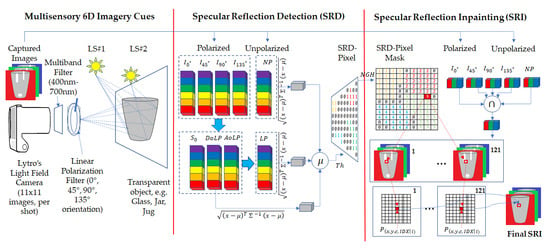
4. Proposed Two-fold SRDI Framework

In this section, the proposed two-fold SRDI framework based on the distinctive features of MSPLFI cues is discussed and presented in Figure 6. Firstly, a 6D dataset of different transparent objects is captured, and then Reed-Xiaoli (RX) detector [53] is applied to obtain the actual specular reflection of an object through predicting changes among multiband. Secondly, a pixel neighborhood-based inpainting method for suppressing this reflection is proposed.

4.1. Specular Reflection Detection (SRD)

The proposed system detects specular reflected pixels in transparent objects through predictions of multiband changes. Firstly, a raw lenslet (.LFR) image is decoded into a 4D ($s,t,u,v$) LF one, where ($s,t$) denotes the image’s position in the hyperplane and ($u,v$) its spatial region. The MSPLF imagery was captured by the Lytro Illum camera, which can capture 15 × 15 sub-apertures per shot. However, due to the main lens of the camera being circular, vignetting occurs at its edge. Hence, only the inner 11 × 11 sub-apertures are retained. It could be argued that few more sub-apertures at the top, the bottom, the left, and the right could be as good—if not better—than the corner sub-apertures kept in the 11 × 11 array, but excluding them keeps them in a square array for simplicity. As our main purpose is to detect and suppress specularity in a transparent object, we maximize an object’s area with a minimum surrounding background. In order to compute the specular reflections in unpolarized images, we convert all the multiband unpolarized 4D LF ones into their corresponding grayscale ones. For each sub-aperture index, we store the individual band images in a column vector, with their mean ($\mu$) and covariance ($\Sigma$) calculated for the Mahalanobis distance as

$$\sqrt{{\left(x-\mu \right)}^T{\Sigma }^{-1}\left(x-\mu \right)},$$

(5)

The 2D distance matrix represents the changes among the multiband images per sub-aperture index, which is also observed as specular reflection. We also predict the maximum specularity in unpolarized 4D images. In order to draw specular reflections in polarized images, we firstly calculate the Stokes parameters ($S_0$−$S_2$) [54], which describe the linear polarization characteristics using a three-element vector ($S$), as shown in Equation (6), where $S_0$ represents the total intensity of light, $S_1$ the difference between the horizontal and vertical polarizations, and $S_2$ the difference between the linear +45° and –45° ones. The $I_{0^0}$, $I_{{45}^0}$, $I_{{90}^0}$, and $I_{{135}^0}$ are the different input images for the system at polarized angles of $0^0,{45}^0,{90}^0,$ and ${135}^0$, respectively.

$$S=\left[\begin{array}{c}{S}_0\\ S_1\\ S_2\end{array}\right]=\left[\begin{array}{c}{I}_{0^0}+I_{{90}^0}\\ I_{0^0}-I_{{90}^0}\\ I_{{45}^0}-I_{{135}^0}\end{array}\right],$$

(6)

The degree of linear polarization ($DoLP$) is a measure of the proportion of the linear polarized light relative to the light’s total intensity, and the angle of linear polarization ($AoLP$) is the orientation of the major axis of the polarization ellipse, which represents the polarizing angle where the intensity should be the strongest. They are derived from the Stokes vector according to Equations (7) and (8), respectively. To calculate the linear polarized image, firstly, the polarimetric components are concatenated, as shown in Equation (9). Then, a concatenated image is generated in the hue, saturation, value (HSV) color space and converted to the RGB color space, as in Equation (10), where $LP$ stands for linear polarization.

$$DoLP=\frac{I_{pol}}{I_{tot}}=\frac{\sqrt{S_1^2+S_2^2}}{S_0},$$

(7)

$$AoLP=\frac{1}{2}ta{n}^{-1}\left(\frac{S_2}{S_1}\right),$$

(8)

$$hsv=\left(\left(AoLP+\pi /2\right)/\pi \right){}^{⏜}\left(DoLP\times 2\right){}^{⏜}{S}_0,$$

(9)

$$LP=RGB\left(hsv\right),$$

(10)

For each sub-aperture index of $DoLP$ and $LP$, we store individual band images in a separate column vector. Then, a similar procedure (unpolarized specular detection) is followed to calculate the maximum specularity in the LP and the DoLP 4D imagery. The average of three specularities ($RX-NP,RX-LP,RX-DoLP$) shows the overall predicted specularity in an object of MSPLFI, with a threshold (Otsu’s method and in the range (0–1)) applied to obtain the SRD pixels in binary form. The complete process for detecting specular pixels in a transparent object is described in Algorithm 1.

Algorithm 1. SRD in Transparent Object

Input: MSPLFI Object Dataset

Output: SRD Pixel in Binary

1: for all lenslet (.LFR) image do

2:  Decode raw lenslet (.LFR) multiband polarized and unpolarized images into 4D ($\mathit{s},\mathit{t},\mathit{u},\mathit{v}$) LF images

3:  Remove and clip unwanted images and pixels

4: end for

5: for all sub-aperture image do

6:  for all multiband do

7:    Calculate $\mathit{D}\mathit{o}\mathit{L}\mathit{P},\mathit{L}\mathit{P}$ as in Equations (7)–(10)

8:    if type ($\mathit{L}\left(\mathit{u},\mathit{v},\mathit{s},\mathit{t},\mathit{\lambda },\mathit{\rho }\right)$ = “unpolarized” then

9:     Convert multiband image into corresponding grayscale       Store multiband grayscale image as column vector

10:    else if type ($\mathit{L}\left(\mathit{u},\mathit{v},\mathit{s},\mathit{t},\mathit{\lambda },\mathit{\rho }\right)$ = “polarized” then

11:      Store multiband image as column vector

12:    end if

13:  end for

14:  Calculate mean ($\mathit{\mu }$) and covariance ($\mathbf{\Sigma }$) per sub-aperture index of LF

15:  Calculate Mahalanobis distance as in Equation (5)

16:  Reshape distance vector as 2D image which represents SRD per sub-aperture image

17: end for

18: Calculate maximum changes/specularities observed in all sub-aperture indexes for object type “$\mathit{R}\mathit{X}-\mathit{N}\mathit{P}$”

19: repeat steps 5–18 for object type = “$\mathit{R}\mathit{X}-\mathit{D}\mathit{o}\mathit{L}\mathit{P}$” and object type= “$\mathit{R}\mathit{X}-\mathit{L}\mathit{P}$”

20: Calculate mean ($\mathit{\mu }$) specularity of object type: $\mathit{R}\mathit{X}-\mathit{N}\mathit{P}$, $\mathit{R}\mathit{X}-\mathit{D}\mathit{o}\mathit{L}\mathit{P}$ and $\mathit{R}\mathit{X}-\mathit{L}\mathit{P}$

21: Apply threshold ($\mathit{\tau }$) to binarize SRD pixels

4.2. Specular Reflection Inpainting (SRI)

In this research, the SRD pixels are suppressed through analyzing the distances among four connected neighboring pixels. Firstly, four different regions in an image are identified, as shown in Figure 7. Algorithm 1 predicts region A as an SRD pixel but, for better inpainting quality, both regions A and B are considered specular reflected pixels. It is to be noted that region B contains the pixel patterns (color channels) that are the immediate neighbors of region A. Then, all the connected regions are identified and labeled for the task of inpainting. The complete process for inpainting the detected specular pixels in transparent object is described in Algorithm 2.

Algorithm 2. SRI in Transparent Object

Input: MSPLFI Object Dataset, SRD-PM

Output: SRD Pixel Inpainting in RGB

1: Strengthen SRD-PM (output from Algorithm 1) by labeling all neighboring pixels as SRD ones

2: Compute connected components and label them

3: Calculate baseline image per sub-aperture index by taking minimum pixel intensities of both polarized and unpolarized images in RGB channels

4: for all common sub-aperture images do

5:  for all labels do

6:    for all pixel patterns (${\mathit{P}}_{(\mathit{x},\mathit{y},\mathit{c}|\mathit{i})}$) in SRD-PM do

7:      if labels (SRD-PMs) exist then

8:        Compute distances (${\mathit{d}}_{(\mathit{j},\mathit{k}|\mathit{x},\mathit{y})}$) among 4-connected neighbors not in SRD-PM in each channel, as in Equation (11), and store them in 2D-matrix ($\mathit{d}{\mathit{M}}_{\left(\mathit{n}\mathit{r}\mathit{o}\mathit{w},\mathit{n}\mathit{c}\mathit{o}\mathit{l}\right)}$), as in Equation (12)

9:        Winning pixel pattern is index ($\mathit{I}\mathit{D}\mathit{X}$) of pixel pattern corresponding to column-wise minimum sum of $\mathit{d}{\mathit{M}}_{\left(\mathit{n}\mathit{r}\mathit{o}\mathit{w},\mathit{n}\mathit{c}\mathit{o}\mathit{l}\right)}$, as in Equations (13) and (14) for inpainting of specular reflections

10:      end if

11:    end for

12:  end for

13: end for

14: repeat steps 4 to 13 to calculate maximum specular reflection in suppressed image of transparent object from already suppressed sub-apertures

A baseline image per sub-aperture index is computed by taking the minimum pixel intensities in both polarized and unpolarized RGB channels. The aim is to suppress the specular reflected areas in the image, with the distance between two pixel-patterns calculated by

$$d_{(j,k|x,y)}=\sqrt{{\sum }_{c=R,G,B}{\left(P_{(x,y,c,j|i)}-P_{(x,y,c,k|i)}\right)}^2},$$

(11)

where $P_{(x,y,c,j|i)}$ and $P_{(x,y,c,k|i)}$ are the two four-connected neighbors of the pixel pattern ($P_{(x,y,c|i)}$) in sub-aperture index $i$ and $d_{(j,k|x,y)}$ the distance between the two pixel patterns corresponding to $P_{(x,y,c|i)}$ in sub-aperture index $i$. A 2D matrix [55] of the distances among the pixel patterns is calculated by Equation (12). The pattern corresponding to the lowest column-wise sum of the distances is selected as the winning one ($P_{(x,y,c,IDX|i)}$) for the task of SRI in Equations (13) and (14).

$$d{M}_{\left(nrow,ncol\right)}=\left(\begin{array}{ccc}{d}_{(j-4,k-4|x,y)}& \dots & d_{(j+4,k-4|x,y)}\\ ⋮& d_{(j,k|x,y)}& ⋮\\ d_{(j-4,k+4|x,y)}& \dots & d_{(j+4,k+4|x,y)}\end{array}\right)$$

(12)

$$IDX=\begin{array}{c}argmin\\ k\end{array}\sum d{M}_{\left(nrow,k\right)}$$

(13)

$$P_{(x,y,c|i)}=P_{(x,y,c,IDX|i)}$$

(14)

5. Experimental Results

In this section, performance evaluations and comparisons of the proposed two-fold SRDI and other approaches using different metrics for specular pixel detection and inpainting are discussed. Additionally, analyses of their computational times are conducted.

5.1. Selection of Performance Evaluation Metric

Both SRD and SRI are evaluated by commonly used statistical evaluation metrics for quantifying detection accuracy and inpainting quality.

5.1.1. Selection of SRD Metric

The SRD method is evaluated at the pixel level of a binarized scene in which the pixels related to the specular and the diffuse reflections are white and black, respectively. Its performance can be divided into four pixel-wise classification results: true positive ($T_p$), which means a correctly detected diffuse pixel; false positive ($F_p$), that is, a specular reflected pixel incorrectly detected as a diffuse reflected one; true negative ($T_n$), which indicates a correctly detected pixel with specularity; and false negative ($F_n$), that is, a diffuse reflected pixel incorrectly detected as a specular reflected one. The binary classification metrics used are precision, recall or sensitivity, F1-score, specificity, geometric-mean (G-mean), and accuracy. Precision is the number of diffuse reflected pixels detected that are actually diffuse reflected ones, while recall is the number of diffuse reflected pixels detected from the actual diffuse reflected ones (recall and sensitivity are similar). The F1-score (a boundary F1 measure) is the harmonic mean of precision and recall values, which measures how closely the predicted boundary of an object matches its ground-truth and is an overall indicator of the performance of binary segmentation. Specificity (a $T_n$ fraction) is the proportion of actual negatives predicted as negatives, sensitivity (a $T_p$ fraction) the proportion of actual positives predicted as positives, G-mean the root of the product of specificity and sensitivity, and accuracy the proportion of true results obtained, either $T_n$ or $T_p$. The mathematical evaluation measures of the aforementioned metrics are shown in Equations (15) to (20) [17,56].

$$Precision\left(PR\right)=\frac{T_p}{T_p+F_p},$$

(15)

$$Recall\left(RC\right)orSensitivity\left(SN\right)=\frac{T_p}{T_p+F_n},$$

(16)

$$F1-Score\left(F1S\right)=2\times \frac{Precision\times Recall}{Precision+Recall},$$

(17)

$$Specificity\left(SP\right)=\frac{T_n}{T_n+F_p},$$

(18)

$$Geometric-Mean\left(GM\right)=\sqrt{Specificity\times Sensitivity},$$

(19)

$$Accuracy\left(AC\right)=\frac{T_p+T_n}{T_p+F_n+T_n+F_p},$$

(20)

5.1.2. Selection of Inpainting Quality Metric

Currently, the quality of a fused image can be quantitively evaluated using the metrics [57] structural similarity index (SSIM), peak signal-to-noise ratio (PSNR), mean squared error (IMMSE), and mean absolute deviation (MAD). The SSIM is an assessment index of the image quality based on computations of luminance, contrast, and structural components of the reference and the reconstructed images, with the overall index a multiplicative combination of these three components. The PSNR block computes the PSNR between the reference and the suppressed images in decibels (dB), with higher values of SSIM and PSNR indicating better quality of the reconstructed or the suppressed image. The IMMSE computes the average squared error between the reference and the reconstructed images, while MAD indicates the sum of the absolute differences between the pixel values of these images divided by the total number of pixels, which is used to measure the standard error of the reconstructed image. Lower values of IMMSE and MAD indicate better quality of the reconstructed image. Considering two images ($x$ and $y$), the aforementioned mathematical evaluation metrics are shown in Equations (21) to (24).

$$SSIM\left(x,y\right)=\left[l{\left(x,y\right)}^{\alpha }\right]·\left[c{\left(x,y\right)}^{\beta }\right]·\left[s{\left(x,y\right)}^{\gamma }\right],$$

(21)

where,

$$l\left(x,y\right)=\frac{2{\mu }_x{\mu }_y+C_1}{{\mu }_x^2+{\mu }_y^2+C_1}c\left(x,y\right)=\frac{2{\sigma }_x{\sigma }_y+C_2}{{\sigma }_x^2+{\sigma }_y^2+C_2}s\left(x,y\right)=\frac{{\sigma }_{xy}+C_3}{{\sigma }_x{\sigma }_y+C_3}$$

where ${\mu }_x$, ${\mu }_y$, ${\sigma }_x$, ${\sigma }_y$ and ${\sigma }_{xy}$ are local means, standard deviations, and cross-covariances of images $x$ and $y$.

$$PSNR\left(x,y\right)=10.lo{g}_{10}\left(\frac{MA{X}_I^2}{IMMSE\left(x,y\right)}\right),$$

(22)

where $MAX$ denotes the range of the image ($xory$) datatype

$$IMMSE\left(x,y\right)=\frac{1}{n}{\sum }_{i=1}^n{\left(x_i-y_i\right)}^2,$$

(23)

$$MAD\left(x,y\right)=\frac{1}{n}{\sum }_{i=1}^n\left|\left(x_i-y_i\right)\right|,$$

(24)

5.2. Generation of Ground Truth

To evaluate the performance of the proposed two-fold SRDI, we generate two different ground truths for each object, as shown in Figure 8. The SRD and the SRI ones are created manually by an expert, with the maximum possible specular reflected area in the MSPLFI object dataset covered. Figure 8 shows the two-way SRD ground truth generation, where a pixel with an intensity above a threshold (Otsu’s method and in the range (0–1)) level is considered a specular reflected pixel. The final column in Figure 13 presents the objects’ SRD binary ground truths, with black and white pixels indicating their diffuse and specular reflected pixels, respectively. The final column in Figure 18 shows the objects’ SRI ground truths. Due to the real scene in the MSPLFI object dataset, some pixels in an object may exhibit amounts of both specular and diffuse reflections but, to measure the performance in terms of quantity and enable further comparisons, each pixel is classified manually as either specular or diffuse reflected, and the ground truth is re-named as the quasi-ground truth.

5.3. Performance Evaluation of SRD

5.3.1. Analysis of SRD Rate

Figure 9 shows the SRD rates in terms of the SRD metrics of precision, recall, F1-score, G-mean, and accuracy for nine sample objects both separately (Figure 9) and together for all objects (O#1–O#18) (Figure 10) using the proposed method. For each object, a total of 121 sub-aperture images are used to measure its specularity and box plots to statistically analyze our experiments. Figure 9 exhibits the SRD metric values obtained for nine sample objects separately. Remaining objects are presented in Appendix A (Figure A1). Accuracy has a higher median value than the F1-score and the G-mean for all the objects, with O#9 and O#3 having superior median values of 0.804, 0.832, and 0.996, and 0.874, 0.882, and 0.991 for F1-score, G-mean, and accuracy, respectively, compared with those of the other objects.

Similarly, Figure 10 shows the combined SRD rates for 121 sub-aperture + 1 maximum images × 18 objects = 2196 images. Accuracy has a better overall median and 75th percentile values for all the objects combined (0.981 and 0.992, respectively) compared to the F1-score (0.643 and 0.770, respectively) and the G-mean (0.656 and 0.752, respectively).

5.3.2. Comparison of SRD Rates of Proposed Method and Those in Literature

It is worth mentioning that the performances of the existing SRD methods considered are not exactly comparable, as each reports its accuracy for a specific image set using different contexts. Moreover, the accuracy values obtained from them and the color-mapping techniques used for segmentation may vary.

In

Table 1. Performance evaluation of different methods in terms of various SRD metrics for 18 objects (O#1–O#18) in MSPLFI object dataset and overall means (all sub-aperture images in 4D LF).

Methods	Metrics	Object Index (Maximum SRD)																		Overall Mean (SA)
		O#1	O#2	O#3	O#4	O#5	O#6	O#7	O#8	O#9	O#10	O#11	O#12	O#13	O#14	O#15	O#16	O#17	O#18
Ak. [40]	Precision	0.178	0.348	0.686	0.445	0.600	0.354	0.460	0.382	0.655	0.519	0.240	0.311	0.336	0.124	0.522	0.542	0.504	0.123	0.362 ± 0.24
	Recall	0.628	0.629	0.662	0.427	0.514	0.345	0.426	0.417	0.771	0.536	0.598	0.866	0.658	0.622	0.466	0.727	0.328	0.747	0.512 ± 0.14
	F1-Score	0.277	0.448	0.673	0.436	0.554	0.350	0.443	0.398	0.708	0.528	0.342	0.457	0.445	0.207	0.493	0.621	0.398	0.211	0.377 ± 0.16
	G-Mean	0.769	0.781	0.810	0.644	0.710	0.578	0.644	0.634	0.874	0.722	0.749	0.917	0.795	0.754	0.676	0.835	0.567	0.834	0.689 ± 0.10
	Accuracy	0.935	0.962	0.981	0.943	0.957	0.939	0.946	0.939	0.986	0.948	0.928	0.970	0.951	0.910	0.960	0.944	0.940	0.929	0.926 ± 0.05
Sn. [35]	Precision	0.220	0.610	0.759	0.509	0.613	0.437	0.527	0.477	0.602	0.579	0.462	0.447	0.574	0.388	0.590	0.642	0.622	0.505	0.655 ± 0.15
	Recall	0.667	0.590	0.639	0.392	0.493	0.301	0.411	0.335	0.831	0.546	0.513	0.848	0.457	0.474	0.476	0.647	0.275	0.599	0.483 ± 0.15
	F1-Score	0.330	0.600	0.694	0.443	0.546	0.357	0.462	0.393	0.698	0.562	0.486	0.586	0.509	0.426	0.527	0.644	0.381	0.548	0.527 ± 0.13
	G-Mean	0.797	0.764	0.797	0.620	0.696	0.543	0.635	0.573	0.906	0.730	0.709	0.913	0.672	0.683	0.685	0.794	0.522	0.771	0.681 ± 0.11
	Accuracy	0.946	0.981	0.983	0.949	0.958	0.948	0.952	0.950	0.984	0.954	0.966	0.983	0.974	0.976	0.964	0.955	0.946	0.988	0.969 ± 0.01
Yn. [1]	Precision	0.220	0.396	0.603	0.402	0.476	0.269	0.382	0.364	0.595	0.438	0.274	0.224	0.288	0.166	0.416	0.494	0.448	0.156	0.433 ± 0.19
	Recall	0.817	0.638	0.673	0.457	0.562	0.430	0.442	0.475	0.831	0.571	0.630	0.884	0.671	0.652	0.484	0.758	0.383	0.754	0.529 ± 0.16
	F1-Score	0.346	0.488	0.636	0.428	0.515	0.331	0.410	0.413	0.694	0.496	0.382	0.358	0.403	0.265	0.447	0.598	0.413	0.258	0.446 ± 0.14
	G-Mean	0.877	0.789	0.815	0.664	0.737	0.636	0.652	0.675	0.906	0.739	0.772	0.919	0.798	0.782	0.686	0.848	0.609	0.845	0.707 ± 0.11
	Accuracy	0.939	0.968	0.977	0.937	0.946	0.917	0.936	0.935	0.984	0.937	0.936	0.954	0.941	0.931	0.950	0.936	0.934	0.945	0.953 ± 0.02
Ym. [37]	Precision	0.199	0.409	0.657	0.435	0.531	0.282	0.302	0.357	0.631	0.406	0.243	0.222	0.296	0.122	0.403	0.364	0.513	0.143	0.307 ± 0.23
	Recall	0.645	0.634	0.665	0.435	0.547	0.384	0.456	0.458	0.778	0.565	0.646	0.875	0.680	0.647	0.492	0.791	0.328	0.755	0.559 ± 0.15
	F1-Score	0.304	0.497	0.661	0.435	0.539	0.325	0.363	0.401	0.697	0.472	0.353	0.355	0.412	0.205	0.443	0.499	0.400	0.240	0.346 ± 0.17
	G-Mean	0.782	0.787	0.811	0.649	0.730	0.604	0.656	0.663	0.877	0.734	0.777	0.914	0.804	0.767	0.691	0.847	0.567	0.843	0.709 ± 0.10
	Accuracy	0.941	0.969	0.980	0.942	0.952	0.924	0.920	0.934	0.985	0.932	0.925	0.954	0.942	0.905	0.948	0.900	0.940	0.939	0.908 ± 0.06
Ar. [41]	Precision	0.189	0.520	0.463	0.471	0.529	0.258	0.436	0.383	0.410	0.468	0.308	0.191	0.287	0.178	0.366	0.496	0.413	0.255	0.561 ± 0.12
	Recall	0.594	0.587	0.668	0.394	0.391	0.351	0.422	0.449	0.763	0.526	0.609	0.877	0.353	0.281	0.467	0.727	0.371	0.447	0.434 ± 0.16
	F1-Score	0.287	0.552	0.547	0.429	0.450	0.298	0.428	0.414	0.534	0.495	0.409	0.314	0.317	0.218	0.410	0.590	0.391	0.325	0.466 ± 0.10
	G-Mean	0.750	0.761	0.808	0.620	0.619	0.577	0.640	0.658	0.863	0.713	0.763	0.910	0.586	0.524	0.671	0.831	0.598	0.663	0.644 ± 0.12
	Accuracy	0.941	0.977	0.967	0.946	0.951	0.921	0.943	0.939	0.971	0.942	0.945	0.944	0.955	0.962	0.944	0.936	0.930	0.976	0.966 ± 0.01
St. [42]	Precision	0.461	0.679	0.680	0.597	0.692	0.344	0.609	0.392	0.586	0.616	0.340	0.237	0.491	0.360	0.421	0.631	0.487	0.193	0.702 ± 0.12
	Recall	0.592	0.535	0.637	0.357	0.502	0.321	0.400	0.381	0.771	0.462	0.558	0.876	0.457	0.394	0.495	0.567	0.315	0.724	0.422 ± 0.15
	F1-Score	0.518	0.598	0.658	0.447	0.582	0.332	0.483	0.387	0.666	0.528	0.423	0.373	0.473	0.376	0.455	0.597	0.383	0.305	0.507 ± 0.11
	G-Mean	0.764	0.729	0.795	0.593	0.704	0.558	0.628	0.608	0.873	0.674	0.734	0.916	0.671	0.624	0.693	0.744	0.555	0.834	0.637 ± 0.12
	Accuracy	0.978	0.983	0.980	0.954	0.963	0.939	0.957	0.942	0.983	0.955	0.952	0.957	0.970	0.975	0.950	0.952	0.938	0.958	0.971 ± 0.01
Ms. [43]	Precision	0.646	0.878	0.914	0.876	0.765	0.592	0.754	0.585	0.847	0.702	0.557	0.557	0.556	0.348	0.692	0.657	0.729	0.660	0.868 ± 0.09
	Recall	0.580	0.367	0.502	0.248	0.485	0.212	0.393	0.307	0.568	0.445	0.507	0.831	0.489	0.572	0.366	0.627	0.240	0.338	0.283 ± 0.11
	F1-Score	0.611	0.518	0.648	0.387	0.593	0.312	0.517	0.403	0.680	0.545	0.530	0.667	0.520	0.433	0.479	0.642	0.361	0.447	0.412 ± 0.13
	G-Mean	0.759	0.606	0.708	0.498	0.694	0.459	0.625	0.551	0.753	0.664	0.707	0.907	0.695	0.748	0.603	0.783	0.489	0.581	0.520 ± 0.11
	Accuracy	0.985	0.983	0.984	0.959	0.966	0.956	0.963	0.956	0.988	0.960	0.972	0.988	0.973	0.971	0.967	0.956	0.949	0.989	0.971 ± 0.01
Proposed	Precision	0.630	0.666	0.728	0.622	0.668	0.643	0.798	0.563	0.756	0.678	0.485	0.624	0.470	0.422	0.665	0.658	0.719	0.614	0.776 ± 0.10
	Recall	0.630	0.585	0.737	0.798	0.946	0.281	0.767	0.452	0.808	0.613	0.526	0.720	0.554	0.718	0.553	0.784	0.320	0.578	0.444 ± 0.15
	F1-Score	0.630	0.623	0.732	0.699	0.783	0.391	0.782	0.501	0.781	0.644	0.504	0.668	0.509	0.531	0.604	0.715	0.442	0.596	0.546 ± 0.13
	G-Mean	0.791	0.762	0.855	0.881	0.960	0.528	0.871	0.666	0.896	0.777	0.718	0.846	0.737	0.839	0.739	0.873	0.563	0.759	0.654 ± 0.11
	Accuracy	0.985	0.983	0.984	0.965	0.973	0.958	0.978	0.957	0.990	0.963	0.967	0.990	0.968	0.976	0.970	0.961	0.951	0.990	0.974 ± 0.01

, the performances of SRD in terms of different evaluation metrics for the proposed and other methods are compared for the 18 individual objects. For visualization purposes, short forms of the authors’ names are written in the first column, that is, Ak., Sn., Yn., Ym., Ar., St., and Ms. refer to Akashi, Shen, Yang, Yamamoto, Arnold, Saint, and Meslouhi, respectively. The SRD metric values in the object index columns correspond to the maiden specular image among the sub-aperture ones. The final column (overall mean ?SA)) corresponds to the mean ± SD values of the 121 sub-aperture + 1 maximum images × 18 objects = 2196 images together.

As can be seen, the overall mean SRD different metric values are higher for the proposed method than the studies discussed in this paper, as shown in the final column in Table 1. Additionally, considering all the sub-aperture images of the 18 distinct objects, mean F1-score, G-mean, and accuracy values for the proposed method are 0.546 ± 0.13, 0.654 ± 0.11 and 0.974 ± 0.01, respectively. In Figure 11, the SRD metric values for the 18 individual objects (O#1–O#18) and their maximum specular reflections obtained from different methods are compared. As can be seen, the proposed method achieves superior median values for the F1-score, G-mean and accuracy of 0.662, 0.816 and 0.971, respectively.

In Figure 12, the SRD metric values for 121 sub-aperture + 1 maximum images × 18 objects = 2196 images with their specular reflections obtained by different methods are presented. As can be seen, the proposed method has superior median values for F1-score, G-mean, and accuracy of 0.643, 0.676, and 0.981, respectively, to those of the others.

5.3.3. Visualization of SRD Rates of Different Methods

In Figure 13, the SRD accuracies obtained by different methods for the maximum specular reflected images of sample objects in the MSPLFI object dataset are presented. As can be seen, the proposed approach reports fewer SRD errors than the others. Remaining objects are presented in Appendix A (Figure A2).

5.4. Performance Evaluation of SRI

5.4.1. Analysis of SRI Quality

The SRI qualities in terms of the normalized SRI metrics SSIM, PSNR, IMMSE, and MAD for the nine sample objects using the proposed method are presented separately in Figure 14 and then together for all objects (O#1–O#18) in Figure 15. For each object, a total of 121 sub-aperture + 1 maximum images are considered to measure its SRI and box plots used to statistically analyze our experiments. It is to be noted that a suppressed image with high SSIM and PSNR values and low IMMSE and MAD ones is close to the quasi-ground truth. Figure 14 shows that the SSIM has a higher median value than the PSNR but the IMMSE a lower one than the MAD for all the objects while object O#1 has superior median values of 0.966, 0.820, 0.038, and 0.131 for SSIM, PSNR, IMMSE, and MAD, respectively, to those of the other objects. Remaining objects are presented in Appendix B (Figure A3). Similarly, Figure 15 shows the normalized SRI qualities of (121 Sub-aperture + 1 maximum) × 18 Objects = 2196 images together. The SSIM has better overall median and 75^th percentile values for all the objects combined (0.966 and 0.980, respectively) than the PSNR (0.735 and 0.778, respectively) and the IMMSE better overall median and 75th percentile values for all the objects (0.073 and 0.118, respectively) than the MAD (0.226 and 0.273, respectively).

5.4.2. Comparison of SRI Rates of Proposed Method and Those in Literature

It is worth mentioning that the performances of the existing SRI methods are not exactly comparable, as each reports its accuracy for a specific image set in a different context. Additionally, the quality obtained by the methods and the color-mapping techniques used for inpainting may vary.

In

Table 2. Performance evaluations of different methods using different SRI metrics for 18 objects (O#1–O#18) and overall mean (all sub-aperture images in 4D LF) in MSPLFI object dataset.

Methods	Metrics	Object Index (Maximum SRI)																		Overall Mean (SA)
		O#1	O#2	O#3	O#4	O#5	O#6	O#7	O#8	O#9	O#10	O#11	O#12	O#13	O#14	O#15	O#16	O#17	O#18
Ar. [41]	SSIM	0.942	0.967	0.966	0.965	0.940	0.961	0.940	0.959	0.965	0.929	0.940	0.946	0.968	0.958	0.925	0.943	0.963	0.955	0.941 ± 0.02
	PSNR	21.25	20.42	21.26	20.96	19.99	20.95	19.22	20.25	20.74	19.03	18.33	18.53	20.83	18.58	18.42	19.56	20.98	19.65	19.80 ± 0.99
	IMMSE	487.6	590.1	486.2	520.9	651.4	522.7	778.0	613.9	548.7	813.4	954.8	911.5	537.6	901.9	935.8	720.2	519.3	705.4	698.9 ± 162
	MAD	12.53	16.20	16.26	15.26	13.49	14.89	19.94	15.12	15.79	18.51	18.87	19.80	12.74	17.97	19.63	18.27	13.55	15.52	16.46 ± 2.36
Yg. [51]	SSIM	0.887	0.956	0.943	0.951	0.926	0.951	0.910	0.952	0.954	0.922	0.944	0.943	0.960	0.948	0.911	0.915	0.958	0.957	0.926 ± 0.02
	PSNR	18.31	19.74	20.16	21.42	18.44	20.53	19.29	20.12	20.43	18.72	18.95	19.06	21.36	18.98	17.68	18.78	22.01	20.45	19.53 ± 1.14
	IMMSE	958.6	690.6	626.5	468.5	931.3	574.9	766.7	632.8	589.2	872.9	828.4	807.7	475.5	822.3	1110	861.8	408.9	586.0	749.8 ± 190
	MAD	18.05	16.36	17.15	13.68	16.01	14.88	19.06	14.88	15.52	18.68	17.16	18.36	11.26	16.34	20.98	19.36	11.58	13.77	16.48 ± 2.58
Cr. [52]	SSIM	0.956	0.968	0.964	0.948	0.924	0.963	0.922	0.961	0.965	0.927	0.944	0.947	0.962	0.956	0.925	0.940	0.962	0.955	0.935 ± 0.02
	PSNR	22.50	20.60	21.40	20.48	19.52	21.31	19.06	20.64	20.84	19.16	18.68	18.90	20.97	18.63	18.60	19.65	21.23	19.74	19.89 ± 1.04
	IMMSE	365.8	566.9	471.8	582.8	726.3	480.6	807.4	561.7	536.1	789.5	881.6	838.4	519.9	891.1	897.0	704.5	489.6	690.5	685.5 ± 161
	MAD	11.41	15.90	16.09	16.04	14.36	14.31	20.33	14.56	15.69	18.23	18.12	19.08	12.45	17.78	19.25	18.03	13.24	15.34	16.27 ± 2.36
St. [42]	SSIM	0.956	0.968	0.967	0.966	0.945	0.967	0.943	0.966	0.966	0.933	0.948	0.952	0.970	0.957	0.929	0.939	0.967	0.957	0.941 ± 0.02
	PSNR	22.49	20.59	21.41	21.11	20.07	21.30	19.54	20.61	20.88	19.23	18.60	18.90	21.10	18.66	18.54	19.83	21.42	19.70	20.01 ± 1.05
	IMMSE	366.4	567.2	469.7	504.1	639.7	482.0	722.3	565.5	531.5	776.6	896.9	837.2	505.1	886.4	910.4	676.7	469.1	696.4	667.6 ± 162
	MAD	11.54	15.89	16.06	14.91	13.39	14.35	19.04	14.68	15.59	18.13	18.32	19.00	12.29	17.73	19.41	17.48	12.99	15.40	16.04 ± 2.31
Ak. [40]	SSIM	0.918	0.979	0.938	0.941	0.913	0.928	0.900	0.929	0.943	0.899	0.907	0.912	0.942	0.933	0.889	0.914	0.931	0.928	0.899 ± 0.03
	PSNR	19.36	24.30	18.49	18.93	17.00	17.89	16.82	17.17	18.41	16.27	15.49	16.00	17.80	16.09	15.84	16.48	17.89	17.29	17.08 ± 1.12
	IMMSE	753.7	241.5	921.2	831.6	1296	1057	1351	1248	936.8	1536	1838	1631	1080	1598	1694	1464	1057	1215	1315 ± 334
	MAD	16.45	6.36	21.45	18.77	19.43	21.19	25.70	21.51	19.96	25.54	26.17	26.52	17.80	23.90	26.31	25.87	19.20	20.28	22.23 ± 3.24
Sn. [35]	SSIM	0.936	0.961	0.957	0.952	0.923	0.959	0.922	0.956	0.951	0.917	0.937	0.941	0.964	0.952	0.915	0.934	0.961	0.954	0.929 ± 0.02
	PSNR	19.32	19.99	20.78	19.94	18.23	20.78	18.17	19.97	19.13	17.73	18.09	18.42	20.41	18.23	17.80	19.09	21.01	19.57	19.06 ± 1.05
	IMMSE	760.9	652.2	543.6	659.6	976.7	543.1	992.1	654.8	795.4	1101	1009	934.8	591.4	976.5	1079	802.5	515.3	717.4	830.7 ± 197
	MAD	14.60	16.80	16.93	16.37	15.95	15.05	21.35	15.56	17.49	20.55	19.31	20.04	13.20	18.55	20.66	18.99	13.48	15.61	17.43 ± 2.43
Ym. [37]	SSIM	0.906	0.952	0.945	0.949	0.917	0.934	0.897	0.933	0.950	0.894	0.911	0.912	0.938	0.920	0.890	0.880	0.944	0.938	0.902 ± 0.03
	PSNR	18.37	18.83	19.11	19.46	17.72	18.69	16.37	17.72	19.11	16.01	15.97	16.23	17.87	15.57	15.86	14.84	19.34	18.20	17.27 ± 1.44
	IMMSE	946.5	852.3	798.1	737.0	1100	879.5	1500	1098	797.6	1631	1643	1550	1061	1804	1686	2134	756.5	985.2	1289 ± 439
	MAD	17.89	18.57	19.20	17.36	17.35	18.92	25.95	19.38	17.99	25.54	23.94	25.24	16.79	24.04	25.59	29.90	15.81	18.03	21.27 ± 4.11
Proposed	SSIM	0.992	0.990	0.989	0.972	0.941	0.984	0.961	0.973	0.991	0.947	0.964	0.977	0.978	0.982	0.950	0.953	0.983	0.983	0.956 ± 0.02
	PSNR	33.43	26.16	29.24	22.79	22.26	29.85	25.60	25.06	29.27	23.84	22.76	24.62	26.52	24.91	21.76	22.37	27.64	25.36	24.51 ± 2.11
	IMMSE	29.54	157.4	77.50	341.9	386.7	67.34	179.2	202.9	76.95	268.6	344.8	224.2	145.1	209.9	433.9	376.7	112.1	189.2	257.6 ± 119
	MAD	1.172	7.903	5.205	7.680	8.536	4.529	8.723	8.277	4.959	10.07	11.07	8.888	5.257	7.880	13.26	12.97	5.545	7.665	8.427 ± 2.51

SSIM: structural similarity index; PSNR: peak signal-to-noise ratio; IMMSE: mean squared error; MAD: mean absolute deviation.

, the performances of SRI in the proposed and other methods for the 18 individual objects are compared using different evaluation metrics. For visualization, short forms of the authors’ names written in the first column as Ar., Yg., Cr., St., Ak., Sn., and Ym. refer to Arnold, Yang, Criminisi, Saint, Akashi, Shen, and Yamamoto, respectively. The SRI metric values in the object index columns correspond to the maiden image of the 121 sub-aperture specular reflected suppressed ones. The final column (overall mean (SA)) corresponds to the mean ± SD values of the 121 sub-aperture + 1 maximum images × 18 objects = 2196 images together. As can be seen, the SRI metric values are significantly better for the proposed method than for the others considered, as shown in the final column in Table 2. For all the sub-aperture images of the 18 distinct objects, the mean SSIM, PSNR, IMMSE, and MAD values obtained from the proposed method are 0.956 ± 0.02, 24.51 ± 2.11, 257.6 ± 119, and 8.427 ± 2.51, respectively.

In Figure 16, comparisons of the SRI metric values of individual methods in terms of SSIM, PSNR, IMMSE, and MAD of 18 individual objects (O#1–O#18) with their maiden specular inpainting is presented. It can be seen that the proposed method has superior median values for SSIM and PSNR of 0.985 and 0.754 and the lowest median values for IMMSE and MAD of 0.063 and 0.217, respectively.

Figure 17 shows the SRI metric values of individual methods in terms of SSIM, PSNR, IMMSE, and MAD of 121 sub-aperture + 1 maiden images × 18 objects = 2196 images. As can be seen, the proposed method has superior median values for SSIM and PSNR of 0.966 and 0.735, respectively, and the lowest median values for IMMSE and MAD of 0.073 and 0.226, respectively, compared with those of the other methods.

5.4.3. Visualization of SRI Quality Assessment

Figure 18 presents the SRI qualities obtained by different methods for the maiden specular reflected images of sample scenes in the MSPLFI object dataset. Remaining objects are presented in Appendix B (Figure A4). As can be seen, the proposed approach demonstrates better SRI quality than the others.

6. Conclusions

In this paper, a two-fold SRDI framework is proposed. As transparent objects lack their own textures, combining multisensory imagery cues improves their levels of specular detection and inpainting. Based on the private MSPLFI object dataset, the proposed SRD and SRI algorithms demonstrate better detection accuracy and suppression quality, respectively, than other techniques. In SRD, predictions of multiband changes in the sub-apertures in both polarized and unpolarized images are calculated and combined to obtain the overall specularity in transparent objects. In SRI, firstly, a distance matrix based on four-connected neighboring pixel patterns is calculated, and then the most similar one is selected to replace the specular pixel. The proposed algorithms predict better detection accuracy and inpainting quality in terms of F1-score, G-mean, accuracy, SSIM, PSNR, IMMSE, and MAD than other techniques reported in this paper. The experimental results illustrate the validity and the efficiency of the proposed method based on diverse performance evaluation metrics. They also demonstrate that it significantly improves the SRD metrics (with mean F1-score, G-mean, and accuracy 0.643, 0.656, and 0.981, respectively) and SRI ones (with the mean SSIM, PSNR, IMMSE, and MAD 0.966, 0.735, 0.073, and 0.226, respectively) for 18 transparent objects, each with 121 sub-apertures, in MSPLFI compared with those in the existing literature referenced in this paper.

As an extension of this work, we will investigate a machine learning technique for feature extraction and learning and testing of SRD and SRI performances on the MSPLFI object dataset. As it is known that a transparent object contains the same texture as its background, developing an automatic algorithm for segmenting it from its background in multisensory imagery will also be explored.

References

1. Yang, Q.; Wang, S.; Ahuja, N. Real-time specular highlight removal using bilateral filtering. In Proceedings of the European Conference on Computer Vision, Crete, Greece, 6–9 September 2010. [Google Scholar]
2. Xin, J.H.; Shen, H.L. Accurate color synthesis of three-dimensional objects in an image. JOSA A 2004, 21, 713–723. [Google Scholar] [CrossRef] [PubMed] [Green Version]
3. Lin, S.; Lee, S.W. Estimation of diffuse and specular appearance. In Proceedings of the Seventh IEEE International Conference on Computer Vision, Kerkyra, Greece, 20–27 September 1999. [Google Scholar]
4. Hara, K.; Nishino, K.; Ikeuchi, K. Determining reflectance and light position from a single image without distant illumination assumption. In Proceedings of the Ninth IEEE International Conference on Computer Vision, Nice, France, 3 April 2008. [Google Scholar]
5. Tan, R.T.; Ikeuchi, K. Separating reflection components of textured surfaces using a single image. In Proceedings of the Digitally Archiving Cultural Objects, Nice, France, 14–17 October 2003. [Google Scholar]
6. Kalra, A.; Taamazyan, V.; Rao, S.K.; Venkataraman, K.; Raskar, R.; Kadambi, A. Deep polarization cues for transparent object segmentation. In Proceedings of the IEEE/CVF Conference on Computer Vision and Pattern Recognition, Seattle, WA, USA, 13–19 June 2020. [Google Scholar]
7. Tyo, J.S.; Goldstein, D.L.; Chenault, D.B.; Shaw, J.A. Review of passive imaging polarimetry for remote sensing applications. Appl. Opt. 2006, 45, 5453–5469. [Google Scholar] [CrossRef] [PubMed] [Green Version]
8. Yan, Q.; Shen, X.; Xu, L.; Zhuo, S.; Zhang, X.; Shen, L.; Jia, J. Crossfield joint image restoration via scale map. In Proceedings of the IEEE International Conference on Computer Vision, Sydney, NSW, Australia, 1–8 December 2013. [Google Scholar]
9. Schaul, L.; Fredembach, C.; Susstrunk, S. Color image dehazing using the near-infrared. In Proceedings of the 16th IEEE International Conference on Image Processing (ICIP), Chiang Mai, Thailand, 7 November 2009. [Google Scholar]
10. Salamati, N.; Larlus, D.; Csurka, G.; Süsstrunk, S. Semantic image segmentation using visible and near-infrared channels. In Proceedings of the European Conference on Computer Vision, Florence, Italy, 7–13 October 2012. [Google Scholar]
11. Berns, R.S.; Imai, F.H.; Burns, P.D.; Tzeng, D.Y. Multispectral-based color reproduction research at the Munsell Color Science Laboratory. In Proceedings of the Electronic Imaging: Processing, Printing, and Publishing in Color, Proceedings of the SPIE, Zurich, Switzerland, 7 September 1998. [Google Scholar]
12. Thomas, J.B. Illuminant estimation from uncalibrated multispectral images. In Proceedings of the 2015 Colour and Visual Computing Symposium (CVCS), Gjovik, Norway, 25–26 August 2015. [Google Scholar]
13. Motohka, T.; Nasahara, K.N.; Oguma, H.; Tsuchida, S. Applicability of green-red vegetation index for remote sensing of vegetation phenology. Remote Sens. 2010, 2, 2369–2387. [Google Scholar] [CrossRef] [Green Version]
14. Dandois, J.P.; Ellis, E.C. Remote sensing of vegetation structure using computer vision. Remote. Sens. 2010, 2, 1157–1176. [Google Scholar] [CrossRef] [Green Version]
15. Rfenacht, D.; Fredembach, C.; Süsstrunk, S. Automatic and accurate shadow detection using near-infrared information. IEEE Trans. Pattern Anal. Mach. Intell. 2014, 36, 1672–1678. [Google Scholar] [CrossRef] [PubMed]
16. Sobral, A.; Javed, S.; Ki Jung, S.; Bouwmans, T.; Zahzah, E.H. Online stochastic tensor decomposition for background subtraction in multispectral video sequences. In Proceedings of the 2015 IEEE International Conference on Computer Vision Workshop (ICCVW), Santiago, Chile, 7–13 December 2015. [Google Scholar]
17. Islam, M.N.; Tahtali, M.; Pickering, M. Hybrid Fusion-Based Background Segmentation in Multispectral Polarimetric Imagery. Remote Sens. 2020, 12, 1776. [Google Scholar] [CrossRef]
18. Nayar, S.K.; Fang, X.-S.; Boult, T. Separation of reflection components using color and polarization. Int. J. Comput. Vis. 1997, 21, 163–186. [Google Scholar] [CrossRef]
19. Wolff, L.B. Polarization-based material classification from specular reflection. IEEE Trans. Pattern Anal. Mach. Intell. 1990, 12, 1059–1071. [Google Scholar] [CrossRef]
20. Atkinson, G.A.; Hancock, E.R. Shape estimation using polarization and shading from two views. IEEE Trans. Pattern Anal. Mach. Intell. 2007, 29, 2001–2017. [Google Scholar] [CrossRef]
21. Tan, J.; Zhang, J.; Zhang, Y. Target detection for polarized hyperspectral images based on tensor decomposition. IEEE Geosci. Remote Sens. Lett. 2017, 14, 674–678. [Google Scholar] [CrossRef]
22. Goudail, F.; Terrier, P.; Takakura, Y.; Bigue, L.; Galland, F.; DeVlaminck, V. Target detection with a liquid-crystal-based passive stokes polarimeter. Appl. Opt. 2004, 43, 274–282. [Google Scholar] [CrossRef] [PubMed] [Green Version]
23. Denes, L.J.; Gottlieb, M.S.; Kaminsky, B.; Huber, D.F. Spectropolarimetric imaging for object recognition. In Proceedings of the 26th AIPR Workshop: Exploiting New Image Sources and Sensors, Washington, DC, USA, 1 March 1998. [Google Scholar]
24. Romano, J.M.; Rosario, D.; McCarthy, J. Day/night polarimetric anomaly detection using SPICE imagery. IEEE Trans. Geosci. Remote Sens. 2012, 50, 5014–5023. [Google Scholar] [CrossRef]
25. Islam, M.N.; Tahtali, M.; Pickering, M. Man-made object separation using polarimetric imagery. In Proceedings of the SPIE Future Sensing Technologies, Tokyo, Japan, 12–14 November 2019. [Google Scholar]
26. Zhou, P.C.; Liu, C.C. Camouflaged target separation by spectral-polarimetric imagery fusion with shearlet transform and clustering segmentation. In Proceedings of the International Symposium on Photoelectronic Detection and Imaging 2013: Imaging Sensors and Applications, Beijing, China, 21 August 2013. [Google Scholar]
27. Maeno, K.; Nagahara, H.; Shimada, A.; Taniguchi, R.I. Light field distortion feature for transparent object recognition. In Proceedings of the IEEE Conference on Computer Vision and Pattern Recognition, Portland, OR, USA, 23–28 June 2013. [Google Scholar]
28. Xu, Y.; Maeno, K.; Nagahara, H.; Shimada, A.; Taniguchi, R.I. Light field distortion feature for transparent object classification. Comput. Vision Image Underst. 2015, 139, 122–135. [Google Scholar] [CrossRef]
29. Xu, Y.; Nagahara, H.; Shimada, A.; Taniguchi, R.I. Transcut: Transparent object segmentation from a light-field image. In Proceedings of the IEEE International Conference on Computer Vision, Santiago, Chile, 7–13 December 2015. [Google Scholar]
30. Shafer, S.A. Using color to separate reflection components. Color Res. Appl. 1985, 10, 210–218. [Google Scholar] [CrossRef] [Green Version]
31. Tan, R.T.; Ikeuchi, K. Reflection components decomposition of textured surfaces using linear basis functions. In Proceedings of the 2005 IEEE Computer Society Conference on Computer Vision and Pattern Recognition (CVPR’05), San Diego, CA, USA, 20–25 June 2005. [Google Scholar]
32. Yoon, K.J.; Choi, Y.; Kweon, I.S. Fast separation of reflection components using a specularity-invariant image representation. In Proceedings of the 2006 International Conference on Image Processing, Atlanta, GA, USA, 8–11 October 2006. [Google Scholar]
33. Sato, Y.; Ikeuchi, K. Temporal-color space analysis of reflection. JOSA A 1994, 11, 2990–3002. [Google Scholar] [CrossRef]
34. Lin, S.; Shum, H.Y. Separation of diffuse and specular reflection in color images. In Proceedings of the 2001 IEEE Computer Society Conference on Computer Vision and Pattern Recognition. CVPR 2001, Kauai, HI, USA, 8–14 December 2001. [Google Scholar]
35. Shen, H.L.; Cai, Q.Y. Simple and efficient method for specularity removal in an image. Appl. Opt. 2009, 48, 2711–2719. [Google Scholar] [CrossRef] [PubMed] [Green Version]
36. Nguyen, T.; Vo, Q.N.; Yang, H.J.; Kim, S.H.; Lee, G.S. Separation of specular and diffuse components using tensor voting in color images. Appl. Opt. 2014, 53, 7924–7936. [Google Scholar] [CrossRef]
37. Yamamoto, T.; Nakazawa, A. General improvement method of specular component separation using high-emphasis filter and similarity function. ITE Trans. Media Technol. Appl. 2019, 7, 92–102. [Google Scholar] [CrossRef] [Green Version]
38. Mallick, S.P.; Zickler, T.; Belhumeur, P.N.; Kriegman, D.J. Specularity removal in images and videos: A PDE approach. In Proceedings of the European Conference on Computer Vision, Graz, Austria, 7–13 May 2006. [Google Scholar]
39. Quan, L.; Shum, H.Y. Highlight removal by illumination-constrained inpainting. In Proceedings of the Ninth IEEE International Conference on Computer Vision, Nice, France, 13–16 October 2003. [Google Scholar]
40. Akashi, Y.; Okatani, T. Separation of reflection components by sparse non-negative matrix factorization. Comput. Vis. Image Underst. 2016, 146, 77–85. [Google Scholar] [CrossRef] [Green Version]
41. Arnold, M.; Ghosh, A.; Ameling, S.; Lacey, G. Automatic segmentation and inpainting of specular highlights for endoscopic imaging. EURASIP J. Image Video Process. 2010, 2010, 1–12. [Google Scholar] [CrossRef] [Green Version]
42. Saint-Pierre, C.A.; Boisvert, J.; Grimard, G.; Cheriet, F. Detection and correction of specular reflections for automatic surgical tool segmentation in thoracoscopic images. Mach. Vis. Appl. 2011, 22, 171–180. [Google Scholar] [CrossRef]
43. Meslouhi, O.; Kardouchi, M.; Allali, H.; Gadi, T.; Benkaddour, Y. Automatic detection and inpainting of specular reflections for colposcopic images. Open Comput. Sci. 2011, 1, 341–354. [Google Scholar] [CrossRef]
44. Fedorov, V.; Facciolo, G.; Arias, P. Variational framework for non-local inpainting. Image Process. Line 2015, 5, 362–386. [Google Scholar] [CrossRef] [Green Version]
45. Newson, A.; Almansa, A.; Gousseau, Y.; Pérez, P. Non-local patch-based image inpainting. Image Process. Line 2017, 7, 373–385. [Google Scholar] [CrossRef]
46. Shih, T.K.; Chang, R.C. Digital inpainting-survey and multilayer image inpainting algorithms. In Proceedings of the Third International Conference on Information Technology and Applications (ICITA’05), Sydney, NSW, Australia, 4–7 July 2005. [Google Scholar]
47. Kokaram, A.C. On missing data treatment for degraded video and film archives: A survey and a new Bayesian approach. IEEE Trans. Image Process. 2004, 13, 397–415. [Google Scholar] [CrossRef]
48. Vogt, F.; Paulus, D.; Heigl, B.; Vogelgsang, C.; Niemann, H.; Greiner, G.; Schick, C. Making the invisible visible: Highlight substitution by color light fields. In Proceedings of the Conference on Colour in Graphics, Imaging, and Vision, Poitiers, France, 2–5 April 2002. [Google Scholar]
49. Cao, Y.; Liu, D.; Tavanapong, W.; Wong, J.; Oh, J.; De Groen, P.C. Computer-aided detection of diagnostic and therapeutic operations in colonoscopy videos. IEEE Trans. Biomed. Eng. 2007, 54, 1268–1279. [Google Scholar] [CrossRef]
50. Oh, J.; Hwang, S.; Lee, J.; Tavanapong, W.; Wong, J.; de Groen, P.C. Informative frame classification for endoscopy video. Med Image Anal. 2007, 11, 110–127. [Google Scholar] [CrossRef]
51. Yang, Y.; Ma, W.; Zheng, Y.; Cai, J.F.; Xu, W. Fast single image reflection suppression via convex optimization. In Proceedings of the IEEE Conference on Computer Vision and Pattern Recognition, Long Beach, CA, USA, 15–20 June 2019. [Google Scholar]
52. Criminisi, A.; Pérez, P.; Toyama, K. Region filling and object removal by exemplar-based image inpainting. IEEE Trans. Image Process. 2004, 13, 1200–1212. [Google Scholar] [CrossRef]
53. Reed, I.S.; Yu, X. Adaptive multiple-band CFAR detection of an optical pattern with unknown spectral distribution. IEEE Trans. Acoust. Speech Signal. Process. 1990, 38, 1760–1770. [Google Scholar] [CrossRef]
54. Stokes, G.G. On the composition and resolution of streams of polarized light from different sources. Trans. Camb. Philos. Soc. 1851, 9, 399. [Google Scholar]
55. Dowson, N.D.; Bowden, R. Simultaneous modeling and tracking (smat) of feature sets. In Proceedings of the 2005 IEEE Computer Society Conference on Computer Vision and Pattern Recognition (CVPR’05), San Diego, CA, USA, 20–25 June 2005. [Google Scholar]
56. Chiu, S.Y.; Chiu, C.C.; Xu, S.S.D. A Background Subtraction Algorithm in Complex Environments Based on Category Entropy Analysis. Appl. Sci. 2018, 8, 885. [Google Scholar] [CrossRef] [Green Version]
57. Somvanshi, S.S.; Kunwar, P.; Tomar, S.; Singh, M. Comparative statistical analysis of the quality of image enhancement techniques. Int. J. Image Data Fusion 2017, 9, 131–151. [Google Scholar] [CrossRef]
Figure 1. Schematic diagram of the proposed image acquisition in multispectral polarimetric light field imagery (MSPLFI).
Remotesensing 13 00455 g001
Figure 2. Median specular reflections of MSPLFI for different objects: (O#1) round container with ball; (O#2) classic jug; (O#3) empty round container; (O#4) jar with cork lid; (O#5) sauce container; (O#6) ice glass; (O#7) clear glass jar; (O#8) coffee cup; (O#9) cuvee tumbler; (O#10) glass tumbler; (O#11) teacup; (O#12) water glass; (O#13) Bordeaux wine glass; (O#14) red wine glass; (O#15) hi-ball glass; (O#16) food box; (O#17) jar with cork handle; (O#18) port wine glass.
Remotesensing 13 00455 g002
Figure 3. Multiband polarimetric images of object O#8 (seven individual bands and RGB band in visible range (400 nm–700 nm) at four polarimetric orientations (0°, 45°, 90°, and 135°) with no polarization setting).
Remotesensing 13 00455 g003
Figure 4. Captured 4D light filed images through Lytro camera (sample object O#8 with 121 sub-aperture images).
Remotesensing 13 00455 g004
Figure 5. Scene flows in light field (LF) imagery: (a) views of positional and directional movements corresponding to central viewpoint; (b) each pixel in LF imagery has six degrees of freedom, with region of interest (ROI) indicated by yellow rectangle; and (c) example of ROI displacement and corresponding intensity plot.
Remotesensing 13 00455 g005
Figure 6. Proposed two-fold framework for specular reflection detection (SRD) and specular reflection inpainting (SRI).
Remotesensing 13 00455 g006
Figure 7. Classification of regions of MSPLFI object imagery: (A) specular reflection; (B) mixed specular and diffuse reflections; (C) diffuse reflection; (D) background.
Remotesensing 13 00455 g007
Figure 8. Quasi-ground truth of SRD.
Remotesensing 13 00455 g008
Figure 9. Evaluation results for SRD performances of proposed method for 122 specular reflected images (121 sub-apertures + 1 maximum) of nine sample objects separately using different SRD metrics.
Remotesensing 13 00455 g009
Figure 10. Evaluation results for SRD performances of proposed method for 122 specular reflected images (121 sub-aperture + 1 maximum) × 18 objects = 2196 images for all objects (O#1–O#18) combined using different SRD metrics.
Remotesensing 13 00455 g010
Figure 11. Evaluation results for SRD performances of different methods for maximum specular reflected images of 18 objects in terms of precision, recall, F1-score, G-mean and accuracy.
Remotesensing 13 00455 g011
Figure 12. Evaluation results for SRD performances of different methods for 121 sub-aperture + 1 maximum images × 18 objects = 2196 images with specular reflections in terms of precision, recall, F1-score, G-mean, and accuracy.
Remotesensing 13 00455 g012
Figure 13. Comparison of SRD accuracies of different methods for sample objects in MSPLFI dataset.
Remotesensing 13 00455 g013
Figure 14. Evaluation results for SRI performances of proposed method for 122 specular reflection suppressed images (121 sub-aperture + 1 maximum ones) of nine sample objects separately using different SRI metrics.
Remotesensing 13 00455 g014
Figure 15. Evaluation results for SRI performances of proposed method for 121 sub-aperture + 1 maximum images × 18 objects = 2196 images for all objects (O#1–O#18) combined using different SRI metrics.
Remotesensing 13 00455 g015
Figure 16. Evaluation results for SRI performances of individual methods for each maiden specular suppressed image of 18 objects in terms of SSIM, PSNR, IMMSE, and MAD.
Remotesensing 13 00455 g016
Figure 17. Evaluation results for SRI performances of different methods for 121 sub-aperture + 1 maiden images × 18 objects = 2196 images in terms of SSIM, PSNR, IMMSE, and MAD.
Remotesensing 13 00455 g017
Figure 18. Comparison of SRI accuracies of different methods for sample objects in MSPLFI dataset.
Remotesensing 13 00455 g018aRemotesensing 13 00455 g018b