A Novel Deeplabv3+ Network for SAR Imagery Semantic Segmentation Based on the Potential Energy Loss Function of Gibbs Distribution

Abstract

Synthetic aperture radar (SAR) provides rich information about the Earth’s surface under all-weather and day-and-night conditions, and is applied in many relevant fields. SAR imagery semantic segmentation, which can be a final product for end users and a fundamental procedure to support other applications, is one of the most difficult challenges. This paper proposes an encoding-decoding network based on Deeplabv3+ to semantically segment SAR imagery. A new potential energy loss function based on the Gibbs distribution is proposed here to establish the semantic dependence among different categories through the relationship among different cliques in the neighborhood system. This paper introduces an improved channel and spatial attention module to the Mobilenetv2 backbone to improve the recognition accuracy of small object categories in SAR imagery. The experimental results show that the proposed method achieves the highest mean intersection over union (mIoU) and global accuracy (GA) with the least running time, which verifies the effectiveness of our method.

1. Introduction

With the development of the synthetic aperture radar (SAR) imaging system, large volumes of SAR imagery have become available to support a wide range of applications, such as environment monitoring and geology. An accompanying need is extracting useful information from SAR imagery. As such, the automatic understanding and interpretation of SAR imagery has become an urgent task. SAR imagery semantic segmentation is a typical and crucial step in this process, which can be a necessary procedure to support other applications such as classification, recognition, and so on, and has been the focus of some research [1,2]. Traditional methods for SAR imagery semantic segmentation mainly include the threshold method [3] and clustering algorithm [4]. These methods produce segmentation results by simply using the pixel’s amplitude value and do not consider the characteristics of SAR imagery, such as speckle noise and complex structure, which result in the inevitable segmentation errors. There are some popular feature extraction methods [5] in SAR image segmentation that can produce promising results only if the feature selection is carefully designed. These methods do not consider the contextual information of SAR imagery and are susceptible to speckle noise, which adversely impacts SAR imagery semantic segmentation. Therefore, extracting remarkable features is the key to improving the performance of SAR imagery semantic segmentation.

Deep learning methods have achieved considerable progress with various computer vision tasks. Various successful deep neural network models have been proposed [6,7], of which the convolutional neural network (CNN) is most widely used in image processing. The proposal of the scene parsing system [8], which uses a multi-scale convolutional network to extract image features, represents the incorporation of deep learning into semantic image segmentation. Afterward, the full convolutional network (FCN) was proposed [9], which provided a new research direction for semantic image segmentation. Liang et al. proposed a new method for human parsing [10], applying semantic image segmentation to portrait analysis for the first time. Later, PSPNet [11], which is Pyramid Sensing Parsing Network and uses a pyramid pool module to collect hierarchical information, achieved multi-scale analysis for semantic image segmentation. Some methods exist for SAR imagery semantic segmentation: Duan et al. [12] proposed dealing with the noises first and then semantically segmenting SAR imagery based on CNN; Zhang et al. [13] proposed a multi-task FCN for SAR imagery semantic segmentation. However, the results of these methods are still poor, especially for the recognition of small object categories in SAR imagery.

Deeplabv3+ [14], an encoding-decoding deep convolutional neural network (DCNN), extends Deeplabv3 by adding a simple yet effective decoder module to refine the segmentation results, especially along object boundaries, which vastly improves semantic image segmentation. Due to the special radar imaging mechanism of SAR, the structure of the SAR image is complex and the content is extremely rich, making the semantic segmentation of SAR imagery more difficult than that of optical imagery. As there are some similar statistical features, such as color characteristics, between SAR imagery and optical imagery, the state-of-the-art Deeplabv3+ is used here to semantically segment SAR imagery. Considering the difficulty of obtaining well-labeled and large-scale SAR datasets in practice, we replace the backbone ResNet [15] with a lightweight yet efficient network, Mobilenetv2 [16]. To use more semantic contextual information such as spatial dependence and color information between different categories, a new potential energy loss function based on the Gibbs distribution in the neighborhood system is proposed. To improve the recognition accuracy of small object categories, the improved channel and spatial attention module (CBAM) based on [17] is proposed in this paper. We added it to the Mobilenetv2 network, which was placed after the first 3 × 3 convolution layer. Compared to the initial Deeplabv3+ network, the proposed method achieved the best results with a faster running time on SAR imagery semantic segmentation.

2. Materials and Methods

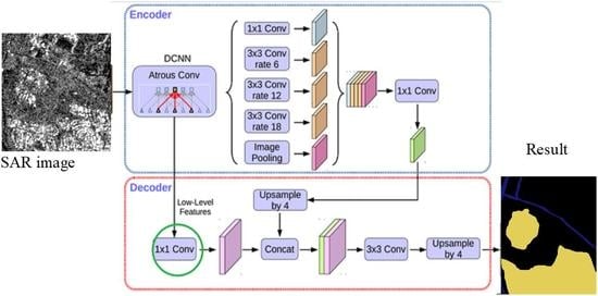
2.1. The Structure of Deeplabv3+ Network

The total structure of the Deeplabv3+ network is shown in Figure 1. Deeplabv3+ extends Deeplabv3 by adding a simple yet effective decoder module to refine the segmentation results, especially along the object boundaries. It includes two parts: the encoder and decoder. The encoder is mainly used for extracting features and reducing the dimensionality of the feature map. The decoder is mainly used to restore the edge information and resolution of the feature map to obtain the final semantic segmentation results. To increase the receptive field and maintain the resolution of the feature map, the convolution operation of the last few convolutional layers of the encoder is replaced with hole convolution. The atrous spatial pyramid pooling (ASPP) module introduced in Deeplabv3+ uses dilation convolution at various rates to obtain multi-scale semantic contextual information. By using these novel structures, Deeplabv3+ produces accurate semantic segmentation results among different datasets.

2.2. Potential Energy Loss Function Based on the Gibbs Distribution

Semantic image segmentation is considered a pixel-wise classification problem in practice, and the most commonly used pixel-wise loss for semantic segmentation is the SoftMax cross-entropy loss in terms of predicted label $y$ and ground truth g, which is:

$$L_{ce}(y,g)=-\frac{1}{M}{\displaystyle \sum _{m=1}^M{\displaystyle \sum _{n=1}^N{y}_{m,n}\log (p_{m,n})}}$$

(1)

Here, $M$ denotes the number of pixels and $N$ denotes the number of object classes. It can be seen from Equation (1) that the pixel-wise loss function calculates the prediction error of a single category independently and ignores the interaction between different feature categories. To exploit the relationship among them, the region mutual information loss function (RMI loss) was proposed [18], which applies mutual information to model the dependencies simply and efficiently.

According to information theory knowledge [19], the mutual information between the two random variable sets $G$ and $Y$ is:

$$I(Y;G)={\displaystyle \sum _{y,g}p(y,g)\log \frac{p(y|g)}{p(y)}}={\displaystyle \sum _{y,g}p(y|g)p(g)\log \frac{p(y|g)}{p(y)}}$$

(2)

If $G$ and $Y$ represent the ground truth and predicted results, respectively, for a given network and dataset,$p(g)$ and $p(y)$ are determined. Hence, $I(Y;G)$ is only related to $p(y|g)$, which is the reason that previous papers approximated the lower bound of $I(Y;G)$ by calculating the conditional entropy between $G$ and $Y$. However, it only calculates $I(Y;G)$ in the neighborhood with a radius of 3 around the central object category. There are different sizes among different object categories in the image. Usually, it is necessary to consider the semantic relationship between different categories in multiple neighborhoods of different sizes. Therefore, based on the neighborhood system $\eta$ and Gibbs clique $c$, we propose a potential energy loss function based on the Gibbs distribution to approximate mutual information $I(Y;G)$. The proposed total loss function based on the Gibbs distribution is as follows:

$$L_{all}(y,g)=\alpha L_{ce}(y,g)+(1-\alpha )I(Y;G)$$

(3)

Here, $\alpha$ is the weight coefficient and the neighbor we use is 4-connected. By modeling Gibbs cliques of different neighborhood systems, the semantic contextual information between different feature categories in different neighborhoods is considered.

Consider a random field $X=\{X_1,X_2,\dots ,X_n\}$, which is defined on the observation sequence sample sets $x=\{x_1,x_2,\dots ,x_n\}$. According to graph theory [20], if a random field satisfies the Markov property $P\left(X_i=x_i|X_k=x_k,k\ne i\right)=P\left(X_i=x_i|X_k=x_k,k\in {\eta }_i\right)$ and translation invariance in the same neighborhood system $\eta$, $X$ can be called a Markov random field (MRF) with $\eta$ as the neighborhood system. Given neighborhood system $\eta$ and Gibbs clique $c$, the Gibbs distribution of the MRF can be described as:

$$P\left(X=x\right)=\frac{1}{Z}\exp \left(-E\left(x\right)\right)$$

(4)

$$E\left(x\right)={\displaystyle \sum _{c\in \xi }{H}_c}\left(X,\theta \right)$$

(5)

$$Z={\displaystyle \sum _x\exp \left(-E(x)\right)}$$

(6)

where $E$ is the sum of the potential energies of different cliques in a single neighborhood system $\eta$; $Z$ is the normalization coefficient; $\theta$ is the model parameter related to the Gibbs clique; $\xi$ is the set of the clique $\eta$; and $H_c$ is the potential energy of clique $c$, which quantitatively describes the relationship between different samples of the random field, as shown in Equation (7):

$$H_c\left(x_o,x_r,\lambda \right)=1-\frac{2}{1+{\left(\left|x_o-x_r\right|/\lambda \right)}^2}$$

(7)

where $x_o$ represents the central sample of $c$, $x_r$ is the sample in the $\eta$ of $x_o$, and $\lambda$ is the parameter related to the observed sequence. For a given observed sequence, $\lambda$ is determined, so it is ignored in the subsequent equations. The multi-size neighborhood system is used to model the observed sequence $x=\{x_1,x_2,\dots ,x_n\}$. The total Gibbs energy of all neighborhood systems is:

$$E(X)={\displaystyle \sum _{r\in \eta }{\theta }_r{\displaystyle \sum _{c\in \xi }{H}_c\left(x_o,x_r\right)}}$$

(8)

where ${\theta }_r$ is the parameter of the corresponding neighborhood system $\eta$, which is a set of weights of different Gibbs cliques in $\eta$. In terms of the potential energy function and Gibbs distribution, the total Gibbs-MRF model is expressed as:

$$P\left(x_o|x_{o+r},r\in \eta \right)=\frac{1}{Z}\exp \left(-{\displaystyle \sum _{r\in \eta }{\theta }_r{\displaystyle \sum _{c\in \xi }{H}_c\left(x_o,x_r\right)}}\right)$$

(9)

Here, random fields $Y$ and $G$ correspond to the sets of random variables $\{y_1,y_2,\dots ,y_k\}$ and $\{g_1,g_2,\dots ,g_k\}$, which represent the predicted results and ground truth corresponding to the observed sequence, respectively. As such, the Gibbs distribution between $Y$ and $G$ can be determined as:

$$P\left(y_o|g_{o+r},r\in \eta \right)=\frac{1}{Z}\exp \left(-E(Y,G|X)\right)$$

(10)

where $\left(E(Y,G|X)\right)$ represents the Gibbs energy between $Y$ and $G$ as given for $X$. For the convenience of understanding, the observed sequence $X$ is ignored in the subsequent expressions as:

$$\begin{array}{cc}E(Y,G)\hfill & ={\displaystyle \sum _{r\in \eta }{\theta }_r{\displaystyle \sum _{c\in \xi }{H}_c\left(y_o,g_{o+r}\right)}}\hfill \\ & ={\displaystyle \sum _{r\in \eta }{\theta }_0{H}_1(y_{\mathrm{o}},g_{\mathrm{o}})}+{\displaystyle \sum _{r\in \eta }{\theta }_r{\displaystyle \sum _{c\in \xi ,c\ne 1}{H}_c\left(y_o,g_r\right)}}\hfill \\ & ={\displaystyle \sum _{r\in \eta }{\theta }_0\{1-\frac{2}{1+{(y_o-g_o)}^2}\}}+{\displaystyle \sum _{r\in \eta }{\theta }_r}{\displaystyle \sum _{c\in \xi ,c\ne 1}\{1-\frac{2}{1+{(y_o-g_r)}^2}\}}\hfill \end{array}$$

(11)

where ${\displaystyle \sum _{r\in \eta }{\theta }_0{H}_1(y_{\mathrm{o}},g_{\mathrm{o}})}$ is the sum of the potential energy of single-element cliques in all neighborhood systems, which reflects the dependencies among single elements between $Y$ and $G$ in different neighborhood systems; ${\displaystyle \sum _{r\in \eta }{\theta }_r{\displaystyle \sum _{c\in \xi ,c\ne 1}{H}_c\left(y_o,g_r\right)}}$ denotes the sum of the potential energy of multi-element cliques between $Y$ and $G$ in all neighborhood systems. The potential energy essentially represents the dependency among different elements of cliques in various neighborhood systems between $Y$ and $G$.

The log transformation of Equation (10) can be expressed as:

$$\log (P\left(y_o|g_{o+r},r\in \eta \right))=\log (\frac{1}{Z}\exp \left(-E(Y,G)\right))=-\log Z-E(Y,G)$$

(12)

Because $Z$ is the normalization coefficient, the Gibbs energy $E(Y,G)$ only depends on $P\left(y_o|g_{o+r},r\in \eta \right)$. The potential energy function based on multi-size neighborhood systems is proposed to approximate the mutual information as:

$$I^{b,n}(Y;G)=-{\displaystyle \sum _{r\in \eta }{\theta }_r{\displaystyle \sum _{c\in \xi }{H}_c\left(y_o,g_r\right)}}$$

(13)

The proposed total potential energy loss function based on the Gibbs distribution can be expressed as:

$$\begin{array}{cc}{L}_{all}(y,g)\hfill & =\alpha L_{ce}(y,g)+(1-\alpha )(-I(Y;G))\hfill \\ & =\alpha L_{ce}(y,g)+(1-\alpha )1/B{\displaystyle \sum _{b=1}^B{\displaystyle \sum _{n=1}^N(-I^{b,n}(Y;G))}}\hfill \\ & =\alpha L_{ce}(y,g)+(1-\alpha )1/B{\displaystyle \sum _{b=1}^B{\displaystyle \sum _{n=1}^N{\displaystyle \sum _{r\in \eta }{\theta }_r{\displaystyle \sum _{c\in \xi }{H}_c\left(y_o,g_r\right)}}}}\hfill \end{array}$$

(14)

Here, $B$ denotes the number of images in a mini-batch.

2.3. Improved Channel Spatial Attention Module (CBAM)

The attention module in deep learning is proposed based on human visual attention. It pays more attention to the important features while ignoring some related but low-contributing features. The original CBAM directly inputs the result of the channel attention module to the spatial attention module and loses the spatial contextual information among different categories of the feature map. Therefore, we add the original feature map and the result of the channel attention, then input that to the spatial attention module, which supplements the spatial feature information lost by the channel attention module to some extent. The overall structure is shown in Figure 2. Our modification is shown with a red line.

The channel attention module first performs global average pooling and global maximum pooling on the input feature map $F$, then the output passes through two fully connected layers, separately. The sigmoid function is used to normalize the output in the end. The entire process can be expressed as follows: Our improvement is shown in Equation (18), which adds the original feature map to the channel attention result.

$$F_{avg}^c=\frac{1}{W\ast H}{\displaystyle \sum _{i=1}^W{\displaystyle \sum _{j=1}^{H}F(i,j)}}$$

(15)

$$F_{\max }^c=\max (F(i,j):i\in W,j\in H)$$

(16)

$$W^c=Sigmoid(FC2(ReLU(FC1(F_{avg}^c+F_{\max }^c))))$$

(17)

$$F^{\prime }=W_{out}^c=F\ast W^c+F$$

(18)

where $W$ and $H$ represent the width and height of $F$, respectively; $FC1$ and $FC2$ both represent a fully connected layer; $Sigmoid$ and $ReLU$ both represent the nonlinear activation function. The final output of channel attention is $F^{\prime }$.

The spatial attention module mainly focuses on the spatial area, which places the most impact on the final result, which calculates the average value and maximum value of $F^{\prime }$ among all channels first, then stitches them in the channel dimension. After a convolution operation, the output is normalized through a sigmoid function as:

$$F^{″}=W_{out}^s=F^{\prime }\ast Conv(cat(max(F^{\prime }),mean(F^{\prime }),\dim =1))$$

(19)

where dim = 1 represents the channel dimension and $F^{″}$ represents the final output of our improved CBAM.

3. Results and Analysis

In this section, we first introduce the dataset and metrics used to train and test the model. Afterward, the experiments conducted to test the efficiency of the proposed method are described. The experiment results demonstrated that the proposed method increases both the GA and mIoU with a faster running time and obtains a state-of-the-art result.

3.1. Dataset

The SAR images were taken by the Sentinel-1 satellite with a resolution of 10 m, and the size of the SAR images was 256 × 256. We manually labeled the SAR images with the LabelMe labeling software into five pixels categories: background (cls0, black), river (cls1, red), plain (cls2, green), building (cls3, yellow), and road (cls4, blue). We used some enhancement operations such as rotation and image transformation to enhance our dataset. The total number of the whole dataset is 2800 image-label pairs. We randomly selected 2000 pairs as the training set and 800 pairs as the validation set. The original images, which were 8-bit grayscale imagery, and their corresponding ground truths, are shown in Figure 3.

3.2. Implement Details

We conducted the experiments based on the platform PyTorch, and all experiments were conducted on a workstation with RTX 2080 Ti Graphic Processing Unit (GPU) cards under Compute Unified Device Architecture (CUDA) 10.0. The Adam optimizer [21] was used to train the network for a total of 800 epochs with a batch size of 16 and an initial learning rate of 0.003. The initial learning rate was multiplied by ${(1-\frac{iter}{\max \_iter})}^{power}$ at a different training iteration, where the power was 0.9 [14]. The potential energy loss function based on the Gibbs distribution proposed in Section 2.2 was used to train the model. To obtain a quantitative evaluation result, we adopted GA, intersection over union (IoU), and mean Intersection over Union (mIoU) as metrics, which are:

$$GA={\displaystyle \sum _{i=1}^k{n}_{ii}}/{\displaystyle \sum _{i=1}^k{t}_i}$$

(20)

$$Io{U}_{cls}=\frac{n_{ii}}{t_i-n_{ii}+{\displaystyle \sum _j^k{n}_{ji}}}$$

(21)

$$mIo{U}_{cls}=\frac{1}{k}{\displaystyle \sum _{i=1}^k\frac{n_{ii}}{t_i-n_{ii}+{\displaystyle \sum _{j=1}^k{n}_{ji}}}}$$

(22)

where $t_i$ is the total number of pixels of class $i$ and the subscript $cls$ means the accuracy within the specific class. $k$ is the number of classes and $n_{ij}$ is the number of pixels that belong to class $i$ and were classified as class $j$. The convergence of loss function and change of $mIo{U}_{cls}$ during the training and validation is shown in Figure 4.

Figure 4 shows that the value of the proposed loss function decreases with the training of the network, indicating that the entire network continues to converge during the training process. In the later stage of training, the value of the loss function changed little, indicating that the network was stable. According to Equation (14), the value of the loss function mainly depends on the proposed potential loss function, and the detailed calculation is given in Equation (11), which shows that the value should be negative and the smaller the network prediction error, the larger the absolute value of the loss function, which matches the curve well. $mIo{U}_{cls}$ increased with the training of the network, and finally reached a stable value.

Table 1. The metrics results of our method.

$G{A}_{train}$	$G{A}_{val}$	$Io{U}_{cls0}$	$Io{U}_{cls1}$	$Io{U}_{cls2}$	$Io{U}_{cls3}$	$Io{U}_{cls4}$	$mIo{U}_{cls}$
90.90%	90.27%	97.20%	96.63%	95.92%	88.80%	46.84%	85.08%

shows the final metrics values of our proposed method, showing that the proposed method achieves ideal results. $G{A}_{train}$ and $G{A}_{val}$ represent the Global Accuracy of the train set and val set.

3.3. Ablation Study

This section empirically shows the effectiveness of our design choice. Firstly, we searched for the effective backbone Mobilenetv2 used in the Deeplabv3+ network, then compared the results of different networks with the proposed potential energy loss function and the cross-entropy loss function, separately. The influence of different weight coefficients $\alpha$ in the proposed loss function was compared, and the proposed loss function was compared with the RMI loss function based on the same Deeplabv3+–Mobilenetv2 network as well. Finally, we searched for the effectiveness of the improved CBAM on SAR imagery semantic segmentation.

3.3.1. Designing the Network for SAR Imagery Semantic Segmentation

Considering the efficiency of the Deeplabv3+ network used for semantic image segmentation, we applied it to semantically segment SAR imagery in this study. Because the SAR dataset labeled by us was small, Deeplabv3+ with an efficient Mobilenetv2 backbone was designed as the base network. To verify the effectiveness of the design choice, this section compares the Deeplabv3+–Mobilenetv2 with Deeplabv3+–ResNet, Deeplabv3+–drn [22], FCN, and PSPNet, which are trained based on the cross-entropy loss function. The metrics results of these networks are shown in Table 2.

Table 2. The metrics results and test time of several networks based on the cross-entropy loss function.

Network	$\mathit{G}{\mathit{A}}_{\mathit{V}\mathit{a}\mathit{l}}$	$\mathit{I}\mathit{o}{\mathit{U}}_{\mathit{c}\mathit{l}\mathit{s}0}$	$\mathit{I}\mathit{o}{\mathit{U}}_{\mathit{c}\mathit{l}\mathit{s}1}$	$\mathit{I}\mathit{o}{\mathit{U}}_{\mathit{c}\mathit{l}\mathit{s}2}$	$\mathit{I}\mathit{o}{\mathit{U}}_{\mathit{c}\mathit{l}\mathit{s}3}$	$\mathit{I}\mathit{o}{\mathit{U}}_{\mathit{c}\mathit{l}\mathit{s}4}$	$\mathit{m}\mathit{I}\mathit{o}{\mathit{U}}_{\mathit{c}\mathit{l}\mathit{s}}$	Time
PSPNet [11]	60.93%	90.22%	83.14%	47.02%	53.76%	40.75%	54.98%	3.13s
FCN [9]	68.99%	90.10%	87.39%	59.83%	63.33%	17.10%	63.55%	3.03s
Deeplabv3+ –Resnet [15]	72.83%	92.14%	87.34%	85.98%	73.20%	0	67.73%	4.52s
Deeplabv3+ –drn [22]	70.77%	91.95%	89.04%	84.51%	70.99%	0	66.94%	3.65s
Deeplabv3+ –Mobilenetv2 [16]	73.37%	92.51%	87.38%	88.36%	73.18%	0	68.28%	2.94s

Table 2. The metrics results and test time of several networks based on the cross-entropy loss function.

Network	$\mathit{G}{\mathit{A}}_{\mathit{V}\mathit{a}\mathit{l}}$	$\mathit{I}\mathit{o}{\mathit{U}}_{\mathit{c}\mathit{l}\mathit{s}0}$	$\mathit{I}\mathit{o}{\mathit{U}}_{\mathit{c}\mathit{l}\mathit{s}1}$	$\mathit{I}\mathit{o}{\mathit{U}}_{\mathit{c}\mathit{l}\mathit{s}2}$	$\mathit{I}\mathit{o}{\mathit{U}}_{\mathit{c}\mathit{l}\mathit{s}3}$	$\mathit{I}\mathit{o}{\mathit{U}}_{\mathit{c}\mathit{l}\mathit{s}4}$	$\mathit{m}\mathit{I}\mathit{o}{\mathit{U}}_{\mathit{c}\mathit{l}\mathit{s}}$	Time
PSPNet [11]	60.93%	90.22%	83.14%	47.02%	53.76%	40.75%	54.98%	3.13s
FCN [9]	68.99%	90.10%	87.39%	59.83%	63.33%	17.10%	63.55%	3.03s
Deeplabv3+ –Resnet [15]	72.83%	92.14%	87.34%	85.98%	73.20%	0	67.73%	4.52s
Deeplabv3+ –drn [22]	70.77%	91.95%	89.04%	84.51%	70.99%	0	66.94%	3.65s
Deeplabv3+ –Mobilenetv2 [16]	73.37%	92.51%	87.38%	88.36%	73.18%	0	68.28%	2.94s

Table 2 shows that regardless of the backbone network is used, the road in the SAR images cannot be recognized, but the recognition accuracy for other object categories such as buildings and plains is high. Although FCN and PSPNet networks can recognize roads, the recognition accuracy of the other object categories is lower than that of the Deeplabv3+ network, and the $mIo{U}_{cls}$ is much smaller than that of the Deeplabv3+ network, which verifies the effectiveness of choosing Deeplabv3+ for SAR imagery semantic segmentation. It only takes 2.94 s for Deeplabv3+–Mobilenetv2 to obtain the $mIo{U}_{cls}$ of 68.28%, which is 1.34% higher than that of Deeplabv3+–drn and 0.55% higher than that of Deeplabv3+–Resnet in less time, verifying the design choice of Mobilenetv2 as the backbone. Figure 5 visualizes the prediction results of the five networks. The fifth row of Figure 5 shows that although Deeplabv3+–Mobilenetv2 cannot recognize roads, the recognition result of other object categories is the closest to the ground truth.

3.3.2. The Potential Energy Loss Function Based on the Gibbs Distribution

Table 2 and Figure 5 shows that the five networks cannot recognize roads in SAR imagery, potentially due to the complex structure of SAR imagery and the existence of speckle noise. However, the main reason is that the pixel-wise cross-entropy loss function only considers single categories and ignores the semantic relationship among different categories. The network was trained with the potential energy loss function based on the Gibbs distribution proposed in Section 2.2, where the parameter ${\theta }_r$ is a set of weights of different Gibbs cliques in the neighborhood system, which is always near 1 based on the calculation of the proposed loss function and the model settings. The value of the parameter ${\theta }_r$ was set to 1 in all our experiments and the weighting coefficient $\alpha$ was set to 0.5. The metrics results are shown in

Table 3. The results of the three networks based on the proposed potential energy loss function.

Network	$\mathit{G}{\mathit{A}}_{\mathit{V}\mathit{a}\mathit{l}}$	$\mathit{I}\mathit{o}{\mathit{U}}_{\mathit{c}\mathit{l}\mathit{s}0}$	$\mathit{I}\mathit{o}{\mathit{U}}_{\mathit{c}\mathit{l}\mathit{s}1}$	$\mathit{I}\mathit{o}{\mathit{U}}_{\mathit{c}\mathit{l}\mathit{s}2}$	$\mathit{I}\mathit{o}{\mathit{U}}_{\mathit{c}\mathit{l}\mathit{s}3}$	$\mathit{I}\mathit{o}{\mathit{U}}_{\mathit{c}\mathit{l}\mathit{s}4}$	$\mathit{m}\mathit{I}\mathit{o}{\mathit{U}}_{\mathit{c}\mathit{l}\mathit{s}}$	Time
Deeplabv3+–Resnet	86.46%	96.45%	95.35%	95.02%	85.52%	36.84%	81.84%	4.45 s
Deeplabv3+–drn	90.80%	97.19%	96.69%	95.46%	88.99%	50.32%	85.73%	3.82 s
Deeplabv3+–Mobilenetv2	90.27%	97.18%	96.85%	95.64%	88.60%	46.69%	84.99%	2.83 s

.

Comparing Table 2 and Table 3, the proposed loss function qualitatively improves the recognition accuracy of networks, especially for roads. The recognition of roads based on Deeplabv3+–Mobilenetv2 increases from 0% to 46.69%, the $mIo{U}_{cls}$ of Deeplabv3+–Mobilenetv2 increases from 68.28% to 84.99%, and the time is reduced by 0.11 s. Although the performance of the Deeplabv3+–drn is better than that of Deeplabv3+–Mobilenetv2, it is slower. To achieve better performance with less time consumed, Deeplabv3+–Mobilenetv2, based on the proposed potential energy loss function, was introduced in this study to semantically segment SAR imagery. Figure 6 shows the results of the three networks based on the proposed loss function. Comparing Figure 5 and Figure 6, the results of three networks based on our proposed loss function are both clearer than those based on cross-entropy loss function regardless of object category, and Deeplabv3+–Mobilenetv2 achieved the clearest results of the three networks.

3.3.3. Influence of Weighting Coefficient $\alpha$ Compared with RMI Loss Function

In the previous experiments, the weighting coefficient $\alpha$ was set to 0.5. To test the influence of different $\alpha$ values on the prediction result of Deeplabv3+–Mobilenetv2, the value of $\alpha$ was set to 0.25, 0.5, and 0.75, separately, for comparison. In addition, we compared the RMI loss function with the same parameters as previous papers and the proposed potential energy loss function used on the same Deeplabv3+–Mobilenetv2. The metrics results are shown in

Table 4. The metrics results of Deeplabv3+–Mobilenetv2 under different conditions.

Method	$\mathit{G}{\mathit{A}}_{\mathit{V}\mathit{a}\mathit{l}}$	$\mathit{I}\mathit{o}{\mathit{U}}_{\mathit{c}\mathit{l}\mathit{s}0}$	$\mathit{I}\mathit{o}{\mathit{U}}_{\mathit{c}\mathit{l}\mathit{s}1}$	$\mathit{I}\mathit{o}{\mathit{U}}_{\mathit{c}\mathit{l}\mathit{s}2}$	$\mathit{I}\mathit{o}{\mathit{U}}_{\mathit{c}\mathit{l}\mathit{s}3}$	$\mathit{I}\mathit{o}{\mathit{U}}_{\mathit{c}\mathit{l}\mathit{s}4}$	$\mathit{m}\mathit{I}\mathit{o}{\mathit{U}}_{\mathit{c}\mathit{l}\mathit{s}}$	Time
$\alpha =0.25$	89.62%	97.15%	96.69%	95.69%	88.57%	45.15%	84.65%	2.84 s
$\alpha =0.5$	90.27%	97.18%	96.85%	95.64%	88.60%	46.69%	84.99%	2.83 s
$\alpha =0.75$	89.15%	97.17%	96.92%	95.79%	88.37%	42.66%	84.19%	2.86 s
RMI loss	88.05%	96.63%	96.30%	95.09%	86.26%	37.08%	82.27%	2.93 s

.

Table 4 shows that the results of Deeplabv3+–Mobilenetv2 based on the potential energy loss function are roughly the same despite different $\alpha$ coefficients. $mIo{U}_{cls}$ is the highest and the time consumed is the least with $\alpha =0.5$, so we set $\alpha$ to 0.5. The $Io{U}_{cls4}$ and $mIo{U}_{cls}$ of Deeplabv3+–Mobilenetv2 based on our proposed loss function were 9.61% and 2.72% higher than that based on RMI loss function, respectively, and the method proposed in this paper consumes less time. The results shown here verify the high efficiency of the proposed method furthermore.

3.3.4. The Influence of Improved CBAM

In this section, the results of Deeplabv3+–Mobilenetv2 with the improved CBAM and the original CBAM are compared. The proposed potential energy loss function based on the Gibbs distribution was used to train the network, and the metrics results are shown in

Table 5. The metrics results of Deeplabv3+–Mobilenetv2 with CBAM and without CBAM.

Method	$\mathit{G}{\mathit{A}}_{\mathit{V}\mathit{a}\mathit{l}}$	$\mathit{I}\mathit{o}{\mathit{U}}_{\mathit{c}\mathit{l}\mathit{s}0}$	$\mathit{I}\mathit{o}{\mathit{U}}_{\mathit{c}\mathit{l}\mathit{s}1}$	$\mathit{I}\mathit{o}{\mathit{U}}_{\mathit{c}\mathit{l}\mathit{s}2}$	$\mathit{I}\mathit{o}{\mathit{U}}_{\mathit{c}\mathit{l}\mathit{s}3}$	$\mathit{I}\mathit{o}{\mathit{U}}_{\mathit{c}\mathit{l}\mathit{s}4}$	$\mathit{m}\mathit{I}\mathit{o}{\mathit{U}}_{\mathit{c}\mathit{l}\mathit{s}}$	Time
No-CBAM	90.27%	97.18%	96.85%	95.64%	88.60%	46.69%	84.99%	2.83 s
Origin CBAM	89.24%	97.09%	96.90%	95.38%	88.06%	44.64%	84.41%	2.86 s
Improved CBAM	90.57%	97.20%	96.63%	95.92%	88.80%	46.84%	85.08%	2.94 s

.

The results in Table 5 show that Deeplabv3+–Mobilenetv2 with the improved CBAM achieves better results than the original CBAM with a 0.67% higher $mIo{U}_{cls}$, while the testing time was 0.11 s longer, mainly because we added the feature map and the result of channel attention module directly, increasing the feature redundancy. In addition, our proposed potential energy loss function achieves the attention effect to some extent, and the result of original Deeplabv3+–Mobilenetv2 is suitable to some extent, so the improvement of adding the proposed CBAM to Deeplabv3+–Mobilenetv2 is not obvious.

4. Discussion and Conclusions

The Deeplabv3+ network with an efficient Mobilenetv2 backbone was introduced in this paper to semantically segment SAR imagery. This method uses the proposed potential energy loss function based on the Gibbs distribution to model the dependencies among different categories efficiently. To obtain higher recognition accuracy of small object categories, an improved CBAM was introduced to Deeplabv3+–Mobilenetv2 and achieved better results to some extent. The experiment results showed that the proposed method for SAR imagery semantic segmentation is effective, especially the proposed potential energy loss function, which can be effectively used with any existing network. Although the improved CBAM module has a positive effect on the accuracy of the model, the improvement is not obvious, and the time consumed increases with the added CBAM module. In future work, we will focus on the more efficient ways to improve the CBAM attention module and some efficient methods to enhance the SAR imagery.

References

1. Yang, W.; Zhang, X.; Chen, L.; Hong, S. Semantic Segmentation of Polarimetric SAR Imagery Using Conditional Random Fields. In Proceedings of the 2010 IEEE Geoscience & Remote Sensing Symposium, Honolulu, HI, USA, 25–30 July 2010. [Google Scholar]
2. Zhou, Y.; Wang, H.; Xu, F.; Jin, Y.Q. Polarimetric SAR Image Classification Using Deep Convolutional Neural Networks. IEEE Geosci. Remote Sens. Lett. 2017, 13, 1935–1939. [Google Scholar] [CrossRef]
3. Lee, J.S.; Jurkevich, I. Segmentation of SAR images. IEEE Trans. Geosci. Remote Sens. 1989, 27, 674–680. [Google Scholar] [CrossRef]
4. Ji, J.; Wang, K.L. A robust nonlocal fuzzy clustering algorithm with between-cluster separation measure for SAR image segmentation. IEEE J. Sel. Top. Appl. Earth Observ. Remote Sens. 2014, 7, 4929–4936. [Google Scholar] [CrossRef]
5. Yu, H.; Zhang, X.; Wang, S.; Hou, B. Context-based hierarchical unequal merging for SAR image segmentation. IEEE Trans. Geosci. Remote Sens. 2013, 51, 995–1009. [Google Scholar] [CrossRef]
6. Krizhevsky, A.; Sutskever, I.; Hinton, G. ImageNet Classification with Deep Convolutional Neural Networks. In Proceedings of the NIPS’12: 25th International Conference on Neural Information Processing Systems, Lake Tahoe, 3–6 December 2012; Curran Associates, Inc.: Red Hook, NY, USA, 2012; Volume 60. [Google Scholar]
7. Szegedy, C.; Liu, W.; Jia, Y.; Sermanet, P.; Reed, S.; Anguelov, D.; Erhan, D.; Vanhoucke, V.; Rabinovich, A. Going Deeper with Convolutions. In Proceedings of the IEEE Conference on Computer Vision and Pattern Recognition, Boston, MA, USA, 7–12 June 2015. [Google Scholar]
8. Farabet, C.; Couprie, C.; Najman, L.; LeCun, Y. Learning Hierarchical Features for Scene Labeling. IEEE Trans. Pattern Anal. Mach. Intell. 2013, 35, 1915–1929. [Google Scholar] [CrossRef] [Green Version]
9. Shelhamer, E.; Long, J.; Darrell, T. Convolutional Networks for Semantic Segmentation. IEEE Trans. Pattern Anal. Mach. Intell. 2015, 39, 640–651. [Google Scholar] [CrossRef]
10. Liang, X.; Liu, S.; Shen, X.; Yang, J.; Liu, L.; Dong, J.; Lin, L.; Yan, S. Deep Human Parsing with Active Template Regression. IEEE Trans. Pattern Anal. Mach. Intell. 2015, 37, 2402–2414. [Google Scholar] [CrossRef] [Green Version]
11. Zhao, H.; Shi, J.; Qi, X.; Wang, X.; Jia, J. Pyramid Scene Parsing Network. In Proceedings of the 2017 IEEE Conference on Computer Vision and Pattern Recognition, Honolulu, HI, USA, 21–26 July 2017. [Google Scholar]
12. Duan, Y.; Tao, X.; Han, C.; Qin, X.; Lu, J. Multi-scale Convolutional Neural Network for SAR Image Semantic Segmentation. In Proceedings of the IEEE International Conference on Computer Vision, Abu Dhabi, UAE, 9–13 December 2018; Volume 2, pp. 941–947. [Google Scholar]
13. Zhang, Z.; Guo, W.; Yu, W.; Yu, W. Multi-task fully convolutional networks for building segmentation on SAR image. In Proceedings of the IET International Radar Conference (IRC 2018), Nanjing City, China, 17–19 October 2018; Volume 2019, pp. 7074–7077. [Google Scholar]
14. Chen, L.C.; Zhu, Y.; Papandreou, G.; Schroff, F.; Adam, H. Encoder-Decoder with Atrous Separable Convolution for Semantic Image Segmentation. In Proceedings of the 15th European Conference on Computer Vision (ECCV), Munich, Germany, 8–14 September 2018. [Google Scholar]
15. He, K.; Zhang, X.; Ren, S.; Sun, J. Deep Residual Learning for Image Recognition. In Proceedings of the IEEE Conference on Computer Vision and Pattern Recognition, Las Vegas, NV, USA, 27–30 June 2016. [Google Scholar]
16. Sandler, M.; Howard, A.; Zhu, M.; Zhmoginov, A.; Chen, L.C. MobileNetV2: Inverted Residuals and Linear Bottlenecks. In Proceedings of the IEEE Conference on Computer Vision and Pattern Recognition, Salt Lake City, UT, USA, 18–23 June 2018. [Google Scholar]
17. Woo, S.; Park, J.; Lee, J.Y.; So Kweon, I. In So Kweon. CBAM: Convolutional Block Attention Module. In Proceedings of the European Conference on Computer Vision (ECCV), Munich, Germany, 8–14 September 2018; Springer Healthcare: New York, NY, USA, 2018. [Google Scholar]
18. Zhao, S.; Wang, Y.; Yang, Z.; Cai, D. Region Mutual Information Loss for Semantic Segmentation. In Advances in Neural Information Processing Systems; MIT Press: Cambridge, UK, 2019. [Google Scholar]
19. Cover, M.T.; Thomas, J.A. Elements of Information Theory, 2nd ed.; John Wiley & Sons: Hoboken, NJ, USA, 2006. [Google Scholar]
20. Koller, D.; Friedman, N. Probabilistic Graphical Models: Principles and Techniques; MIT Press: Cambridge, MA, USA, 2009. [Google Scholar]
21. Kingma, D.P.; Ba, J. Adam: A Method for Stochastic Optimization; ICLR: New Orleans, LA, USA, 2015. [Google Scholar]
22. Yu, F.; Koltun, V.; Funkhouser, T. Dilated Residual Networks. In Proceedings of the IEEE Conference on Computer Vision and Pattern Recognition, Honolulu, HI, USA, 21–26 July 2017. [Google Scholar]
Figure 1. The structure of the Deeplabv3+ network.
Remotesensing 13 00454 g001
Figure 2. The channel and spatial attention module.
Remotesensing 13 00454 g002
Figure 3. The SAR imagery and its corresponding ground truth: (a) SAR imagery; (b) ground truth.
Remotesensing 13 00454 g003
Figure 4. (a) The convergence of the proposed loss function; (b) the change in m I o U c l s .
Remotesensing 13 00454 g004
Figure 5. The results of different networks: (a) SAR images; (b) ground truth; (c) Deeplabv3+–drn output; (d) Deeplabv3+–ResNet output; (e) Deeplabv3+–Mobilenetv2 output; (f) PSPNet output; (g) FCN output.
Remotesensing 13 00454 g005aRemotesensing 13 00454 g005b
Figure 6. The results of the three different networks: (a) SAR imagery; (b) ground truth; (c) Deeplabv3–drn output; (d) Deeplabv3–ResNet output; (e) Deeplabv3–Mobilenetv2 output.
Remotesensing 13 00454 g006