Article

Spatial Allocation Method from Coarse Evapotranspiration Data to Agricultural Fields by Quantifying Variations in Crop Cover and Soil Moisture

1
State Key Laboratory of Remote Sensing Science, Aerospace Information Research Institute, Chinese Academy of Sciences, Beijing 100101, China
2
College of Resources and Environment, University of Chinese Academy of Sciences, Beijing 100101, China
*
Author to whom correspondence should be addressed.
Remote Sens. 2021, 13(3), 343; https://doi.org/10.3390/rs13030343
Submission received: 8 December 2020 / Revised: 18 January 2021 / Accepted: 18 January 2021 / Published: 20 January 2021
(This article belongs to the Special Issue Remote Sensing in Hydrology and Water Resources Management)

Abstract

:
Cropland evapotranspiration (ET) is the major source of water consumption in agricultural systems. The precise management of agricultural ET helps optimize water resource usage in arid and semiarid regions and requires field-scale ET data support. Due to the combined limitations of satellite sensors and ET mechanisms, the current high-resolution ET models need further refinement to meet the demands of field-scale ET management. In this research, we proposed a new field-scale ET estimation method by developing an allocation factor to quantify field-level ET variations and allocate coarse ET to the field scale. By regarding the agricultural field as the object of the ET parcel, the allocation factor is calculated with combined high-resolution remote sensing indexes indicating the field-level ET variations under different crop growth and land-surface water conditions. The allocation ET results are validated at two ground observation stations and show improved accuracy compared with that of the original coarse data. This allocated ET model provides reasonable spatial results of field-level ET and is adequate for precise agricultural ET management. This allocation method provides new insight into calculating field-level ET from coarse ET datasets and meets the demands of wide application for controlling regional water consumption, supporting the ET management theory in addressing the impacts of water scarcity on social and economic developments.

Graphical Abstract

1. Introduction

Land evapotranspiration (ET) is a major component of terrestrial water cycling and groundwater consumption [1]. For basin-scale water balance, the major component of basin water output is ET, followed by surface runoff and infiltration. It is estimated that nearly 70% of the total land precipitation and inflow is returned to the air by terrestrial ET. From an agricultural water management perspective, ET is an important indicator of cropland water consumption and water resource investment [2]. In arid and semiarid regions, social and economic development is limited by the amount of available fresh water [3], and water quotas for agricultural irrigation systems need judicious management, where the balance between irrigation water supply and necessary crop water demand is optimally controlled to maintain normal production [4]. The accurate and timely acquisition of crop ET is critical for reflecting the status of cropland water and determining irrigation strategies [5]. Moreover, views on water management have shifted from the conventional focus on increasing water income and cutting expenditures to the current focus on controlling water consumption. The applications of ET-based water management and a water consumption-oriented water rights allocation system have been demonstrated to be effective in the Turpan Basin, China, which has raised the demand for high-accuracy and low-cost farm-level ET monitoring methods [6,7].
With its broad spatial coverage and high temporal resolution, remote sensing (RS) technology provides a feasible approach to frequently monitor regional ET at low costs and with high efficiency [8]. Accurate surface vegetation cover, albedo, and temperature data provide a solid foundation for the simulation of ET-related physical and physiological processes [9]. Many RS-based ET models have been developed and applied at global and regional scales depending on multiple theories, including the ETWatch model based on the parametrized surface energy balance theory [10], the MOD16 series product based on the global MODIS satellite data and meteorological data [11], the GLEAM product based on the water balance theory [12], and the PML ET product focused on the plant water carbon stomata mechanism [13]. These RS-based ET products provide regional and global ET results at daily or eight-day intervals with moderate spatial resolutions, usually at 500-m to one-km scales. Such ET data have been adopted for studying regional ecological impacts on water resources [14,15,16], modeling land-surface processes [17], analyzing water cycling, and evaluating regional available water resources [16]. However, the spatial scales of these moderate-resolution ET products are too coarse for agricultural water management, especially within small irrigation districts that usually occupy tens to hundreds of square meters, and detailed spatial information is omitted from km-level ET data. Ground-level field ET measurement methods, such as lysimeters, sap flows, and eddy covariances (ECs), are high in cost and require careful management [18]. The combination of precise agricultural ET management and RS technology has developed a strong demand for ET models that show detailed cropland water consumption at the field scale.
Due to the limitations of satellite sensors, high-resolution spatial data usually have long temporal intervals, such as the Landsat series at 30-m resolution and 16-day intervals and the Sentinel-2 data at 10–60-m resolutions and five-day intervals. For agricultural ET monitoring and water consumption applications, the daily scale is ideal for timely evaluations and adjustments of agricultural activities [8]. Considering the impacts of clouds on optical RS data, the temporal gap could be 10 days or even longer. Such long temporal intervals are not satisfactory in many RS-based ET models, and daily ET variations could accumulate and lead to large errors in the monthly and crop ET estimates during growing seasons. The current km-level RS-based ET models are widely applied and highly accurate, and these models help address the limitations of field ET estimation and provide insights into agricultural water applications. Restrained by the inability of high-resolution satellite sensors to meet temporal requirements, the calculation of fine-resolution ET inevitably relies on data downscaling methods that combine high- and low-resolution RS datasets. The downscaling methods mainly focus on the pixel level of satellite images [19].
Most ET downscaling is conducted by downscaling the major parameters in the ET calculation procedure and is combined with other available fine-resolution input data to directly calculate high-resolution ET results. The DisALEXI model is an example of using high-resolution surface temperature to produce a downscaled surface ET [20]. DisALEXI has developed a framework of ET downscaling algorithm, which is to build up a linkage of key parameters between coarse and high-resolution RS data, such as land surface temperature (LST) and normalized difference vegetation index (NDVI) or other vegetation indexes [20,21,22,23]. The downscaling of LST has benefited from multiple research developments on the downscaling of Landsat thermal bands combined with MODIS LST data [24,25,26], such as the thermal sharpening (TSP), land surface temperature disaggregation (DLST), and temperature unmixing (TUM) methods [27,28]. LST downscaling methods are abundantly developed using multiple spatial, temporal, and spectral resolution RS data. However, the scale effects on the LST data and the unstable relationship of intermediate parameters with LST have limited the improvement of the input data accuracy and, thus, limited the LST-based downscaling model [29]. Since crop transpiration processes are accompanied by variability in crop photosynthetic processes [13] and can be monitored with high-resolution optical satellite data, crop transpiration can be estimated with stomatal behavior and biophysical conditions combined with meteorological data. The surface resistance (rs) is an important factor in calculating daily ET and can be downscaled using one-km rs combined with 30-m satellite data and then input into the ET calculations. The downscaling of rs provides fine-resolution information for the ET calculations and is regarded as the basic approach to the spatial monitoring of ET for field-scale management. Studies have shown that the rs-based ET downscaling approach requires the underlying surfaces to be covered with some amount of plants, since its feasibility depends on the biophysical activities of plants’ transpiration through the stomata. For sparsely vegetated regions, the accuracy of the rs-based ET downscaling approach is limited [21]. Those algorithms focus on the relationship of each coarse resolution (m3) pixel and fine resolution (m1) pixels within it; the relationships of adjacent fine resolutions from different coarse pixels are hardly considered, which could bring in some “edges”, as shown in Tan, Wu and Yan’s [21] downscaling results.
Distinguished from pixel-level ET downscaling, the agricultural fields can be regarded as objects that have homogeneous ET properties within each field and heterogeneous properties between the fields. Studies on the ET mechanism and impact analysis of factors on ET have revealed that ET is highly correlated with vegetation cover, soil moisture, air temperature, and vapor pressure deficiency [14,15]. ET can vary among fields due to differences in the soil moisture from irrigation, the transpiration abilities of different crop breeds, fertilization, and growth conditions; thus, it is possible to use the differences in soil water conditions and crop conditions as indicators of the ET differences between fields. At different scales, ET impact factors can vary, and some of these factors can be acquired from high-resolution RS data; this suggests possible approaches in which the field ET within coarse ET pixels could be allocated by means of building relationships between impact factors and ET at the field scale. Combining high-resolution RS data and moderate-resolution actual ET products, field-scale actual ET can be calculated and applied for crop water monitoring. We chose the ETWatch model as the moderate-resolution ET data, as ETWatch is reliable for daily and monthly ET estimations across different climate types and surface characteristics, especially in cropland regions. Its accuracy has been proven by more than 50 research groups for water consumption structure and agricultural irrigation management, including our research region, Haihe Basin and Heihe Basin [7,8,14,16,30]. For ET calculations at high resolution, ETWatch has also been used as input data in several researches, including some downscaling methods [19,21].
To explore the appropriate methods of field ET monitoring and irrigation evaluation, we discuss whether the field ET allocation method combining moderate-resolution ET data and high-resolution satellite data is applicable. The model results are compared with ground ET observations from two typical cropland stations in the North China Plain and Northeast China, both of which are located in arid to semiarid regions. In this research, a total of two years of Sentinel-2 optical data and coarse ET products from the ETWatch model are combined with observations from two ground stations: Guantao from the Haihe Basin, North China Plain and Daman from the Heihe Basin, Northwest China. In Section 2, the data, proposed model, and other research methods are described in detail. Section 3 presents the model results and evaluation. Section 4 discusses the performance of the model and its potential application in field-scale agricultural water management.

2. Materials and Methods
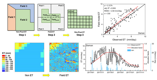
2.1. Method

Figure 1 shows the flowchart of the allocation method from 1 km ET data to agricultural field scale. The crop growth conditions and field moistures are associated with the crop transpiration capacity based on the stomatal behavior and soil water status, and both influence the field ET. In our research, we neglected the possible transport of the horizontal water vapor of adjacent fields; currently, horizonal vapor is analyzed on a large scale, such as the global and continent levels [31]. Most of the current ET RS models have not taken into account that the vapor amount moves horizontally, possibly due to the difficulty in monitoring and estimating horizonal vapors at the regional level. Thus, we assumed that the 1-km ET input data are accurate enough for allocation. One of our research regions, Daman, is located in the Zhangye Oasis, Heihe Basin. The oasis effect of the meteorological parameter differences between an oasis and desert may affect the accuracy of allocation results in heterogeneous regions [32]. To avoid the potential impact of the oasis effect, we limited our research region to a cropland area close to the center of the oasis.
Based on the two classes of virtually unchanged and field-variant parameters that influence the ET, the ET capacity of each field can be evaluated. Thus, we can assume that, between adjacent fields within a coarse ET pixel, some allocation factors derived from the field-variant parameters can be regarded as equivalent to the ET capacity of each field. The relation above can be summarized using the following equation:
ET field 1 : ET field 2 : ET field i = A F f i e l d 1 : A F f i e l d 2 : A F f i e l d i
where ET field i represents the ET of the ith field (i = 1, 2, ··· n) within each coarse ET pixel, and A F f i e l d i represents the allocation factor of the field i (i = 1, 2, ··· n) within each coarse ET pixel. Additionally, the relationship between the ET of field i and the coarse ET pixel can be expressed as follows:
ET field i ET coarse = A F f i e l d i A F c o a r s e
where A F c o a r s e represents the mean allocation factor of the coarse pixel. With Equation (2), each field ET within the coarse ET pixel can be calculated based on the allocation factor, which can also be regarded as the allocation of the coarse pixel-level ET (approximately 1-km level) to the farm-level (10 m level) ET. In the actual practice of field ET allocation, the allocation factor should be calculated from high-resolution RS data that can show the inner coarse-pixel farm-level spatial heterogeneity. The following section will introduce how the allocation factor is derived.
Conventional ET direct calculation methods focus on the estimation of the latent heat flux, including the Penman-Monteith (PM) equation [33] and the Priestley-Taylor equation (PT equation) [34,35,36]. Recently, several studies have revealed that the PT equation is suitable for conditions with sufficient soil moisture, such as irrigated cropland. The PT equation is independent from surface and aerodynamic resistances and is calculated with meteorological data and the coefficient α. The PT equation has been developed primarily for potential ET estimation; for actual ET applications, the α coefficient should be adjusted with several constraint functions, such as surface wetness (w), temperature (t), and crop fraction of absorbed photosynthesis active radiation (fapar) [36]. Here, we used the vegetation cover fraction (FVC) to represent the fapar limit, as many studies have done [11,13]. We used the RS-based land surface water index (LSWI) as the soil water constraint. The LSWI is the normalization of the near-infrared (NIR) and shortwave-infrared (SWIR) bands [37,38,39].
The PT equation can be expressed as follows:
L E = f l s w i , f v c , t α Δ Δ + γ R n G
where α is the PT coefficient and is initially set to 1.26, Δ and γ are the same as in the PM equation, f(lswi) represents the surface wetness, and low surface moisture conditions limit the ET volume, f(t) represents the temperature constraint, and the optimal temperature of the crops is the optimal temperature for transpiration, f(fvc) represents the radiation constraint, and a low FVC limits the net radiation for the ET process.
As we focused on the cropland, crop transpiration is the major component of ET. We proposed an assumption that, at the field scale within coarse pixels (1-km level), the daily environmental conditions (air temperature, relative humidity, wind speed, and net radiation) are virtually unchanged, and the spatial differences in the meteorological factors are compared with two automatic weather source (AWS) matrices. Based on this assumption, some parts of the PT equation can be neglected at the field scale: Δ and γ are calculated from the relative humidity and air temperature, Rn is mostly concerned with the solar shortwave radiation calculated from the sunshine duration and surface longwave radiation derived from the surface emissivity and air temperature, and these climatic parts can be neglected, since cropland fields are homogeneous in vegetation type and the emissivity differences are small between fields. We neglected the Rn part of the field allocation factor, and G can be regarded as a constant part of Rn [40], so G is also neglected. By these terms, we deduced the calculation of the field allocation factors using ET constraint functions.
We proposed our field allocation factor calculation equation is as follows:
A F f i e l d i = 1 max min F V C m a x F V C F V C m a x F V C m i n , 1 , 0 · max min L S W I m a x L S W I L S W I m a x L S W I m i n , 1 , 0
F V C = F V C m a x × max min NDVI 0.1 0.9 0.1 , 1 , 0
LSWI = b a n d n i r b a n d s w i r b a n d n i r + b a n d s w i r
where LSWI max indicates the high moisture condition, LSWI min indicates the dry condition, and the FVCmax is set as 0.95. This method assumes that the pixel has no vegetation cover with a NDVI < 0.1 and is fully covered with a NDVI > 0.9. bandnir is the near-infrared band reflectance, and bandswir is the shortwave-infrared band (SWIR) reflectance. We used the Sentienl-2 satellite SWIR band 11 (1613.7 nm) to calculate the LSWI, which is sensitive to the surface water status; the Sentinel 2 band 11-based LSWI has recently been widely applied with good performances for reflecting the surface moisture condition in agricultural applications [41], such as crop intensity mapping [42], plantation dynamics [43], leaf area index, and aboveground biomass estimation [44].
The field ET allocation from coarse ET pixels involves the allocation of a single pixel between fields and the adjustment of fields that span pixels. Figure 2 shows the flowchart of the field ET allocation process. Based on Equation (2), the allocation is conducted with the following procedures:
Step 1 is the allocation of fields at each coarse ET pixel. Field ET within the same coarse ET pixel is allocated using the allocation factor:
ET field i = ET 1 km A F f i e l d i A F 1 k m
where ET 1 km is the coarse ET pixel value at the 1-km level, and A F f i e l d i is the allocation factor of field i. A F 1 k m is the mean allocation factor of the area that corresponds to the 1-km ET pixel calculated from high-resolution RS data.
Step 2 is the adjustment of fields that span pixels. Some large fields may cover different coarse pixels, and each part of the field is calculated with a different allocated ET value with different 1-km pixels. The final field ET result is adjusted and unified based on the area and allocated ET value of every part of the field from different 1-km pixels using the following equation:
ET field i = ET field i , pixel j A f i e l d i p i x e l j A f i e l d i
where i indicates the field, and j indicates the covered 1-km pixel of field i. The ET amount is accumulated from the allocated ET multiplied by the field area in pixel j. Then, the summation is divided by the total field area to give the final field ET result.
For Step 3, the final ET data of the field can be derived using a transformation of Equation (6), with the mean allocation factor of the field and the high-resolution allocation factor, and the final ET data can be acquired:
ET 10 m = ET field A F 10 m A F f i e l d

2.2. Data

2.2.1. Research Region

The model was developed and tested at two cropland research stations: Guantao Station (115.1274 E, 36.5150 N) located in the Haihe Basin, North China Plain and Daman Station (100.3722 E, 38.8555 N) located in the Heihe Basin, Northwest China. The locations and land cover types of the two stations are shown in Figure 2. Both stations are cultivated with maize, and the climate types between the two sites are different. Guantao Station is located in a temperate monsoon climate in the south with a winter wheat and summer maize crop rotation, and the research region was chosen as the 10 km × 12 km cropland region. The annual average precipitation of Guantao is 560 mm, and the average temperature is 13 °C. Daman Station is located in a temperate continental climate that is typical of semiarid and semi-humid regions in the Heihe River Basin, Northwest China with a 10 km × 10 km cropland region. The annual average precipitation of Daman is 110 mm, and the annual mean temperature is 7 °C; only April–October, with high temperatures, is suitable for crop cultivation. The precipitation of both regions is not sufficient for crop growth and requires additional irrigation.

2.2.2. Remote-Sensing Data

In this research, the coarse ET data were calculated by ETWatch. The input data were mainly MOD09GA reflectance data, MOD11A1 surface temperature data [46], and MCD43B1 BRDF data. All MODIS datasets were acquired from the NASA Land Processes Distributed Active Archive Center (LP DAAC) (https://lpdaac.usgs.gov/) and then processed for the research region at a 1-km spatial resolution after geometric correction, radiance calibration, and atmospheric correction. Considering the impact of clouds on the surface reflectance, we used the Savitzky-Golay filter method (S-G filter) to extend the cloud-free days albedo to a daily scale at each pixel. The SG filter method has been widely used in the temporal extension of the NDVI [47] and albedo [48] in many researches.
For the field-scale ET model, we used Sentinel 2 satellite data from the European Commission’s Copernicus program [49]. The data were downloaded using the Google Earth engine and were already processed with atmospheric correction and transformed into bottom of air (BOA) reflectance data. The bands used were mainly the 10-m resolution red band (red, 664.6 nm), near-infrared band (NIR, 832.8 nm), and shortwave-infrared band (SWIR, 1613.7 nm), which are sensitive to vegetation and ground water dynamics. The three bands were then applied in the NDVI and LSWI calculations.
The cropland distribution map in this research was extracted from the 30-m resolution ChinaCover dataset developed by the Aerospace Information Research Institute, Chinese Academy of Sciences [50]. The ChinaCover land use map divided the land cover into six major classes: forest, grassland, cropland, built-up, waterbody, and bare land.

2.2.3. ETWatch Model Data

In this research, we used the ETWatch model as the coarse ET input. The ETWatch model was developed by Wu [51]. The ETWatch model is based on the surface energy balance theory that the energy for evapotranspiration, latent heat flux, is regarded as the residual of the surface net radiation (Rn) which is the input energy from solar radiation, sensible heat flux (H), which is a major output energy from the energy balance for heating the air, soil heat flux (G0), which takes up a small proportion of the net radiation for heating the soil. Thus, the calculation of ET is based on the precise estimation of the Rn, H, and G0. Considering the cloud impact on satellite images to retrieve land surface characteristics, temporal extension methods are needed to extend the ET results from cloud-free days to a daily scale. The calculation processes of the ETWatch model involves several steps. First, on cloud-free days, the instantaneous latent heat and sensible heat from a satellite pass by moment are calculated with the surface energy balance theory and parametric models; then, the instantaneous ratio of latent heat (LE) to sensible heat (H) is acquired. Second, the instantaneous LE result is extended to a daily scale using the evaporation fraction, which assumes the ratio of LE to H remains little changed during the day, and the daily net radiation is calculated using meteorological data and the sunshine duration data. Based on the daily LE results, the rs on cloud-free days can be retrieved with an inverse form of the Penman-Monteith (PM) equation. Third, the daily rs is extended from the cloud-free day rs results by a time scale extension model developed from the Jarvis model [52]. Finally, the daily ET is calculated based on the PM equation with the daily rs and daily net radiation. After tens of years of development, ETWatch is robust when applied, and researchers have developed many parametric models [53], such as the net radiation model, sunshine duration model from stationary satellite data, sensible heat flux model [54], aerodynamic roughness length model [55], and the rs time scale extension model. ETWatch has been validated for various climates and land cover types, including the semi-humid semiarid Haihe Basin [10], arid Loess Plateau area [14], Heihe Basin [54], and extremely arid Turpan Basin, Xinjiang [7]. These applications have proven the quality of the ETWatch model and shown that it is reliable for this research [8].

2.2.4. Crop Field Segmentation Map

In this research, we used the simple linear iterative clustering (SLIC) method for cropland field detection [56]. The SLIC method is a common method applied in medical image processing, RS segmentation, and computer object identification [57]. SLIC is developed based on an iterative algorithm with the k-means clustering theory. The cluster that best fits each pixel is chosen from the neighboring cluster cores instead of applying a cluster calculation with all cores in the image. By this method, SLIC can conduct k-means clustering at high speeds with low computing resources and can be applied in image segmentation. In agricultural cropland fields, the image values within the field are quite similar to each other and are divided by field boundaries, roads, and built-up human facilities. The different growing conditions from different agricultural activities can be seen with satellite NDVI. In this research, we used the temporal series NDVI files of maize growing, peaking, and mature periods to perform cropland segmentation with the SLIC method. Figure 3 shows the cropland segmentation results. The cropland segmentation is further used in field-scale ET allocation as the basic cropland field.

2.2.5. Site Observation Data

For model validation, ground observational EC data were gathered from two stations. Daman observations were acquired from the National Tibetan Plateau Data Center (https://data.tpdc.ac.cn/en/) under the HiWATER eco-hydrological experiment with multiple ground observation instruments [58,59,60]. Guantao observational data were collected from our experimental site [5,10]. The equipment of each of the two EC stations included a 3D Sonic Anemometer and Infrared Gas Analyzer, and the data were processed under standard approaches [8,61,62]. The EC stations were accompanied by automatic weather observation instruments (AWSs), and the meteorological observations included air temperature, relative humidity, wind velocity and direction, air pressure, precipitation, and four-component radiation. Quality control of meteorological observational data was applied. The footprints of the EC observations were calculated using the flux footprint prediction model [45]. For analysis of the spatial heterogeneity of meteorological parameters and solar radiation, four separate AWSs from the Guantao observation matrix and three separate AWSs from Daman were chosen for observations of the air temperature, relative humidity, wind speed, and net radiation. The locations of the AWSs are marked in Figure 2. The Guantao AWSs were located at distances of 1 to 2 km, and the Daman AWSs were located at distances of 2–5 km, which matched the coarse km-scale ET pixel and subpixel levels.
To evaluate the spatial heterogeneity at the field level of the major meteorological parameters that impact the ET, we compared the growing season’s air temperature (Ta), relative humidity (RH), wind speed (WS), and net radiation (Rn) using two site AWS observation matrices. At the Daman site, the AWS was installed at 4 m high and the radiometer at 4.5 m. At the Guantao site, the installment height of the AWS was 10 m, and the radiometer was 15 m. The results showed that, during the main crop-growing period (June–September), at a daily scale on average, the Guantao AWS observation matrix differences in the Ta, RH, WS, and Rn were 0.07–0.26 °C, 0.5–2%, 0.4–1.0 m/s, and 6.6 W/m2, respectively, and the Daman AWS observation matrix differences in the Ta, RH, WS, and Rn were <0.3 °C, <3%, 0.4–1.0 m/s, and 10 W/m2, respectively. The relatively small differences in the AWS observation matrix results indicated that the variations in the Ta, RH, WS, and Rn were small at the subpixel 1–5 km level, which covered the scope of the fields in this research and demonstrated that our neglect of the meteorological and radiation differences in the PT equation was acceptable for deriving the ET allocation factors.

2.3. Model Evaluation

The accuracy assessment was based on three statistical indicators: correlation factor (R), root mean square error (RMSE), and William’s index of differences (d). Detailed calculation methods of the statistical indicators are shown below:
R = i = 1 n [ ( Y i Y ¯ ) ( X i X ¯ ) ] i = 1 n ( Y i Y ¯ ) 2 i = 1 n ( X i X ¯ ) 2
RMSE = 1 n i = 1 n ( Y i X i ) 2
d = 1 i = 1 n Y i X i 2 i = 1 n Y i X ¯ + X i X ¯ 2
where Xi is the model result, Yi is the validation data, and X ¯ and Y ¯ represent the average values of the model result and validation data, respectively.

3. Results

3.1. Field-Scale ET Allocation Factor

In this research, we developed an allocation factor that indicates the ET capacity variations of different fields. Combining the coarse ET dataset (1 km), the field-scale ET can be allocated at a high resolution (10 m). The effectiveness of the allocation factor in representing the ET differences is essential, and we performed a correlation analysis between the site ET observations and RS-based allocation factors in Daman and Guantao. The correlation results are shown in Figure 4. We compared the eight-day average ET observations and allocation factors. Based on the previous definition, the allocation factor can be regarded as an indicator of long-term ET trends, and an eight-day average can decrease the daily variations for comparison. We found that the allocation factor has a satisfactory correlation with the EC ET data. At the Daman and Guantao Stations, the correlation coefficients of the allocation factors and site EC ET observations are greater than 0.77, indicating significant correlations (p < 0.01). As shown in Figure 4, the ET amount can be reduced during rainy days, during which the RH is saturated and the vapor pressure deficit (VPD) between the air and leaf surfaces is small, which slows the transpiration speed. The allocation factor cannot reflect the differences in rainfall events. Considering that the daily meteorological variations such as VPD and temperature strongly influence the ET variations and are not considered when composing the allocation factors, the correlation result is sufficient for field-level allocation. The daily site ET variations are presented with the allocation factors in Figure 4a,c. Since daily ET is sensitive to daily meteorological changes, the site ET is more variable than the allocation factor, which is smoothed between days with the S-G filter method. Both at the daily scale and at eight-day intervals, the allocation factor corresponds well with the ET variation and can be used for further field ET modeling.

3.2. Field ET Allocation Performances Based on the ETWatch Model

The accuracy of the field model ET was evaluated using the site ET observations from the ground EC instruments. Detailed evaluation indicator values are exhibited in Table 1. Figure 5 shows the model validation of the allocated field-scale ET results. Compared with the site ET observations, the allocated ET is very accurate. At Daman and Guantao Stations, the correlation coefficients R2 of the field model ET are higher (0.954 for Guantao and 0.941 for Daman) and the root mean square errors are lower (0.98 mm/day for Guantao and 1.59 mm/day for Daman) than those of the ETWatch performances (R2 0.949 for Guantao and 0.890 for Daman and RMSE 0.946 mm/day for Guantao and 1.67 mm/day for Daman). Figure 6 shows the temporal variations in the field model ET and site observations. The field model ET is well-correlated with the site observations during the peak growing periods of maize (June–August) and can precisely exhibit the variations in daily ET in the field. These model validation results show that the field-scale ET model allocated from the ETWatch 1-km-level dataset has achieved high accuracy according to the site observations and with the appropriate coarse ET data. Field-scale allocation can provide improved accuracy and present ET distributions with more resemblances to the actual field conditions than those of lower-resolution models, and the spatial distribution of the field model ET is presented in Figure 7 and Figure 8.
The spatial distribution of the ET allocation is presented in Figure 7 for Guantao and Figure 8 for Daman. Compared with the coarse ET data, the field-scale allocated ET has more spatial details that can show the temporal development of the water consumption results in each field. Since the coarse ET pixel is computed based on the comprehensive characteristics of the 1-km2 region, the high- and low-ET areas are averaged in the coarse ET results; however, the allocated ET data revealed the high- and low-ET regions and remain consistent in the total ET amount between the coarse ET and allocated field ET. The concept of water balance was initially adopted with the ET allocation approaches. At the monthly level, the field model ET can show the spatiotemporal development of maize in each field at the farm level and be used for agricultural water consumption management. ET is the major water consumption pathway of irrigation systems, and precise ET monitoring is essential in achieving water usage cuts, especially in arid, water-scarce regions. The field ET map provides foundational data for water management.

3.3. Comparison with the Pixel-Level Downscaling Method

Figure 9 shows the spatial distribution map comparison between the original coarse ET datasets and the allocated ET results. The spatial distribution of a pixel-level ET downscaling approach based on surface resistance is also shown. The results show that the spatial texture is improved, and more spatial ET information can be extracted from the allocated ET. Since the coarse ET pixel can be regarded as the average value of the inner pixel regions, the differences in the field-level ET are erased, and the spatial information of the coarse-resolution ET is limited. The allocated ET can finely capture the spatial differences in ET capacities between fields under different irrigation and fertilization strategies and other agricultural activities. Comparing different coarse ET data sources, the allocated ET values are dependent on the original ET data, and the total regional ET amounts of the original coarse ET and the allocated ET are equivalent based on the water balance; thus, with sufficiently accurate coarse ET models, the accuracy of the allocated ET results is guaranteed.
The downscaling methods are currently aimed at the pixel levels, for which the process flow can be described as follows. The values of a chosen factor at each high-resolution pixel within a coarse-pixel area are compared against the average value of the coarse pixel. Each factor can be directly correlated with the ET. Despite the differences in downscaling methods, with pixel-level calculations, the small differences between adjacent coarse pixels can be magnified in the downscaling process and show differences similar to “boundaries” in downscaled fine-resolution ET results, as shown in Figure 9. The ET based on downscaled surface resistance shows apparent differences at the boundaries of the coarse ET dataset. Since our allocation method is based on agricultural fields, the field is regarded as the independent object of ET allocation. We consider the allocation between the cropland fields and the ET within the fields; thus, our results are more reasonable in spatial distributions, with the ET differences mainly located at the agricultural field boundaries and in line with the actual situations.

4. Discussion

4.1. The ET Allocation Method Performance

In this research, we proposed a new method to calculate high-resolution ET from coarse ET datasets that can better fit the agricultural field scale for applications in water management. We viewed agricultural fields as the basic ET objects for ET allocation from coarse resolutions to high resolutions and developed ET allocation factors by quantifying the ET capacity based on the surface moisture and crop physiological parameters. Our model was practical to apply, because it utilized the abundant ET datasets at the km-resolution level. The model performance was evaluated using two cropland stations, Guantao in the Haihe Basin and Daman of the Huailai Station, both of which are maize cultivation research stations. The validation results were satisfactory, and the evaluation indicators (R2, RMSE, and d) had better performances in the allocated field model ET than in the original km-level ET (Table 1 and Figure 9).
Based on the derivation of the PT equation, our field ET allocation model captured the variations between fields in the main ET parameters, which reflected the crop’s capacity to absorb solar radiation, represented by the FVC from the NDVI and ground water status from the LSWI. These variation parameters were combined to form what we called the field allocation factor in this research and acted as the driving parameter of the ET field allocation model. The mechanism of the allocation model was that between different crop fields; the ET capacity of the fields relied on the proposed variation parameters, which were highly correlated with the ET and present large spatial diversity. The ET allocation model acceptably neglected the meteorological conditions, which were uniformly distributed in the homogeneous cropland fields at the coarse-km level. It can be seen in Figure 4 that the proposed allocation factors had similar trends but smaller fluctuations than those of the observed ET variations. One reason is that the NDVI and LSWI input data were processed with the S-G filter method to acquire the daily-scale data, which applied a smoothing effect to the five-day interval data. Another major reason was that NDVI and LSWI were not sensitive to temporal variations, since they reflected the surface variables, such as chlorophyll, crop growth conditions, and water contents; this is only the reason that the S-G filter method is suitable for temporal extension. As the S-G filter method has been commonly adopted in the temporal extension of remote sensing-based indexes, the errors and residuals in the daily smoothed data were acceptable. Since the allocation is conducted at the spatial level, the temporal variations in climate data do not participate in the ET allocation processes and have small spatial effects at the field level. Thus, the temporal differences in the variability between the allocation factor and actual ET have minor effects on the allocation model. For the allocation factor, we used the NDVI and LSWI; during the dense canopy period, such as the peak growth period of maize, the LSWI reflected more of the water content in vegetation instead of the soil water content. At this period, the crop transpiration takes the majority of the ET with high FVC and low radiation for soil evaporation, FVC plays the major role of allocation, and the influence of the LSWI on the ET allocation is limited.

4.2. Improvement to Pixel-Level ET Downscaling Methods

When applying ET methods to precise agricultural water management, the lack of stable, accurate, high-resolution ET data has heavily restrained the attention on ET in water management. Our method is different from previous ET downscaling methods, such as the LST or vegetation index disaggregation, which usually concentrate on the spatial resolution refinement of several ET model parameters and input them into the original ET models for high-resolution ET calculations. Up to a point, this kind of ET downscaling approach compensates for the absence of critical high-resolution input data in ET models, especially in surface energy-related models. Restrained by the band characteristics and current sensor technology, the daily temporal resolution of thermal infrared sensors is incompatible with a 10-m spatial resolution. Most of the LST downscaling methods combine MODIS daily 1-km LST data with Landsat monthly 30-m LST data, and the large temporal gap between MODIS and Landsat inevitably leads to errors in the spatial information and larger uncertainties in the ET calculations, which limit their usefulness for product applications.
Another ET downscaling method is by directing the correlation of the ET with remote sensing-based parameters such as the NDVI and LST and distributing the ET within coarse pixels. This downscaling approach can be regarded as a pixel-oriented method, and the downscaled results can be influenced by the coarse-pixel scale effect that the adjacent coarse pixel brings into distinct edges, as shown in Figure 9. These models are validated with high accuracy at the point level; however, the spatial distribution of the boundaries is not similar to real cropland ET situations. Our model is distinguished from the pixel-oriented downscaling method in that we regarded the agricultural field as the basic object of the ET distribution units. Based on the water balance theory, the statistical results of coarse ET and fine-resolution ET should remain equivalent, and ET can be allocated to each field. The cropland field can avoid the impacts of coarse-pixel differences on the ET results, and the spatial texture has more resemblance to the actual field ET distribution than that of the lower resolution models. After ET allocation among fields, the field ET is then downscaled based on pixels within the field and is capable of reflecting more precise spatial information of the inner field ET conditions. With the attributions of more mechanisms for ET variations instead of linear correlations from downscaling methods, more emphasis on the essential role of the field in km-level inner pixel ET allocation, and reasonable allocation approaches between and within the fields, our field ET allocation model performs better than the previous methods at estimating the ET with a refined resolution.

4.3. Future Application in Agricultural Water Management

At present, our model achieved satisfactory accuracy in the cropland. The calculation of the ETWatch one-km ET required spatially interpolated ground meteorological parameters, which sustain an adequate accuracy at the km level while, at 10-m level, the values may differ far from the real conditions under the influence of horizontal flow eddies. We neglected the spatial differences of the meteorological parameters in relative homogeneous and plane underlaying surfaces such as croplands, as the ground observation matrix showed that the meteorological parameters were little changed at the one-km level. However, when applying the allocation method in rugged terrain, the differences of wind speed, relative humidity, and air temperature should be concerned; the spatial diversity of the meteorological parameters should be preliminarily analyzed before applying the allocation model, as the meteorological condition homogeneity is the precondition of applying the allocation method. The movement of horizontal flow of the eddies carrying vapors between fields is another potential impact factor on the accuracy of field-scale ET. Wang and Dickinson’s [63] review on the Monin-Obukhov Similarity Theory (MOST) showed that the MOST theory has potential in reflecting the turbulent fluxes at horizontally homogeneous and stationary surface layers, which may shed light on solving horizontal vapor estimations in future researches.
Modern water resource management requires advanced management theories to harmonize the requirements of economic and social developments with limited water resources. In agricultural water management, recent studies have added more emphasis to the control of ET from cropland and irrigation systems. Fine-resolution ET that matches the scale of cropland fields is needed to support policy decision-makers and set ET targets for water consumption cuts. One potential application of the field-level ET model is in the determination of water rights. The conventional determination of water rights involves setting limits on farmers’ water withdrawal amounts, with no emphasis on how farmers use the water or the return flows of irrigation water. However, these water rights management methods neglect the water cycling mechanism where, with soil infiltration and ground runoff, some of the withdrawn water can return to the regional water system, and ET is the real water consumption that did not return to the local river or groundwater systems. Thus, an ET-oriented water rights allocation system is more reasonable, and since different crops have various ET amounts, the crop-planting structure should also be considered. In the Turpan Basin, China, the local government has experimented with using ET to set farmers’ withdrawal amounts and has achieved considerable success in relieving the local water use crisis by changing the crop-planting structure to low-ET crops and reducing the use of high-ET irrigation methods [7,64]. These applications require accurate ET datasets that match each farmer’s field, and our ET allocation model can provide the data foundation for farm-level water management.

5. Conclusions

In this research, we proposed a method to calculate ET at the field scale by allocating coarse ETWatch ET data to fields based on the allocation factor derived from high-resolution satellite data. The model achieved satisfactory accuracy compared with ground observations from two maize-growing cropland stations and improvement in the spatial representation and accuracy compared with coarse ET. The field model ET data are capable of field-scale water management in agricultural systems to precisely monitor the crop ET status, providing insights into water management approaches based on ET and water consumption. This allocation method can calculate field-scale ET with accuracy, stability, and speed, the exact characteristics that meet the demands of a wide application based on using ET data to control the regional water consumption, supporting ET management theory in addressing the impacts of water scarcity on societal and economic developments.

Author Contributions

Conceptualization, B.W. and Z.M.; methodology, B.W. and Z.M.; writing—original draft preparation, Z.M.; and writing—review and editing, B.W., N.Y., W.Z., H.Z. and J.X. All authors have read and agreed to the published version of the manuscript.

Funding

This research was funded by National Natural Scientific Foundations of China, grant number 41991232, Advanced Science Foundation Research Project of the Chinese Academy of Sciences, grant number QYZDY-SSW-DQC014, and the National Key Research & Development Program of China, grant number 2016YFC0501601.

Acknowledgments

The authors would like to thank the National Tibetan Plateau/Third Pole Environmental Data Center (https://data.tpdc.ac.cn/en/) for providing the ground observation data of Daman Station.

Conflicts of Interest

The authors declare no conflict of interest.

References

  1. Oki, T.; Kanae, S. Global hydrological cycles and world water resources. Science 2006, 313, 1068–1072. [Google Scholar] [CrossRef] [Green Version]
  2. Sellers, P.; Dickinson, R.; Randall, D.; Betts, A.; Hall, F.; Berry, J.; Collatz, G.; Denning, A.; Mooney, H.; Nobre, C. Modeling the exchanges of energy, water, and carbon between continents and the atmosphere. Science 1997, 275, 502–509. [Google Scholar] [CrossRef] [Green Version]
  3. Mekonnen, M.M.; Hoekstra, A.Y. Four billion people facing severe water scarcity. Sci. Adv. 2016, 2, e1500323. [Google Scholar] [CrossRef] [Green Version]
  4. Gebbers, R.; Adamchuk, V.I. Precision agriculture and food security. Science 2010, 327, 828–831. [Google Scholar] [CrossRef]
  5. Wu, B.; Jiang, L.; Yan, N.; Perry, C.; Zeng, H. Basin-wide evapotranspiration management: Concept and practical application in Hai Basin, China. Agric. Water Manag. 2014, 145, 145–153. [Google Scholar] [CrossRef]
  6. The World Bank. Design of Water Consumption Based Water Rights Administration System for Turpan Prefecture of Xinjiang China; Water Partnership Program; World Bank Group: Washington, DC, USA, 2012; Available online: http://documents.worldbank.org/curated/en/588081468216268772/Design-of-water-consumption-based-water-rights-administration-system-for-Turpan-prefecture-of-Xinjiang-China (accessed on 5 December 2020).
  7. Tan, S.; Wu, B.; Yan, N.; Zeng, H. Satellite-Based Water Consumption Dynamics Monitoring in an Extremely Arid Area. Remote Sens. 2018, 10, 1399. [Google Scholar] [CrossRef] [Green Version]
  8. Wu, B.; Zhu, W.; Yan, N.; Xing, Q.; Xu, J.; Ma, Z.; Wang, L. Regional Actual Evapotranspiration Estimation with Land and Meteorological Variables Derived from Multi-Source Satellite Data. Remote Sens. 2020, 12, 332. [Google Scholar] [CrossRef] [Green Version]
  9. Chen, J.M.; Liu, J. Evolution of evapotranspiration models using thermal and shortwave remote sensing data. Remote Sens. Environ. 2020, 237, 111594. [Google Scholar] [CrossRef]
  10. Wu, B.; Yan, N.; Xiong, J.; Bastiaanssen, W.; Zhu, W.; Stein, A. Validation of ETWatch using field measurements at diverse landscapes: A case study in Hai Basin of China. J. Hydrol. 2012, 436, 67–80. [Google Scholar] [CrossRef]
  11. Mu, Q.; Zhao, M.; Running, S.W. Brief introduction to MODIS evapotranspiration data set (MOD16). Water Resour. Res. 2005, 45, 1–4. [Google Scholar]
  12. Martens, B.; Gonzalez Miralles, D.; Lievens, H.; Van Der Schalie, R.; De Jeu, R.A.; Fernández-Prieto, D.; Beck, H.E.; Dorigo, W.; Verhoest, N. GLEAM v3: Satellite-based land evaporation and root-zone soil moisture. Geosci. Model. Dev. 2017, 10, 1903–1925. [Google Scholar] [CrossRef] [Green Version]
  13. Zhang, Y.; Kong, D.; Gan, R.; Chiew, F.H.; McVicar, T.R.; Zhang, Q.; Yang, Y. Coupled estimation of 500 m and 8-day resolution global evapotranspiration and gross primary production in 2002–2017. Remote Sens. Environ. 2019, 222, 165–182. [Google Scholar] [CrossRef]
  14. Ma, Z.; Yan, N.; Wu, B.; Stein, A.; Zhu, W.; Zeng, H. Variation in actual evapotranspiration following changes in climate and vegetation cover during an ecological restoration period (2000–2015) in the Loess Plateau, China. Sci. Total Environ. 2019, 689, 534–545. [Google Scholar] [CrossRef]
  15. Yan, N.; Tian, F.; Wu, B.; Zhu, W.; Yu, M. Spatiotemporal Analysis of Actual Evapotranspiration and Its Causes in the Hai Basin. Remote Sens. 2018, 10, 332. [Google Scholar] [CrossRef] [Green Version]
  16. Wu, B.; Zeng, H.; Yan, N.; Zhang, M. Approach for Estimating Available Consumable Water for Human Activities in a River Basin. Water Resour. Manag. 2018, 32, 2353–2368. [Google Scholar] [CrossRef]
  17. Liang, S.; Wang, K.; Zhang, X.; Wild, M. Review on estimation of land surface radiation and energy budgets from ground measurement, remote sensing and model simulations. IEEE J. Sel. Top. Appl. Earth Obs. Remote Sens. 2010, 3, 225–240. [Google Scholar] [CrossRef]
  18. Zhang, Z.; Tian, F.; Hu, H.; Yang, P. A comparison of methods for determining field evapotranspiration: Photosynthesis system, sap flow, and eddy covariance. Hydrol. Earth Syst. Sci. 2014, 18, 1053–1072. [Google Scholar] [CrossRef] [Green Version]
  19. Tan, S.; Wu, B.; Yan, N.; Zhu, W. An NDVI-Based Statistical ET Downscaling Method. Water 2017, 9, 995. [Google Scholar] [CrossRef] [Green Version]
  20. Norman, J.; Anderson, M.; Kustas, W.; French, A.; Mecikalski, J.; Torn, R.; Diak, G.; Schmugge, T.; Tanner, B. Remote sensing of surface energy fluxes at 101-m pixel resolutions. Water Resour. Res. 2003, 39, 1221–1261. [Google Scholar] [CrossRef] [Green Version]
  21. Tan, S.; Wu, B.; Yan, N. A method for downscaling daily evapotranspiration based on 30-m surface resistance. J. Hydrol. 2019, 577, 123882. [Google Scholar] [CrossRef]
  22. Hong, S.-h.; Hendrickx, J.M.; Borchers, B. Down-scaling of SEBAL derived evapotranspiration maps from MODIS (250 m) to Landsat (30 m) scales. Int. J. Remote Sens. 2011, 32, 6457–6477. [Google Scholar] [CrossRef]
  23. Wang, Y.Q.; Xiong, Y.J.; Qiu, G.Y.; Zhang, Q.T. Is scale really a challenge in evapotranspiration estimation? A multi-scale study in the Heihe oasis using thermal remote sensing and the three-temperature model. Agric. For. Meteorol. 2016, 230, 128–141. [Google Scholar] [CrossRef]
  24. Weng, Q.; Fu, P.; Gao, F. Generating daily land surface temperature at Landsat resolution by fusing Landsat and MODIS data. Remote Sens. Environ. 2014, 145, 55–67. [Google Scholar] [CrossRef]
  25. Tian, F.; Qiu, G.; Lü, Y.; Yang, Y.; Xiong, Y. Use of high-resolution thermal infrared remote sensing and “three-temperature model” for transpiration monitoring in arid inland river catchment. J. Hydrol. 2014, 515, 307–315. [Google Scholar] [CrossRef]
  26. Mukherjee, S.; Joshi, P.; Garg, R. A comparison of different regression models for downscaling Landsat and MODIS land surface temperature images over heterogeneous landscape. Adv. Space Res. 2014, 54, 655–669. [Google Scholar] [CrossRef]
  27. Zhan, W.; Chen, Y.; Zhou, J.; Wang, J.; Liu, W.; Voogt, J.; Zhu, X.; Quan, J.; Li, J. Disaggregation of remotely sensed land surface temperature: Literature survey, taxonomy, issues, and caveats. Remote Sens. Environ. 2013, 131, 119–139. [Google Scholar] [CrossRef]
  28. Chen, Y.; Zhan, W.; Quan, J.; Zhou, J.; Zhu, X.; Sun, H. Disaggregation of remotely sensed land surface temperature: A generalized paradigm. IEEE Trans. Geosci. Remote Sens. 2014, 52, 5952–5965. [Google Scholar] [CrossRef]
  29. Fu, P.; Weng, Q. Consistent land surface temperature data generation from irregularly spaced Landsat imagery. Remote Sens. Environ. 2016, 184, 175–187. [Google Scholar] [CrossRef]
  30. Feng, X.; Fu, B.; Piao, S.; Wang, S.; Ciais, P.; Zeng, Z.; Lü, Y.; Zeng, Y.; Li, Y.; Jiang, X. Revegetation in China’s Loess Plateau is approaching sustainable water resource limits. Nat. Clim. Chang. 2016, 6, 1019–1022. [Google Scholar] [CrossRef]
  31. Ploeger, F.; Günther, G.; Konopka, P.; Fueglistaler, S.; Müller, R.; Hoppe, C.; Kunz, A.; Spang, R.; Grooß, J.U.; Riese, M. Horizontal water vapor transport in the lower stratosphere from subtropics to high latitudes during boreal summer. J. Geophys. Res. Atmos. 2013, 118, 8111–8127. [Google Scholar] [CrossRef] [Green Version]
  32. Ruehr, S.; Lee, X.; Smith, R.; Li, X.; Xu, Z.; Liu, S.; Yang, X.; Zhou, Y. A mechanistic investigation of the oasis effect in the Zhangye cropland in semiarid western China. J. Arid Environ. 2020, 176, 104120. [Google Scholar] [CrossRef]
  33. Monteith, J.L. Evaporation and environment. In Symposia of the Society for Experimental Biology; Cambridge University Press (CUP): Cambridge, UK, 1965; Volume 19, pp. 205–234. [Google Scholar]
  34. Hao, Y.; Baik, J.; Choi, M. Developing a soil water index-based Priestley–Taylor algorithm for estimating evapotranspiration over East Asia and Australia. Agric. For. Meteorol. 2019, 279, 107760. [Google Scholar] [CrossRef]
  35. Priestley, C.H.B.; Taylor, R. On the assessment of surface heat flux and evaporation using large-scale parameters. Mon. Weather Rev. 1972, 100, 81–92. [Google Scholar] [CrossRef]
  36. Fisher, J.B.; Tu, K.P.; Baldocchi, D.D. Global estimates of the land–atmosphere water flux based on monthly AVHRR and ISLSCP-II data, validated at 16 FLUXNET sites. Remote Sens. Environ. 2008, 112, 901–919. [Google Scholar] [CrossRef]
  37. Chandrasekar, K.; Sesha Sai, M.; Roy, P.; Dwevedi, R. Land Surface Water Index (LSWI) response to rainfall and NDVI using the MODIS Vegetation Index product. Int. J. Remote Sens. 2010, 31, 3987–4005. [Google Scholar] [CrossRef]
  38. Xiao, X.; Zhang, Q.; Saleska, S.; Hutyra, L.; De Camargo, P.; Wofsy, S.; Frolking, S.; Boles, S.; Keller, M.; Moore III, B. Satellite-based modeling of gross primary production in a seasonally moist tropical evergreen forest. Remote Sens. Environ. 2005, 94, 105–122. [Google Scholar] [CrossRef]
  39. Zheng, Y.; Zhang, M.; Zhang, X.; Zeng, H.; Wu, B. Mapping winter wheat biomass and yield using time series data blended from PROBA-V 100-and 300-m S1 products. Remote Sens. 2016, 8, 824. [Google Scholar] [CrossRef] [Green Version]
  40. Pereira, L.S.; Allen, R.G.; Smith, M.; Raes, D. Crop evapotranspiration estimation with FAO56: Past and future. Agric. Water Manag. 2015, 147, 4–20. [Google Scholar] [CrossRef]
  41. Zhang, T.; Su, J.; Liu, C.; Chen, W.-H.; Liu, H.; Liu, G. Band selection in Sentinel-2 satellite for agriculture applications. In Proceedings of the 23rd International Conference on Automation and Computing (ICAC), Huddersfield, UK, 7–8 September 2017; pp. 1–6. [Google Scholar]
  42. Liu, L.; Xiao, X.; Qin, Y.; Wang, J.; Xu, X.; Hu, Y.; Qiao, Z. Mapping cropping intensity in China using time series Landsat and Sentinel-2 images and Google Earth Engine. Remote Sens. Environ. 2020, 239, 111624. [Google Scholar] [CrossRef]
  43. You, N.; Dong, J. Examining earliest identifiable timing of crops using all available Sentinel 1/2 imagery and Google Earth Engine. ISPRS J. Photogramm. Remote Sens. 2020, 161, 109–123. [Google Scholar] [CrossRef]
  44. Wang, J.; Xiao, X.; Bajgain, R.; Starks, P.; Steiner, J.; Doughty, R.B.; Chang, Q. Estimating leaf area index and aboveground biomass of grazing pastures using Sentinel-1, Sentinel-2 and Landsat images. ISPRS J. Photogramm. Remote Sens. 2019, 154, 189–201. [Google Scholar] [CrossRef] [Green Version]
  45. Kljun, N.; Calanca, P.; Rotach, M.W.; Schmid, H.P. A simple two-dimensional parameterisation for Flux Footprint Prediction (FFP). Geosci. Model. Dev. 2015, 8, 3695–3713. [Google Scholar] [CrossRef] [Green Version]
  46. Wan, Z. MODIS Land Surface Temperature Products Users’ Guide; Institute for Computational Earth System Science, University of California: Santa Barbara, CA, USA, 2006. [Google Scholar]
  47. Chen, J.; Jönsson, P.; Tamura, M.; Gu, Z.; Matsushita, B.; Eklundh, L. A simple method for reconstructing a high-quality NDVI time-series data set based on the Savitzky–Golay filter. Remote Sens. Environ. 2004, 91, 332–344. [Google Scholar] [CrossRef]
  48. Bian, J.-h.; Li, A.; Song, M.; Ma, L.; Jiang, J. Reconstruction of NDVI time-series datasets of MODIS based on Savitzky-Golay filter. J. Remote Sens. 2010, 14, 725–741. [Google Scholar]
  49. Drusch, M.; Del Bello, U.; Carlier, S.; Colin, O.; Fernandez, V.; Gascon, F.; Hoersch, B.; Isola, C.; Laberinti, P.; Martimort, P. Sentinel-2: ESA’s optical high-resolution mission for GMES operational services. Remote Sens. Environ. 2012, 120, 25–36. [Google Scholar] [CrossRef]
  50. Wu, B.; Qian, J.; Zeng, Y.; Zhang, L.; Yan, C.; Wang, Z.; Li, A.; Ma, R.; Yu, X.; Huang, J. Land Cover Atlas of the People’s Republic of China (1: 1 000 000); China Map Publishing House: Beijing, China, 2017.
  51. Wu, B.-F.; Xiong, J.; Yan, N.-N.; Yang, L.-D.; Du, X. ETWatch for monitoring regional evapotranspiration with remote sensing. Adv. Water Sci. 2008, 19, 671–678. [Google Scholar]
  52. Xu, J.; Wu, B.; Yan, N.; Tan, S. Regional daily ET estimates based on the gap-filling method of surface conductance. Remote Sens. 2018, 10, 554. [Google Scholar] [CrossRef] [Green Version]
  53. Wu, B.; Xiong, J.; Yan, N. ETWatch: Models and methods. J. Remote Sens 2010, 15, 224–230. [Google Scholar]
  54. Zhuang, Q.; Wu, B.; Yan, N.; Zhu, W.; Xing, Q. A method for sensible heat flux model parameterization based on radiometric surface temperature and environmental factors without involving the parameter KB−1. Int. J. Appl. Earth Obs. Geoinf. 2016, 47, 50–59. [Google Scholar] [CrossRef]
  55. Yu, M.; Wu, B.; Yan, N.; Xing, Q.; Zhu, W. A Method for Estimating the Aerodynamic Roughness Length with NDVI and BRDF Signatures Using Multi-Temporal Proba-V Data. Remote Sens. 2016, 9, 6. [Google Scholar] [CrossRef] [Green Version]
  56. Kim, K.S.; Zhang, D.; Kang, M.C.; Ko, S.J. Improved simple linear iterative clustering superpixels. In Proceedings of the IEEE International Symposium on Consumer Electronics (ISCE), Hsinchu, Taiwan, 3–6 June 2013; pp. 259–260. [Google Scholar]
  57. Choi, K.S.; Oh, K.W. Subsampling-based acceleration of simple linear iterative clustering for superpixel segmentation. Comp. Vis. Image Underst. 2016, 146, 1–8. [Google Scholar] [CrossRef]
  58. Liu, S.; Xu, Z.; Song, L.; Zhao, Q.; Ge, Y.; Xu, T.; Ma, Y.; Zhu, Z.; Jia, Z.; Zhang, F. Upscaling evapotranspiration measurements from multi-site to the satellite pixel scale over heterogeneous land surfaces. Agric. For. Meteorol. 2016, 230, 97–113. [Google Scholar] [CrossRef]
  59. Li, X.; Cheng, G.; Liu, S.; Xiao, Q.; Ma, M.; Jin, R.; Che, T.; Liu, Q.; Wang, W.; Qi, Y. Heihe watershed allied telemetry experimental research (HiWATER): Scientific objectives and experimental design. Bull. Am. Meteorol. Soc. 2013, 94, 1145–1160. [Google Scholar] [CrossRef]
  60. Xu, Z.; Liu, S.; Li, X.; Shi, S.; Wang, J.; Zhu, Z.; Xu, T.; Wang, W.; Ma, M. Intercomparison of surface energy flux measurement systems used during the HiWATER-MUSOEXE. J. Geophys. Res. Atmos. 2013, 118, 13–140. [Google Scholar] [CrossRef]
  61. Liu, S.; Xu, Z.; Zhu, Z.; Jia, Z.; Zhu, M. Measurements of evapotranspiration from eddy-covariance systems and large aperture scintillometers in the Hai River Basin, China. J. Hydrol. 2013, 487, 24–38. [Google Scholar] [CrossRef]
  62. Liu, S.M.; Xu, Z.W.; Wang, W.; Jia, Z.; Zhu, M.; Bai, J.; Wang, J. A comparison of eddy-covariance and large aperture scintillometer measurements with respect to the energy balance closure problem. Hydrol. Earth Syst. Sci. 2011, 15, 1291–1306. [Google Scholar] [CrossRef] [Green Version]
  63. Wang, K.; Dickinson, R.E. A review of global terrestrial evapotranspiration: Observation, modeling, climatology, and climatic variability. Rev. Geophys. 2012, 50. [Google Scholar] [CrossRef]
  64. The World Bank. Summary of Water Consumption Management Technology in Turpan City Based on Remote Sensing Technology: Innovation and Highlights; World Bank: Washington, DC, USA, 2017. (In Chinese) [Google Scholar]
Figure 1. Flowchart of the evapotranspiration (ET) allocation method. The upper figure is the calculation algorithm, and the below figure is the three steps of field ET allocation from 1-km pixel ET to 10-m pixel ET. NDVI: normalized difference vegetation index and LSWI: land surface water index.
Remotesensing 13 00343 g001
Figure 2. Locations and land cover types of the research regions. The flux station locations are marked on the maps, with photos of the flux footprints shown below. The flux observation footprints are calculated using the flux footprint prediction model [45]. EC: eddy covariance and AWS: automatic weather source.
Remotesensing 13 00343 g002
Figure 3. Field extraction from the simple linear iterative clustering (SLIC) method in the research regions: (a) Guantao field and (b) Daman field.
Remotesensing 13 00343 g003
Figure 4. The correlation between the allocation factors and site ET observations. (a,c) The daily comparisons of the proposed allocation factor and observed ground ET in Guantao and Daman; the ET observations are derived from the site EC towers, and rainfall data are derived from the site rain gauge observations. (b,d) The correlations between the allocation factor and site ET at 8-day intervals. The correlation factor R was greater than 0.77 at both sites and statistically significant (p < 0.01).
Remotesensing 13 00343 g004
Figure 5. Model validation of the field model ET with the site observations. R2: correlation coefficient and RMSE: root mean square error.
Remotesensing 13 00343 g005
Figure 6. Temporal development of the field model ET at the two research stations. In each panel, the red line indicates the field model ET, and the black line indicates the site observed ET from the eddy covariance instruments.
Remotesensing 13 00343 g006
Figure 7. The spatial distribution of the ET allocation results in the Guantao research region.
Remotesensing 13 00343 g007
Figure 8. The spatial distribution of the ET allocation results in the Daman research region.
Remotesensing 13 00343 g008
Figure 9. The spatial distribution comparison of monthly fine-resolution ET data with the surface resistance (rs)-based downscaling ET method [21] in July. The 1-km ET data are calculated with the ETWatch model, and the field ET is derived with the allocation method from this research. The downscaled ET is based on the surface resistance downscaling approach.
Remotesensing 13 00343 g009
Table 1. Site evaluation of the field model evapotranspiration (ET) allocated from the ETWatch data. R2: correlation coefficient, RMSE: root mean square error, and d: William’s index of differences.
SiteETWatchField Model ET
Adj. R2RMSEdAdj. R2RMSEd
Guantao0.9490.9460.9150.9540.9810.916
Daman0.8901.670.8740.9411.500.931
Publisher’s Note: MDPI stays neutral with regard to jurisdictional claims in published maps and institutional affiliations.

