A Novel Anti-Drift Visual Object Tracking Algorithm Based on Sparse Response and Adaptive Spatial-Temporal Context-Aware

Abstract

Correlation filter (CF) based trackers have gained significant attention in the field of visual single-object tracking, owing to their favorable performance and high efficiency; however, existing trackers still suffer from model drift caused by boundary effects and filter degradation. In visual tracking, long-term occlusion and large appearance variations easily cause model degradation. To remedy these drawbacks, we propose a sparse adaptive spatial-temporal context-aware method that effectively avoids model drift. Specifically, a global context is explicitly incorporated into the correlation filter to mitigate boundary effects. Subsequently, an adaptive temporal regularization constraint is adopted in the filter training stage to avoid model degradation. Meanwhile, a sparse response constraint is introduced to reduce the risk of further model drift. Furthermore, we apply the alternating direction multiplier method (ADMM) to derive a closed-solution of the object function with a low computational cost. In addition, an updating scheme based on the APCE-pool and Peak-pool is proposed to reveal the tracking condition and ensure updates of the target’s appearance model with high-confidence. The Kalam filter is adopted to track the target when the appearance model is persistently unreliable and abnormality occurs. Finally, extensive experimental results on OTB-2013, OTB-2015 and VOT2018 datasets show that our proposed tracker performs favorably against several state-of-the-art trackers.

1. Introduction

Visual object tracking is one of the fundamental research topics in the computer vision community, with a plethora of practical applications in areas including autonomous driving [1], intelligent video monitoring [2,3], human-computer interaction [4], and trajectory prediction [5,6]. The general object tracking task is, given the initial state (e.g., central position and extent) of a target in the first frame in an image sequence, to automatically estimate the target’s state in the subsequent frames [7,8]. Various visual tracking algorithms have been proposed under different scenarios for several decades, and impressive progress has been made in recent years. It remains a challenging problem to develop a robust, real-time, and accurate tracker, owing to interference, such as partial/full occlusion, background clutter, non-rigid deformation, illumination variation, and boundary effects [8].

In the past 20 years, a variety of single-object tracking algorithms have been proposed in succession. According to the built tracking model, existing object tracking algorithms can generally be divided into generative methods and discriminative methods. The core of the generative method is to model the appearance of the target, such as the sparse representation model [9,10] or subspace learning model [11]. These methods locate the target by searching for the candidate region that is most similar to the target template. Although effective, burdensome calculations and low accuracy limit their further development [12]. In contrast, the discriminative method usually regards object tracking as a binary classification problem and discriminates the target from its surrounding environment. The early discriminative methods mainly focus on training classifiers that utilize statistical machine learning approaches, such as multiple instance learning [13], Boosting [14], support vector machines (SVMs) [15,16], Random forests [17], and Metric learning [18]. Recently, the discriminative correlation filter (DCF) [19,20,21] and deep learning [22,23,24] have emerged in succession. Among them, methods based on DCF [19,20,21] have attracted extensive attention due to their favorable performance in terms of accuracy and robustness in tracking benchmarks [7,8,25] while maintaining high speed. There are two significant reasons for the success of this tracking paradigm. On the one hand, these methods train the classifier by generating thousands of simulating negative samples through the cyclic shift of the target patch. Thus, the discrimination of the filter is improved. On the other hand, the Circular convolution theorem is utilized to transform the convolution operation in the time domain into element-wise multiplication in the frequency domain. The time-consuming convolution operation is avoided, and real-time tracking is realized.

Although methods based on DCF have obtained favorable performance and high efficiency, these trackers still face model drift caused by spatial boundary effects and temporal filter degradation. The periodic assumption of training samples for both training and detection produces unwanted spatial boundary effects [26]. Such boundary effects can easily lead to model drift when the search region is small. In addition, in the case of a few challenging scenarios, such as out-of-plane rotation, partial/full occlusion and fast motion, the target’s appearance model undergoes large variations. Owing to the lack of integration of historical appearance information, the appearance model updating mechanism via linear interpolation will cause temporal filter degradation, eventually leading to model drift.

To address these challenges, the existing trackers mainly improve the tracking performance from two aspects: (a) imposing regularization constraints (including spatial and temporal constraints) when constructing the model [26,27,28,29,30,31,32,33,34,35], and (b) by introducing a high-confidence updating mechanism [36,37,38]. SRDCF [26] extended the search region and introduced an explicit spatial regularization constraint to suppress background regions during filter learning. Danelljan et al. further optimized the SRDCF by dynamically adjusting the weight of the training sample [29,30]. CSR-DCF [32] constructed a color-based reliable binary mask for penalty filter coefficients with low spatial reliability. Although the boundary effect is mitigated to some extent, updating the model with a fixed learning rate is prone to cause model degradation in the case of occlusion and out-of-plane. To this end, different temporal regularization constraints and confidence verification have been widely utilized to avoid model degradation [27,35]. Among those trackers adopted with fixed penalty parameters, this will easily lead to model drift and even tracking failure once the filter is corrupted. Wang et al. proposed a novel confidence verification based on the response map to alleviate filter over-fitting [36]. Han et al. [38] proposed a kurtosis-based high-confidence updating scheme; however, these trackers could hardly benefit from the variation between different frames, increasing the risk of model drift.

To handle these limitations, we propose a novel anti-drift tracking algorithm based on sparse adaptive spatial-temporal context-aware (Ad_SASTCA). In Ad-SASTCA, the target and its surrounding patches are considered jointly to mitigate boundary effects. Furthermore, by making full use of local-global variations in response map and appearance variations between different frames, we incorporate adaptive temporal regularization constraint and sparse response constraint into the DCF framework to avoid filter degradation. Finally, the ADMM is employed to optimize the Ad_SASTCA model with a low computational cost. In addition, we propose a high-confidence update scheme by using the feedback from the historical response map, and the Kalman filter is utilized to track the target when the model is persistently unreliable and abnormality occurs.

The main contributions of our proposed method are summarized as:

(1)

The Ad_SASTCA method is presented by incorporating sparse response, adaptive temporal and spatial regularization constraints into the DCF framework. Based on the sparse adaptive spatial-temporal constrain, the Ad_SASTCA tracker provides a more robust appearance to avoid model drift in the case of occlusion, deformation and out-of-plane rotation.

(2)

An ADMM algorithm is employed to derive a closed-form solution of the Ad_SASTCA model in the Fourier domain. Thus, a favorable tracking performance is obtained without sacrificing the computational efficiency.

(3)

A novel high-confidence updating scheme is proposed based on feedback from the historical response map to enhance the tracking performance further. The Kalman filter is fused in a tracking framework to tackle the situation in which the model is persistently unreliable and abnormality occurs.

2. Related Work

For a comprehensive review of visual single-object tracking, readers who are interested can be referred to recent surveys [12,39]. In this section, we focus on reviewing the two types of approaches most relevant to this study, including DCF-based trackers, and modified DCF framework-based trackers.

2.1. DCF-Based Trackers

MOSSE [19] first introduced the correlation filter in the field of signal processing for object tracking, with a speed of up to 699 frames per second (FPS), which inaugurated the tracking framework based on the correlation filter (CF). The success of this framework is predominantly attributed to its superior computational efficiency and advanced online learning formulations. There are several outstanding trackers in this framework. For example, Henriques et al. proposed CSK [20] that utilized circulant matrix to generate dense training samples through cyclically shifting the foreground target patch, thus improving the discrimination of the classifier; however, both the MOSSE and CSK tracker adopted a single grayscale feature with low precision. To further improve CSK, KCF incorporated multi-dimensional HOG [40] features and non-linear Gaussian kernel into the DCF framework [21], which significantly improves the tracking accuracy and robustness. Meanwhile, multi-channel color attributes (CN) features were applied in [41]. The above methods still cannot handle scale variation. To this end, Li and Zhu fused the grayscale feature, HOG feature and CN feature, and adopted the scale pool method to estimate the target’s scale variation at seven scales [42], although effective, such performance improvements were time-consuming. In contrast to the method in [42], Danelljan et al. proposed DSST [43], which augmented the scale filter specifically for accurate scale estimation based on a translation filter, and the two filters worked independently of each other. To further boost DSST, standard principal component analysis (PCA) was employed in fDSST [44] to reduce the scale filter dimensions. Compared with the exhaustive scale search in [42], the scale estimation strategy of fDSST is generic and efficient, it can be combined with any tracker without the scale estimation component. Thus, it is widely adopted by subsequent algorithms [26,27,28,29,30,31,32,33,34,45]. Staple [45] integrated the complementary cues into the ridge regression framework, and the DCF and color histogram (CH) response were fused as the final model response to achieve fast and robust tracking. Compared with these methods, ROT [37], TLD [46] and LCT [47] were more concentrated on redetecting the object in the case of tracking failure for long-term tracking, they all incorporated a re-detector into the DCF framework. Recently, inspired by the successful applications of deep neural networks (CNN) in the object recognition fields, the deep features trained by large datasets were utilized for target tracking [30,48,49]. Lately, the Siamese network has been directly applied to construct a new tracking framework for object tracking [50,51,52]. Although accuracy and robustness were effectively improved, object tracking was sensitive to time. With the increased complexity of the training network, the trackers based on the Siamese network cannot satisfy the requirements of actual applications, which limits its further development.

2.2. Modified CF Framework Based Trackers

To further improve tracking performance, significant attention in recent studies has focused on directly modifying the objective function of the DCF [26,27,28]. Danelljan et al. introduced the spatial regularization constraint to penalize the filter coefficient in the boundary region during the filter learning stage, and named it SRDCF [26]. Taking advantage of SRDCF, they proposed the C-COT [29] and ECO [30] tracker, which further enhanced the discrimination of the filter; however, these methods improved the tracking accuracy at the expense of speed. To this end, BACF [31] densely extracted real negative samples from the target’s surroundings to train the filter, and applied ADMM to optimize the model, which improved the discriminant while maintaining computational efficiency. Furthermore, a temporal regularization term is introduced into the SRDCF tracker to handle the inefficiency problem of SRDCF [27]. Li et al. further optimized STRCF [27], and proposed the AutoTrack method, which can automatically tune the penalty parameters of spatial-temporal regularization term online [34]. Different from the regularization weight constructed in SRDCF [27], CSR-DCF [32] utilized object foreground/background color models to construct a reliable binary mask to constrain the filter. In CACF [28], global context information is integrated into the DCF framework to suppress potential distractions in the background. To update the target’s appearance model efficiently. LMCF [36] proposed a high-confidence update strategy based on the current response map, which can effectively handle the model drift caused by filter overfitting. Han et al. [38] proposed a kurtosis-based high-confidence updating scheme. However, these methods only adopted the current frame information to judge the target’s state; once the detection is wrong, the model is prone to drift.

In this study, in contrast to the existing methods, we jointly consider the target and its surroundings, sparse response and temporal information to construct the appearance model and adaptively tune the temporal regularization hyper-parameter. Furthermore, a novel confidence verification scheme is proposed to avoid the model drift caused by noisy updates. Finally, we fused a Kalman filter into our method to handle the situation in which the model is persistently unreliable, and malfunction occurs. It should be mentioned that our proposed high-confidence update strategy cannot increase the storage burden since confidence is verified against historical response maps of the filter.

3. The Proposed Method

In this section, we first introduce an adaptive spatial-temporal context-aware correlation filter, which not only utilizes a large number of real negative samples surrounding the target to train the filter against model drift caused by potential distractions in the training stage, but also considers appearance and local-global response variations between different frames, to prevent filter degradation and reduce the risk of model-drift. Moreover, an additional sparse response regularization constrains across the adaptive spatial-temporal framework, which can further improve the discrimination of the model under target frequently transforms scenarios. The globally optimal solution of the model is then obtained using the ADMM model. Finally, a high-confidence update scheme is introduced to avoid filter overfitting caused by incorrectly updating the target’s appearance model. The main framework of the proposed approach is illustrated in Figure 1. Further details are described in the following subsections.

3.1. Baseline Tracker

In this study, we consider the CACF tracker as our baseline tracker. As previously mentioned, CACF incorporated the global context information into the DCF framework. The feature circulant matrix of the target and its surrounding patches are denoted as $X_0\in R^n$ and $X_i\in R^n(i\in [1,k])$, respectively. The goal of the CACF tracker is to learn a filter w that has a strong response at the object patch, and is close to zero at contextual patches, which is formulated by minimizing the following loss function:

$$\underset{w}{\min }{\Vert X_{0}w-y\Vert }_2^2+{\lambda }_1{\Vert w\Vert }_2^2+{\displaystyle \sum _{i=1}^k{\lambda }_2{\Vert X_{i}w\Vert }_2^2}$$

(1)

where $y$ is the ideal Gaussian-shaped response ranging from one to zero, ${\lambda }_1$ represents the regularized parameter to avoid overfitting, ${\lambda }_2$ is the parameter that controls context patches to regress to zeros. Transform the expression of the primal objective function, let

$$A=\left[\begin{array}{c}{X}_0\\ \sqrt{{\lambda }_2}{X}_1\\ ⋮\\ \sqrt{{\lambda }_2}{X}_k\end{array}\right]\overline{y}=\left[\begin{array}{c}y\\ 0\\ ⋮\\ 0\end{array}\right]$$

the regularized loss function in Equation (1) can be redefined as:

$$\underset{w}{\min }{\Vert Aw-\overline{y}\Vert }_2^2+{\lambda }_1{\Vert w\Vert }_2^2$$

(2)

Because the loss function in Equation (2) is convex, the closed-form solution can be obtained by setting the gradient to zero. Thus:

$$w={(A^{T}A+{\lambda }_1)}^{-1}{A}^{T}y$$

(3)

where date matrix A is stacked with the feature circulant matrix of the target and its surrounding patches. Utilizing the property that the circulant matrix can be diagonalized in the Fourier domain. Thus, Equation (3) can be expressed in the Fourier domain as:

$$\widehat{w}=\frac{{\widehat{x}}_0^{*}\odot y}{{\widehat{x}}_0^{*}\odot {\widehat{x}}_0+{\lambda }_1+{\lambda }_2{\displaystyle \sum _{i=1}^k{\widehat{x}}_i^{*}\odot {\widehat{x}}_i}}$$

(4)

where $\widehat{w}$ represents the Discrete Fourier Transform (DFT) of the filter w, symbol $\odot$ is the Hadamard product of two elements, ${\widehat{x}}_0^{*}$ means the complex conjugate of ${\widehat{x}}_0$.

3.2. Adaptive Spatial-Temporal Context-Aware Correlation Filter

As discussed above, a significant variation in appearance may lead to temporal filter degradation. To address the limitation, inspired by the existing work [34], we proposed a sparse adaptive spatial-temporal context-aware correlation filter that could jointly model the spatial, temporal and sparse response information of the target. After fully considering the target appearance variations and local-global response variations between different frames, we introduced an adaptive temporal regularization constraint into the CACF tracker. The $i-\mathrm{th}$ element of the local relative response variation vector $\Delta =[|{\Delta }^1\left|,\right|{\Delta }^2|,\cdots ,|{\Delta }^T|]$ is defined as follows:

$${\Delta }^i=\frac{R_{{}_t}^i[{\phi }_{\Delta }]-R_{t-1}^i}{R_{t-1}^i}$$

(5)

where Rⁱ represents the i-th element of response map vector $R=[R^1,R^2,\cdots ,R^T]$, ${\phi }_{\Delta }$ denotes the displacement of the corresponding peak in both two response maps, and $[{\phi }_{\Delta }]$ is the cyclic shift operator. To dynamically penalize the filter’s variation for two adjacent frames, we define a reference value $\tilde{\mu }$ for the temporal regular-term parameter.

$$\tilde{\mu }=\{\begin{array}{cc}\frac{2\zeta }{1+\log (\upsilon \left|\right|\Delta {\left|\right|}_2^2+1)}+\epsilon & {\Vert \Delta \Vert }_2^2<\varphi \\ {\mu }_0& else\end{array}$$

(6)

where, $\zeta$, $\upsilon$ represent hyper-parameters, ${\mu }_0$ denotes initial reference value, $\epsilon$ is the noise with the anti-interference ability to the environment. Furthermore, to suppress the appearance model degradation during the training stage, the objective function in Equation (1) can be modified as follows:

$$\underset{w}{\min }{\Vert X_{0}w-y\Vert }_2^2+{\lambda }_1{\Vert w\Vert }_2^2+{\displaystyle \sum _{i=1}^k{\lambda }_2{\Vert X_{i}w\Vert }_2^2}+\mu {\Vert w-w_{t-1}\Vert }_2^2+\frac{1}{2}{\Vert \mu -\tilde{\mu }\Vert }_2^2$$

(7)

where $\mu$ represents the parameter of the temporal regularization term.

3.3. Sparse Adaptive Spatial-Temporal Context-Aware Correlation Filter

During tracking, frequent changes in the appearance model may cause unexpected crests in the response map, which will eventually lead to model drift and even tracking failure. To overcome this drawback, we further introduce a sparse response constraint based on an adaptive spatial-temporal context-aware correlation filter. The new objective function is as follows:

$$\underset{w}{\min }{\Vert X_{0}w-y\Vert }_2^2+{\lambda }_1{\Vert w\Vert }_2^2+{\displaystyle \sum _{i=1}^k{\lambda }_2{\Vert X_{i}w\Vert }_2^2}+\mu {\Vert w-w_{t-1}\Vert }_2^2+\frac{1}{2}{\Vert \mu -\tilde{\mu }\Vert }_2^2+{\lambda }_{SR}{\Vert X_{0}w\Vert }_2^2$$

(8)

where ${\lambda }_{SR}$ is a parameter that controls the importance of the sparse response regularization term.

Because the objective function in Equation (8) is convex, we optimize by introducing an auxiliary variable $w\equiv g$. The overall objective can be written as:

$$\begin{array}{cc}\hfill \underset{w}{\min }& {\Vert X_{0}w-y\Vert }_2^2+{\lambda }_1{\Vert w_t\Vert }_2^2+{\displaystyle \sum _{i=1}^k{\lambda }_2{\Vert X_{i}w\Vert }_2^2}+\mu {\Vert w-w_{t-1}\Vert }_2^2+\hfill \\ & {\lambda }_{SR}{\Vert X_{0}w\Vert }_2^2+\frac{1}{2}{\Vert \mu -\tilde{\mu }\Vert }_2^2\hfill \\ \hfill s.t.& w=g\hfill \end{array}$$

(9)

The augmented Lagrange multiplier (ALM) method is utilized to merge the equality constraint into the objective function. Thus, the Augmented Lagrange form of the object function in Equation (9) is as follows:

$$\begin{array}{cc}\hfill L(w,g,\mu )=& {\Vert X_{0}w-y\Vert }_2^2+{\lambda }_1{\Vert g\Vert }_2^2+{\displaystyle \sum _{i=1}^k{\lambda }_2{\Vert X_{i}w\Vert }_2^2}+\mu {\Vert w-w_{t-1}\Vert }_2^2\hfill \\ & +{\lambda }_{SR}{\Vert X_{0}w\Vert }_2^2+\frac{1}{2}{\Vert \mu -\tilde{\mu }\Vert }_2^2+s(w-g)+\frac{\gamma }{2}{\Vert w-g\Vert }_2^2\hfill \end{array}$$

(10)

where s is the complex Lagrange multiplier and the parameter $\gamma >0$ is step size. The last two terms in Equation (10) can be merged into $\frac{\gamma }{2}{\Vert w-g+\eta \Vert }_2^2$ by introducing dual variable $\eta =\frac{\gamma }{s}$. Thus, the Augmented Lagrange function can be rewritten as follows:

$$\begin{array}{cc}\hfill L(w,g,\mu )=& {\Vert X_{0}w-y\Vert }_2^2+{\lambda }_1{\Vert g\Vert }_2^2+{\displaystyle \sum _{i=1}^k{\lambda }_2{\Vert X_{i}w\Vert }_2^2}+\mu {\Vert w-w_{t-1}\Vert }_2^2\hfill \\ & +{\lambda }_{SR}{\Vert X_{0}w\Vert }_2^2+\frac{1}{2}{\Vert \mu -\tilde{\mu }\Vert }_2^2+\frac{\gamma }{2}{\Vert w-g+\eta \Vert }_2^2\hfill \end{array}$$

(11)

The ADMM algorithm is adopted to optimize the following three sub-problems:

$$\{\begin{array}{l}w:w=\underset{w}{\arg \min }{\Vert X_{0}w-y\Vert }_2^2+{\displaystyle \sum _{i=1}^k{\lambda }_2{\Vert X_{i}w\Vert }_2^2}+\mu {\Vert w-w_{t-1}\Vert }_2^2\\ +{\lambda }_{SR}{\Vert X_{0}w\Vert }_2^2+\frac{\gamma }{2}{\Vert w-g+\eta \Vert }_2^2\\ g:g=\underset{g}{\arg \min }{\lambda }_1{\Vert g\Vert }_2^2+\frac{\gamma }{2}{\Vert w-g+\eta \Vert }_2^2\\ \mu :\mu =\underset{\mu }{\arg \min }\mu {\Vert w-w_{t-1}\Vert }_2^2+\frac{1}{2}{\Vert \mu -\tilde{\mu }\Vert }_2^2\end{array}$$

(12)

Subproblem $w$: Given $\mu$, $g$ and $\eta$, to optimize $w$, the sub-problem $w$ in Equation (12) has a closed-form solution:

$$\widehat{w}=\frac{{\widehat{x}}_0^{*}\odot \widehat{y}+\mu {\widehat{w}}_{t-1}+\frac{\gamma }{2}\widehat{g}-\frac{\gamma }{2}\widehat{\eta }}{(1+{\lambda }_{SR})({\widehat{x}}_0^{*}\odot {\widehat{x}}_0)+{\displaystyle \sum _{i=1}^k{\lambda }_2}({\widehat{x}}_i^{*}\odot {\widehat{x}}_i)+\mu +\frac{\gamma }{2}}$$

(13)

where, the symbol $÷$ represents element-wise division operation. The detailed derivation for the closed-form solution of sub-problem w can be found in Appendix A.

Subproblem $g$: Given $w$, $\mu$ and $\eta$, to optimize $g$, taking the derivative of the sub-problem $g$ be zero, we can get the closed-form of the sub-problem g:

$$g=\frac{\gamma (w+\eta )}{2\lambda +\gamma }$$

(14)

Subproblem $\mu$: Given $w$, $g$ and $\eta$, to optimize $\mu$, similar to the sub-problem g, the closed-form optimal solution can be represented as

$$\mu =\tilde{\mu }-{\Vert w-w_{t-1}\Vert }_2^2$$

(15)

Updating Lagrange multiplier $\eta$: Given $w$, $\mu$ and $g$, $\eta$ can be updated by:

$$\eta =\eta +(w-g)$$

(16)

Updating the quadratic penalty parameter $\gamma$: The quadratic penalty parameter $\gamma$ can be updated according to the following equation:

$$\gamma =({\gamma }_{\max },\rho \gamma )$$

(17)

where ${\gamma }_{\max }$ denotes the maximum of penalty parameter $\gamma$ and $\rho$ is the scale factor, The optimization process is summarized in Algorithm 1:

Algorithm 1 The filter optimization using ADMM in frame t.

Input: Target patch’s feature $a_0$ and context patch’s feature $a_i(i\in [1,k])$ in current frame, previous response map $R_{t-1}$ and learned filter ${\tilde{w}}_{t-1}$, maximum number of iterations $N$. And response map $R_t$ in frame $t$. Output: the optimized filter ${\tilde{w}}_t$ in current frame $t$. 1 Calculate the reference value $\tilde{\mu }$ of temporal regularization parameter $\mu$ from $R_{t-1}$ and $R_t$ via Equation (6) 2 Initialize iteration number $i=0$, ${\mu }_0=28.5$, $\rho =3$, ${\gamma }_0=5$ and ${\gamma }_{\max }=25$. auxiliary variable ${\widehat{g}}_0\leftarrow \mathrm{zeros}$ and Lagrange multiplier ${\widehat{s}}_0\leftarrow \mathrm{zeros}$. 3 Repeat 6    Calculate filter ${\tilde{w}}_{i+1}$ based on ${\widehat{g}}_i$, ${\mu }_i$ and ${\widehat{s}}_i$ via Equation (13). 7    Calculate auxiliary variable ${\widehat{g}}_{i+1}$ based on ${\tilde{w}}_{i+1}$ with Equation (14). 8    Calculate temporal regularization parameter ${\mu }_{i+1}$ based on ${\tilde{w}}_{t-1}$, $\tilde{\mu }$ and ${\tilde{w}}_{i+1}$ using Equation (15). 9    Update Lagrange multiplier ${\widehat{s}}_{i+1}$ based on ${\widehat{g}}_{i+1}$, ${\tilde{w}}_{i+1}$ and ${\widehat{s}}_i$ with Equation (16). 10  Update step size parameter $r_{i+1}$ from $r_i$ and $\rho$ using Equation (17). 11 Until stop condition

Complexity analysis: It should be mentioned that we employed the ADMM model to optimize the objective function in Equation (11). Unlike other CF trackers [27,31], which adopted ADMM, the computational complexity of our proposed model mainly focuses on optimizing the filter w. In optimizing subproblem w, we make full use of the property that the circulant matrix can be diagonalized in the frequency domain and avoid the inverse operation of the matrix. All of the operations in Equation (13) are performed element-wise, without involving the complex matrix multiplication or inversion, except for DFT; thus, the complexity of solving w is nearly-linear O(N). In addition, if taking the DFT and inverse DFT into account in Equation (13), the computational complexity of our tracker is the same as the KCF [21] method, that is O(NlogN). Moreover, the BACF tracker has to utilize the Sherman–Morrison formula to solve the matrix inversion for each system of linear equations since the introduction of the clipping matrix. This is intractable for real-time tracking. Thus, our tracker reduces the cost of computation and data storage, it can be employed in real-time applications.

Convergence: The objective function in Equation (11) is convex and each sub-problem in Equation (12) has a closed-form solution. Thus, the convergence of the objective function can be guaranteed under the condition that the original residual ${\Vert w-g\Vert }_2^2$ of the $i-\mathrm{th}$ iteration is very small [53]. We found that most of the sequences will converge when the maximum number of iterations is three through the experiments on OTB-2013, OTB-2015, and VOT2018 datasets. Therefore, we set this value to 3.

To handle the scale variation during tracking. we follow the SAMF to achieve the target position and scale estimation simultaneously. Specifically, when new current image I_t emerges, we extract the image patches set $\left\{z_t^{patch}\right\}$ with multiple scales centered at the previous target position P_t−1, $t=\{t_1,t_2,....t_n\}$ where n represents the number of scales. More details can be referred to [42].

3.4. High-Confidence Updating Scheme

Most existing DCF-based trackers update the target’s appearance model at each frame or few frames to avoid filter overfitting, without considering whether the tracking result is accurate or not; however, once the tracking result is unreliable, the model may drift owing to noise updates. Wang et al. utilized the peak and average peak-to-correlation energy (APCE) of the current response map to judge whether the detection is reliable [36]. Inspired by their study, we propose a high-confidence updating scheme based on the historical APCE and peak of response map. Furthermore, we introduce the Kalman filter into our DCF framework to address the model being successively unreliable and the occurrence of abnormality. The APCE is defined as follows:

$$APCE=\frac{\left|\right|R_{\max }-R_{\min }|{|}_2^2}{({\displaystyle \sum _{w,h}{(R_{w,h}-R_{\min })}^2})/wh}$$

(18)

where R_max and R_min denote the maximum and minimum of response map, respectively. R_w,h is the response value for the w-th row h-th column. The APCE and peak reveal the confidence level of the tracking results in some extent.

As illustrated in Figure 2, these two criteria have changed constantly; however, the APCE and peak change slightly when the background is homogeneous. The APCE and peak far away from the current frame could not represent the state of the target well. We are more interested in how these two criteria have changed over the past few frames rather than all the historical frames. Based on this assumption, we utilize the nearest samples with high-confidence to construct a short-term APCE-pool and Peak-pool to guide the model updating correctly. Thus, model drift can be effectively avoided. The structure of this pool is similar to FIFO (first input first output) in the field of microelectronics, i.e., the k samples are arranged in a chronological queue, and when the new sample with high-confidence arrives, the first element entering the queue leaves the queue and the new sample is ranked at the top of the queue. We denote the APCE-pool and Peak-pool as ${\left\{APC{E}_{{}_{t,m}}^p\right\}}_{m=1}^k$ and ${\left\{R_{\max ,t,m}^p\right\}}_{m=1}^k$ for frame t, respectively. Before providing more details, we first define $APC{E}_{{}_w}^t$ and $R_{{}_{\max -w}}^t$ for frame $t$:

$$APC{E}_{{}_w}^t={\displaystyle \sum _{j=1}^k{\beta }_j\cdot }APC{E}_{t,j}$$

(19)

$$R_{\max -w}^t={\displaystyle \sum _{j=1}^k{\beta }_j}\cdot R_{\max }^{t,j}$$

(20)

$${\beta }_j=\frac{{(\frac{e}{2})}^{k-j}}{{\displaystyle \sum _{j=0}^{k-1}{(\frac{e}{2})}^k}}$$

(21)

where, the symbol $\cdot$ denotes the product of two scalar elements APCE_t,j and $R_{\max }^{t,j}$ represent the j-th element in the corresponding pool, and $\beta =[{\beta }_1,{\beta }_2,\dots ,{\beta }_k]$ is the weighted vector. We can observe from Equations (19) and (20) that the samples adjacent to frame t are given greater weight and those far away are given less weight. In fact, $APC{E}_{{}_w}^t$ and $R_{\max -w}^t$ are the weight averages of APCE and peak for the current frame, respectively, and k is the length of the pool.

For frame t, we can obtain these two criteria and their corresponding weighted average $APC{E}_{{}_w}^t$ and $R_{\max -w}^t$. Because we determine whether the tracking result is accurate or not based on the weighted average of the samples with high-confidence in the respective pools, when one of the two criteria, APCE and Peak, is greater than certain ratios ${\delta }_1$, ${\delta }_2$, the tracking results are considered to be high-confidence in the current frame, and the target’s appearance model is updated normally. Once $APC{E}_t<{\delta }_{3}APC{E}_w^t$ and $R_{\max ,t}<{\delta }_4{R}_{\max -w}^t$, we consider the target in the current frame as severely occluded or missing, and the filter model stops updating. Except for those two cases, we utilize the self-learning rate $\alpha$ to update the model. The calculation formula for self-learning rate is expressed in Equation (22). For the sake of notation, we denote ${\rho }_1$ and ${\rho }_2$ as follows:

$${\rho }_1=\frac{APC{E}_w^t}{APC{E}_t}\mathrm{and}{\rho }_2=\frac{R_{\max -w}^t}{R_{\max ,t}}$$

Thus, the self-adaptive learning rate is defined as:

$$\alpha =\{\begin{array}{cc}{\alpha }_0& if{\rho }_1\text{>}{\delta }_1\left|\right|{\rho }_2>{\delta }_2\\ {\alpha }_0\cdot \exp (\theta \cdot \left(\min \right(({\tau }_1\cdot {\rho }_1+{\tau }_2\cdot {\rho }_2-1),0)))& if{\rho }_1>{\delta }_3\&\&{\rho }_2>{\delta }_4\\ 0& elseif\end{array}$$

(22)

where ${\alpha }_0\in [0,1]$ is the basis learning, $\theta$, ${\delta }_1$, ${\delta }_2$, ${\delta }_3$, ${\delta }_4$ are fixed parameters. In the t-th frame, the model is updated as follows:

$$w_{model}^t=(1-\alpha )w_{model}^{{}_{t-1}}+\alpha w_t$$

(23)

When the target’s appearance model changes significantly, the APCE and peak of the response map in the current frame decrease. At this time, how to update these two pools is our main concern. A simple idea is that the updating of the pool is related to the calculation of the self-adaptive learning rate without adding additional computation.

Thus, we can utilize Equation (22) cleverly if ${\rho }_1<{\delta }_3$ or ${\rho }_2<{\delta }_4$, we consider that the APCE and peak are unreliable. However, different from the filter’s update strategy, those two pools are not updated immediately. Once the two criteria of the next frame are still unreliable, APCE-pool and peak-pool will stop updating. Otherwise, these two criterion pools update as normal, with the first element to enter the pool leaving the queue, and the APCE and peak of the current frame arranged at the top of the pool. More details are given in Algorithm 2.

Algorithm 2 Ad_SASTCA tracker at time step t.

Input:  Previous object position $P_{t-1}$ and scale $s_{t-1}$, Image $I_t$ in frame $t$. APCE-Pool ${\left\{APC{E}_{t-1,m}\right\}}_{m=1}^k$, Peak-pool ${\left\{R_{\max }^{t-1,m}\right\}}_{m=1}^k$, response map R in current frame and the counter m. $R_1$ and $APC{E}_1$ of initial frame Output:  Target position $P_t$ and scale $s_t$, the Updated filter $w_{model}^t$, Updating APCE-pool ${\left\{APC{E}_{t,m}\right\}}_{m=1}^k$ and Peak-pool, the counter m. 1 Extract target patch’s features $a_0$ and context patches’s features $a_i(i\in [1,k])$ from Image $I_t$ at previous object position $P_{t-1}$ and scale $s_{t-1}$. 2 Calculate response map in current frame $R_t$. 3 Calculate $APC{E}_t$ and $R_{\max }^t$ in current frame and $R_{\max ,t}^w$ and $APC{E}_t^w$ 4 If $R_{max}^t<0.4R_{max-w}^t\&\&APCE<0.3APC{E}_w^t$ 5  $m=m+1$ 6   If $\mathrm{m}=1$ 7    Update APCE-pool ${\left\{APC{E}_{t,m}\right\}}_{m=1}^k$, $R_{\max }$-pool ${\left\{R_{\max }^{t,m}\right\}}_{m=1}^k$, KF_flag = 0. 8   Elseif $1<\mathrm{m}\le 4$ 9   Stop updating two criterial pools, i.e., ${\left\{APC{E}_{t,m}\right\}}_{m=1}^k={\left\{APC{E}_{t-1,m}\right\}}_{m=1}^k$, ${\left\{R_{\max }^{t,m}\right\}}_{m=1}^k={\left\{R_{\max }^{t-1,m}\right\}}_{m=1}^k$ and set KF_flag = 0 10   Elseif 11    Stop updating these two criterial pools and set KF_flag = 1 10   Endif 12 Elseif $R_{max}^t<0.6R_{max\_mean}^t\&\&APCE<0.6APC{E}_{mean}^t$ 13   If $R_{max}^t<0.15R_1\&\&APCE<0.15APC{E}_1$ 14    Stop updating two pools as in step (7) and set KF_flag = 1. 15   Else 16    Updating two pools as in step (5) and set KF_flag = 0. 17   End 18 Endif 19 If KF_flag =1 20   Detecting the target’s position $P_t$ based on Kalman filter with Equations (24)–(32), and $s_t=s_{t-1}$, $w_{model}^t=w_{model}^{t-1}$ 21 Else 22  Detecting the target’s position $P_t$ and scale $s_t$ in current frame $t$ via the response map $R_t$ calculated in the step 3. 23  Obtain the training filter $w_t$ in current frame via Algorithm 1. 24  Calculate self-adaptive rate $\alpha$ with Equation (22). 25  Update the filter via Equation (23) 26 Endif

3.5. Kalman Filter Tracking

The proposed Ad_SASTCA model may be unable to track the target in the case where the appearance model is persistently unreliable, and abnormality occurs. This is because the update strategy in the previous section inevitably incorporates incorrect information into the filter when the aforementioned situation occurs. With cumulative incorrect information, model drift will occur. To address these limitations, we introduce the Kalman filter into our Ad_SASTCA model to handle these circumstances. The process and measurement equations of Kalman filter can be formulated as:

$$X_t=A_{t,t-1}{X}_{t-1}+W_{t-1}$$

(24)

$$Y_t=H_t{X}_t+V_t$$

(25)

where X_t and X_t−1 represent the state of the target in the frames t and frame t − 1, respectively. A_t,t−1 denotes the state transition matrix from frame t − 1 to frame t, H_t is the observation matrix in frame $t$, and W_t−1 and V_t represent the state and observation noise, respectively. The Kalman filter includes two main parts: prediction and correction. The system state is described as: X_t = [x_t, y_t, v_x, v_y], where (x_t, y_t) represents the central position of the target at frame t, and v_x and v_y are the horizontal and vertical velocities, respectively. For simplicity, we assume that the dynamic system motion model is a constant velocity model and regard the target as a point when using the Kalman filter to track the target; thus, the state transition and measurement matrices are defined as:

$$A_{t,t-1}=\left[\begin{array}{cccc}1& 0& \Delta t& 0\\ 0& 1& 0& \Delta t\\ 0& 0& 1& 0\\ 0& 0& 0& 1\end{array}\right]$$

(26)

In this study, we observed the central position of the target. Therefore, the measurement matrix H_t is defined as:

$$H_t=\left[\begin{array}{cccc}\begin{array}{l}1\\ 0\end{array}& \begin{array}{l}0\\ 1\end{array}& \begin{array}{l}0\\ 0\end{array}& \begin{array}{l}0\\ 0\end{array}\end{array}\right]$$

(27)

The KF mainly includes two parts: prediction and correction.

(1)

The prediction part of the system

The prediction part can be formulated using Equations (28) and (29).

$$X_t=A_{t,t-1}{X}_{t-1}$$

(28)

$$\overline{S_t}=A{S}_{t-1}{A}^T+Q$$

(29)

where S denotes the covariance matrix, and Q is the covariance matrix of state noise W.

(2)

The update part of the system

The correction part mainly includes the state, Kalman gain and error covariance correction. The three parts can be formulated as:

$$K_t=S_{t-1}{H}_{t-1}{}^T{(H_{t-1}\overline{S_{t-1}}{H}_{t-1}{}^T+R)}^{-1}$$

(30)

$$X_t=\overline{X_t}+K_t(Y_t-H_t\overline{X_t})$$

(31)

$$S_t=(I-K_t{H}_t)\overline{S_t}$$

(32)

where, K_t represents the Kalman gain, and R is the covariance matrix of Q. It is important to note that the value of the bar on top in Equations (24)–(32) denotes predicted values.

As aforementioned, to avoid model drift, the tracker should choose from the two work modes of the CF model and Kalman filter according to the condition. In the normal mode, the proposed CF model achieves the target position and scale estimation simultaneously. The Kalman filter tracks the target object if the target’s appearance model is persistently unreliable, or if an abnormality occurs. Because these aforementioned situations occasionally occur and have a short duration, it should be mentioned that, when adopting a Kalman filter to track the target, the scale of the target remains invariant, based on the assumption that the target scale would not change significantly between consecutive frames. The tracking framework is summarized in Algorithm 2.

4. Experiments

In this section, we present the implementation and evaluation criteria. Meanwhile, to verify the effectiveness of our method, we perform qualitative and quantitative experimental evaluations on popular tracking benchmarks OTB-2013, OTB-2015, VOT2018, and compared them with several state-of-the-art trackers in recent years.

4.1. Experiment Setup

In this study, the regularization parameters, ${\lambda }_1$, ${\lambda }_2$ and ${\lambda }_{SR}$ in Equation (10) are set to 10⁻⁴, 0.4 and 5, respectively. To solve the augmented Lagrange function, the initial penalty parameter $\gamma =5$ and the scale factor $\rho =3$, the maximum of the penalty parameter ${\gamma }_{\max }$ is set to 25, while the number of iterations is set to 3 to balance the efficiency and accuracy. For the hyperparameter in Equation (6), we set $\zeta =14$, $\varphi =3000$, $\epsilon =0.5$, ${\mu }_0=25$. For the high-confidence updating section, the four threshold parameters ${\delta }_1$, ${\delta }_2$, ${\delta }_3$, ${\delta }_4$ in Equation (23) are set to 0.70, 0.75, 0.4, 0.3, respectively. The two weighted parameters ${\tau }_1$ and ${\tau }_2$ satisfy ${\tau }_1+{\tau }_2=1$, we set ${\tau }_1$ to 0.6, while $\theta$ equals to 1, and basic learning rate ${\alpha }_0$ is equal to 0.005. The scaling pool S is {0.985, 0.99, 0.995, 1, 1.005, 1.01, 1.015}. For the parameters of the Kalman filter, we set $\Delta t=0.1$.

All comparative experiments are implemented on the MatlabR2018a platform based on a computer with an Inter(R) Core (TM) i7-10700F CPU@2.90 GHz with a 16 GB RAM. For fairness, all comparison trackers utilize the original parameters and source code provided on the websites of the author.

4.2. Evaluation Criterial on OTB Datasets

To evaluate and analyze the performance of the proposed tracker, we utilize the success rate and precision to measure each candidate tracker on the OTB-2013 and OTB-2015 datasets.

The success rate metric is based on the intersection over union (IoU) between the predicted and ground truth bounding boxes, defined as the percentage of frames in which IoU is beyond a given threshold. It can be formulated as:

$$Successrate=\{\begin{array}{ll}1& IoU\ge Tr\\ 0& IoU<Tr\end{array}$$

(33)

$$IoU=\frac{Area(B_{pr}\cap B_{gt})}{Area(B_{pr}\cup B_{gt})}$$

(34)

where $B_{pr}$ and $B_{gt}$ denote the areas of the predicted and ground truth bounding boxes, respectively. The symbol $\cap$ represents the intersection, and the symbol $\cup$ is the union of the two elements. $Tr\in [0,1]$ is a specified threshold, we can plot the success rate curve by taking different thresholds between 0 and 1. Then we utilize the area under the success rate curve (AUC) for ranking trackers.

Precision is defined as the proportion of total video frames in which the Euclidean distance between the predicted target center and ground truth target center locations are smaller than the given threshold in a video sequence. It can be formulated as:

$$precision=\frac{1}{N}{\displaystyle \sum _{i=1}^{N}f}$$

(35)

$$f=\{\begin{array}{ll}1& CLE\le d\\ 0& CLE>d\end{array}$$

(36)

$$CLE=\sqrt{{(x_{pr}-x_{gt})}^2-{(y_{pr}-y_{gt})}^2}$$

(37)

where, $N$ represents the total number of frames in the video sequence, $(x_{pr},y_{pr})$ and $(x_{gt},y_{gt})$ represents the predicted and ground truth target center locations, respectively. $CLE$ denotes the center location error. $d$ is a given threshold. A common threshold of 20 pixels is utilized for ranking trackers in the experiments.

4.3. Overall Performance on OTB Datasets and Discussion

We compared our proposed tracker with nine original and recent state-of-the-art methods on the OTB-2013 and OTB-2015 datasets. These trackers include KCF [21], ROT [37], fDSST [44], SAMF_CA [28], Staple [45], STAPLE_CA [28], SRDCF [26], AutoTrack [34] and CSR_DCF [32]. To better distinguish the differences between the compared methods, we summarize the compared methods from several aspects: published journal, feature representations, high-confidence updating, multimodal tracking, scale estimation and baseline in

Table 1. The differences of the compared methods in the aspects such as published journals, feature representations, multimodal tracking, high-confidence updating, scale estimation and baseline.

Tracker	Published at	Feature Representations	High-Confidence Updating	Multimodal Tracking	Scale Estimation	Baseline
Ours	This work	HOG+CN+gray	Yes	Yes	Yes	SAMF_CA
STAPLE_CA [28]	CVPR2017	HOG+CH	No	No	Yes	Staple
AutoTrack [34]	CVPR2020	HOG+CN+gray	No	No	Yes	STRCF
CSR_DCF [32]	CVPR2017	HOG+CN+HSV	No	No	Yes	KCF
Staple [45]	CVPR2016	HOG+CH	No	No	Yes	KCF
SRDCF [26]	ICCV2015	HOG+CN+gray	No	No	Yes	KCF
SAMF_CA [28]	CVPR2017	HOG+CN+gray	No	No	Yes	SAMF
fDSST [44]	PAMI017	HOG+gray	No	No	Yes	DSST
ROT [37]	IEEE2017	CN+gray	Yes	Yes	Yes	CN
KCF [21]	PAMI2015	HOG	No	No	No	CSK

.

4.3.1. The OTB-2013 Benchmark

As can be observed from Figure 3, among all the trackers compared here, our approach achieved the best comprehensive performance, with a precision rate of 85.9% at a threshold of 20 pixels and an AUC score of 62.9%. Compared to our baseline SAMF_CA tracker, the precision rate and AUC score of Ad_SASTCA were improved by 5.6% and 3.2%, respectively. Moreover, Ad-SASTCA also achieved a very high precision rate of 3.1%, compared the top-2 STAPLE_CA method. The AUC score is 0.2% higher than STAPLE_CA.

We notice that our tracker has a significantly higher success rate than other trackers when the threshold is small. As the threshold is greater than 0.5, the success is slightly lower than that of the other trackers, and finally, the AUC score is solely 0.2% higher than the STAPLRE_CA approach in the success rate plot in Figure 3. This phenomenon also exists in [38,54], the main reason for which we enforce the response of the context patches surrounding the target to regress to zeros when we construct the target’s appearance model. Thus, the tracker is insensitive to frequent scale variations; however, this imperfection does not affect the tracking performance, because it can indicate that the proposed tracker does not cause model drift as the target center predicted by our method does not deviate from the ground-truth center position.

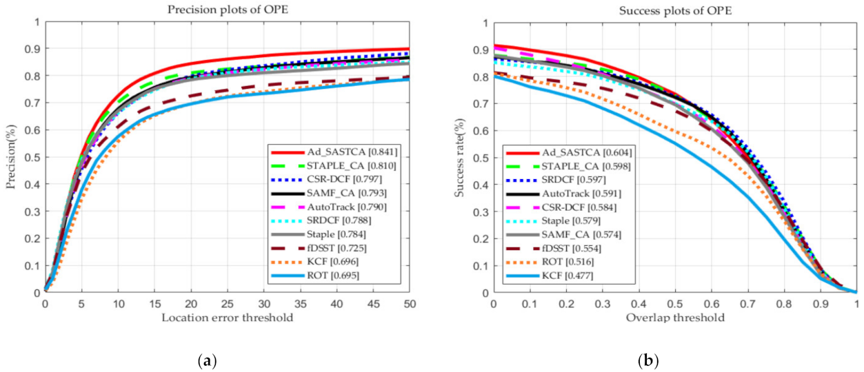
4.3.2. The OTB-2015 Benchmark

As Figure 4 shows, the overall performance of our proposed tracker is superior to the other 11 state-of-the-art trackers. Compared to the baseline tracker, Ad_SASTCA tracker improved the precision rate by 4.8% and the AUC score by 3%. In addition, in terms of both precision and AUC score, our proposed tracker provides a gain of 3.1% and 0.6% compared to ranked 2 STAPLE_CA method.

For completeness, we reported the accuracy of all trackers at a threshold of 20 pixels, as well as the tracking average speed in

Table 2. Precision rates (% at CLE = 20 pixs) of our proposed Ad_SASTCA versus other state-of-the-art trackers on OTB-2013 and OTB-2015. The best method is indicated in red, and the second and third are indicated in blue and green, respectively.

	Ours	STAPLE_CA	AutoTrack	CSR_DCF	Staple	SRDCF	SAMF_CA	fDSST	ROT	KCF
OTB-2013	85.9	83.2	83.0	80.3	78.2	83.8	80.3	80.3	74.4	74.0
OTB-2015	84.1	81.0	79.0	79.7	78.4	78.8	79.3	72.5	69.5	69.6
Avg.FPS	26.87	61.69	32.22	13.2	112.03	9.89	26.87	39.68	62.00	413.42

. The KCF tracker has the fastest tracking speed at 413.42 frames per second, followed by Staple (112.03 FPS) and ROT (62 FPS). The tracking speed of our tracker is over 25 FPS, reaching 26.87 FPS. This allows our proposed approach to be applied in scenarios with real-time applications.

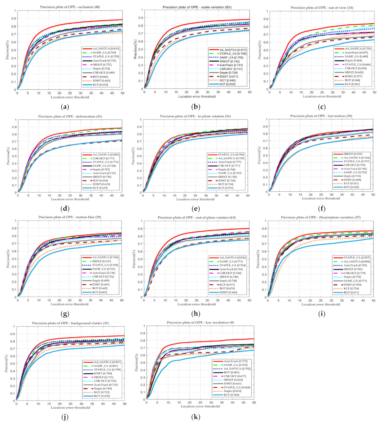
4.4. Attributes Based Evaluation and Discussion

Figure 5 illustrates the precision of the attribute-based evaluation performed on the OTB-2015 datasets for all CF-based trackers. The precision rate of each tracker for each attribute is indicated in square brackets. The experimental results indicate that among the 11 challenge attributes of the OTB datasets, our proposed Ad_SASTCA approach is superior to other DCF-based trackers in seven attributes, which are occlusion, scale variation, out-of-plane rotation, deformation, out-of-view, background clutter and motion blur. In addition, our tracker ranks second in illumination variation, fast motion and in-plane rotation attributes.

The experimental results suggest that, compared with the baseline SAMF_CA, the proposed approach achieves significant improvements in the two attributes of out-of-plane rotation and background clutter, with accuracy gains of 6.5% and 3.6%, respectively. Our high-confidence updating component and model persistent unreliability handling mechanism also lead to improvements in tracking performance. Compared with ROT, which has an occlusion-handling mechanism, our method provides a gain of 18.7% and 14.9% in the case of out-of-view and occlusion, respectively. In addition, all trackers utilized a comparison scale adaptive scheme except for KCF. Ad_SASTCA obtains a significant improvement of 14.6% over fDSST, which is designed specifically to handle scale changes. This indicates that the SAMF_CA scale estimation strategy is not just incorporated into our tracker, which can effectively handle the scale change of the object, because we introduce adaptive temporal regularization and background constraint in filter construction. As for the deformation attribute, Ad_SASTCA achieves a 3.2% improvement upon CSR-DCF. In particular, our proposed tracker obtains 2.8% gains over its baseline SAMF_CA tracker on the motion blur attribute.

4.5. The Qualitative Analysis and Discussion

For qualitative analysis and discussion, we compared our proposed approach with four state-of-the-art trackers, STAPLE_CA [28], SRDCF [26], CSR-DCF [32] and AutoTrack [34]. Figure 6 illustrates the results on eight video sequences in the OTB-2015 datasets, where each sequence may have several different challenges. Benefiting from our adaptive tracking strategy and the handling mechanism when the model is continuously unreliable. The target on the girls2 sequence undergoes long-term severe occlusion (approximately 16 frames) and out-of-view. Other trackers lost the target while our tracker never caused model drift throughout. A similar situation also appears in the lemming and Bird1 video sequences, where the Ad-SASTCA tracker is one of only two to re-capture the object when it disappears from the camera for a long period of time. Meanwhile, in the video sequences Board and jogging1, with significant deformations and shaking sequences with out-of-plane rotation attributes, our tracker can track the target very well. This is mainly attributed to the adaptive temporal regularization constraints. In addition, our tracker can effectively handle scale variations, such as the Human 3 sequences; however, we notice from sequence Bird1 that our tracker could not accurately estimate the scale change of the target when the target moved rapidly. However, such defects did not affect our tracker’s overall performance. Specifically, the Ad-SASTCA tracker is expert in solving out-of-view and occlusion (girl2, lemming, bird1), out-of-plane rotation (Shaking), significant deformation (jogging1, Board) and scale variation (Human3) scenarios.

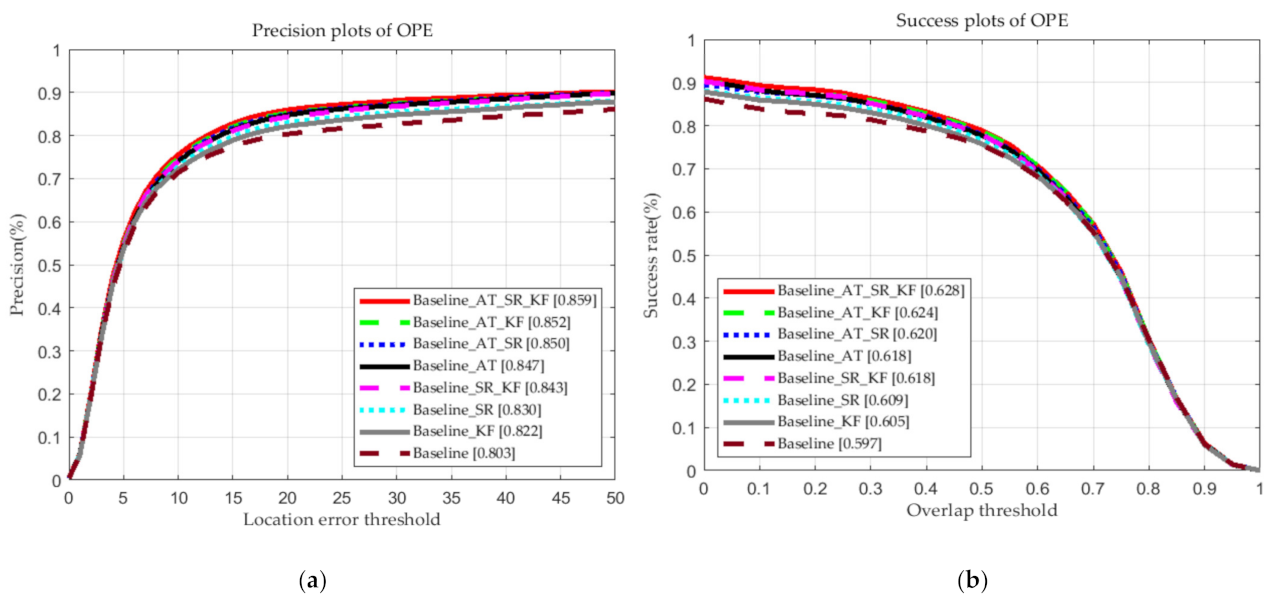
4.6. Ablation Studies and Discussion

To further validate the effectiveness of our proposed method, ablation studies are conducted on the OTB-2013 benchmark to evaluate the contribution of each incremental part, that is, the Kalman filter module (KF), adaptive temporal (AT) constraint and sparse response (SR) constraint in Equation (8). The baseline tracker is SAMF_CA, which is equipped with similar features as our method. The overall results are illustrated in Figure 7. With each component and their combinations added to the Baseline, the tracking performance is smoothly improved. Compared with the Baseline, the adaptive temporal constraint (Baseline_AT) and sparse response constraint (Baseline_SR) improved precision by 4.4% and 2.7%, respectively. The combination of two regularization constraints achieves (Baseline_AT_SR) a performance gain from 80.3% to 84.9% in precision and from 59.7% to 61.8% in AUC scores. Intuitively, the adaptive temporal constraint enables the learned filter to obtain a more robust appearance model, and the sparse response constraint reduces the risk of model drift. The combination of each regularization constraint and Kalman filter module also led to improvements in the tracking performance. Compared with Baseline_SR, the Kalman filter module (Baseline_SR_KF) improves the tracking performance in terms of precision and AUC by 1.3% and 0.9%, respectively. The introduction of the KF module also improves the tracking performance of the Baseline_AT tracker. Note that the KF module enables when the appearance model is unreliable persistently and abnormality occurs. The gains from the KF module are not as high as the regularization constraint. However, the KF module still improves the tracking performance. This shows that our multimodal tracking is effective. Because we did not contaminate the appearance model, thus, the model drift is avoided. In addition, the combination of all incremental parts is precisely the proposed Ad_SASTCA tracker, which achieved the best performance compared with the other combinations. The above results demonstrate the effectiveness of the proposed Ad_SASTCA.

4.7. The VOT2018 Benchmark

We evaluate our approach with 6 participating trackers on the VOT2018 benchmark, which contains 60 challenging video sequences. These trackers include SAMF_CA [28], KCF [21], DSST [43], SRDCF [26], STAPLE [45] and CSR_DCF [32]. We employ three metrics to evaluate the tracking performance: measures accuracy (A), robustness (R) and expected average overlap (EAO). The accuracy is the average overlap over successfully tracked frames. The robustness measures the average number of tracking failures during tracking. Furthermore, the EAO averages the no-reset overlap of a tracker on several short-term sequences.

Table 3. A comparison with the state-of-the-art trackers on VOT-2018 dataset. The best method is shown in red, and the second and third are shown in blue and green, respectively.

Tracker	Our	CSR_DCF	Staple	SAMF_CA	SRDCF	DSST	KCF
Accuracy	0.5122	0.4728	0.5035	0.4881	0.4634	0.3849	0.4394
Robustness	39.9532	24.9102	45.3015	52.3152	66.8433	96.7834	50.9617
EAO	0.1825	0.2503	0.1621	0.1490	0.1134	0.0780	0.1347

shows the results of the mentioned metrics. We can see from Table 3 that our proposed method performs better than other state-of-the-art trackers in terms of accuracy metrics. As for the robustness and EAO metric, CSR_DCF generates the highest EAO and robustness of 0.2503 and 24.9102, respectively, and our Ad_SASTCA obtains second place of the robustness and EAO. Overall, the results on the VOT2018 dataset show that our Ad_SASTCA can achieve better tracking performance.

5. Conclusions

In this study, a novel anti-drift object tracking algorithm was proposed, which not only considers the target’s temporal and spatial information, but also the sparse and local-global response variation. Moreover, we established a high-confidence update strategy and self-adapting learning rate based on the APCE-pool and Peak-pool. According to the evaluation results, we chose the CF tracker or the Kalman filter for target tracking to effectively avoid model drift. Finally, we compared the proposed Ad_SASTCA tracker with other state-of-the-art trackers on well-known benchmarks OTB-2013, OTB-2015 and VOT2018, for qualitative and quantitative evaluation. The experimental results showed that our tracker obtains remarkable performance.

Owing to the high precision and real-time performance of the proposed tracker, the Ad_SASTCA method can be successfully used in the field of autonomous driving and intelligent video monitoring applications. In the future, we will further improve our proposed tracker on several aspects, such as scale estimation, feature representation (such as deep CNN features) and model parameters optimization while ensuring real-time performance.

References

1. Cao, J.; Song, C.; Song, S.; Xiao, F.; Zhang, X.; Liu, Z.; Ang, M.H., Jr. Robust Object Tracking Algorithm for Autonomous Vehicles in Complex Scenes. Remote Sens. 2021, 13, 3234. [Google Scholar] [CrossRef]
2. Balamuralidhar, N.; Tilon, S.; Nex, F. MultEYE: Monitoring System for Real-Time Vehicle Detection, Tracking and Speed Estimation from UAV Imagery on Edge-Computing Platforms. Remote Sens. 2021, 13, 573. [Google Scholar] [CrossRef]
3. Chen, L.; Zhao, Y.; Yao, J.; Chen, J.; Li, N.; Chan, J.C.-W.; Kong, S.G. Object Tracking in Hyperspectral-Oriented Video with Fast Spatial-Spectral Features. Remote Sens. 2021, 13, 1922. [Google Scholar] [CrossRef]
4. Agarkhed, J.; Kulkarni, A.; Hiroli, N.; Kulkarni, J.; Jagde, A.; Pukale, A. Human Computer Interaction System Using Eye-Tracking Features. In Proceedings of the IEEE Bangalore Humanitarian Technology Conference (B-HTC), Vijiyapur, India, 8–10 October 2020; pp. 1–5. [Google Scholar]
5. Wei, H.; Huang, Y.; Hu, F.; Zhao, B.; Guo, Z.; Zhang, R. Motion Estimation Using Region-Level Segmentation and Extended Kalman Filter for Autonomous Driving. Remote Sens. 2021, 13, 1828. [Google Scholar] [CrossRef]
6. Wu, J.; Cao, C.; Zhou, Y.; Zeng, X.; Feng, Z.; Wu, Q.; Huang, Z. Multiple Ship Tracking in Remote Sensing Images Using Deep Learning. Remote Sens. 2021, 13, 3601. [Google Scholar] [CrossRef]
7. Wu, Y.; Lim, J.; Yang, M.H. Object tracking benchmark. IEEE Trans. Pattern Anal. Mach. Intell. 2015, 37, 1834–1848. [Google Scholar] [CrossRef] [Green Version]
8. Wu, Y.; Lim, J.; Yang, M.H. Online Object Tracking: A benchmark. In Proceedings of the IEEE Conference on Computer Vision and Pattern Recognition, Portland, OR, USA, 23–28 June 2013; pp. 2411–2418. [Google Scholar]
9. Zhang, T.; Bernard, G.; Liu, S.; Narendra, A. Robust Visual Tracking via Multi-Task Sparse Learning. In Proceedings of the IEEE Conference on Computer Vision and Pattern Recognition (CVPR), Providence, RI, USA, 16–21 June 2012; pp. 2042–2049. [Google Scholar]
10. Zhang, T.; Xu, C.; Yang, M. Robust Structural Sparse Tracking. IEEE Trans. Pattern Anal. Mach. Intell. 2019, 41, 473–486. [Google Scholar] [CrossRef]
11. Wang, Q.; Chen, F.; Xu, W.; Yang, M. Object Tracking via Partial Least Squares Analysis. IEEE Trans. Image Process. 2012, 21, 4454–4465. [Google Scholar] [CrossRef] [Green Version]
12. Zhang, Y.; Wang, T.; Liu, K.; Zhang, B.; Chen, L. Recent advances of single-object tracking methods: A brief survey. Neurocomputing 2021, 455, 1–11. [Google Scholar] [CrossRef]
13. Babenko, B.; Yang, M.; Belongie, S. Robust Object Tracking with Online Multiple Instance Learning. IEEE Trans. Pattern Anal. Mach. Intell. 2012, 13, 1619–1632. [Google Scholar] [CrossRef] [Green Version]
14. Ma, B.; Shen, J.; Liu, Y.; Hu, H.; Shao, L.; Li, X. Visual Tracking Using Strong Classifier and Structural Local Sparse Descriptors. IEEE Trans. Multimed. 2015, 17, 1818–1828. [Google Scholar] [CrossRef]
15. Zhang, S.; Yu, X.; Sui, Y.; Zhao, S.; Zhang, L. Object Tracking with Multi-View Support Vector Machines. IEEE Trans. Multimed. 2015, 17, 265–278. [Google Scholar] [CrossRef]
16. Hare, S.; Golodetz, S.; Saffari, A.; Vineet, V.; Cheng, M.M.; Hicks, S.L.; Torr, P.H.S. Struck: Structured output tracking with kernels. IEEE Trans. Pattern Anal. 2016, 38, 2096–2109. [Google Scholar] [CrossRef] [PubMed] [Green Version]
17. Dinh, T.B.; Vo, N.; Medioni, G. Context tracker: Exploring Supporters and Distracters in Unconstrained Environments. In Proceedings of the 2011 IEEE Conference on Computer Vision and Pattern Recognition (CVPR), Colorado Springs, CO, USA, 20–25 June 2011; pp. 1177–1184. [Google Scholar]
18. Jiang, N.; Liu, W.Y.; Wu, Y. Learning adaptive metric for robust visual tracking. IEEE Trans. Image Process. 2011, 20, 2288–2300. [Google Scholar] [CrossRef]
19. Bolme, D.S.; Beveridge, J.R.; Draper, B.A.; Lui, Y.M. Visual Object Tracking Using Adaptive Correlation Filters. In Proceedings of the IEEE Conference on Computer Vision and Pattern Recognition, San Francisco, CA, USA, 13–18 June 2010; pp. 2544–2550. [Google Scholar]
20. Henriques, J.F.; Caseiro, R.; Martins, P.; Batista, J. Exploiting the circulant structure of tracking-by-detection with kernels. Lect. Notes Comput. Sci. 2012, 7575, 702–715. [Google Scholar]
21. Henriques, J.F.; Caseiro, R.; Martins, P.; Batista, J. High-speed tracking with kernelized correlation filters. IEEE Trans. Pattern Anal. Mach. Intell. 2014, 37, 583–596. [Google Scholar] [CrossRef] [Green Version]
22. Nam, H.; Han, B. Learning Multi-Domain Convolutional Neural Networks for Visual Tracking. In Proceedings of the 29th IEEE Conference on Computer Vision and Pattern Recognition (CVPR), Las Vegas, NV, USA, 26 June–1 July 2016; pp. 4293–4302. [Google Scholar]
23. Zhu, K.; Zhang, X.; Chen, G.; Tan, X.; Liao, P.; Wu, H.; Cui, X.; Zuo, Y.; Lv, Z. Single object tracking in satellite videos: Deep Siamese network incorporating an interframe difference centroid inertia motion model. Remote Sens. 2021, 13, 1298. [Google Scholar] [CrossRef]
24. Huang, B.; Xu, T.; Shen, Z.; Jiang, S.; Zhao, B.; Bian, Z. SiamATL: Online Update of Siamese Tracking Network via Attentional Transfer Learning. IEEE Trans. Cybern. 2021. [Google Scholar] [CrossRef] [PubMed]
25. Kristan, M.; Leonardis, A.; Matas, J. The Sixth Visual Object Tracking vot2018 Challenge Results. In Proceedings of the European Conference on Computer Vision (ECCV), Munich, Germany, 8–14 September 2018. [Google Scholar]
26. Danelljan, M.; Häger, G.; Khan, F.S.; Felsberg, M. Learning Spatially Regularized Correlation Filters for Visual Tracking. In Proceedings of the IEEE International Conference on Computer Vision (ICCV), Santiago, Chile, 7–13 December 2015; pp. 4310–4318. [Google Scholar]
27. Li, F.; Tian, C.; Zuo, W.; Zhang, L.; Yang, M.H. Learning Spatial-temporal Regularized Correlation Filters for Visual Tracking. In Proceedings of the IEEE Conference on Computer Vision and Pattern Recognition, Salt Lake City, UT, USA, 19–21 June 2018; pp. 4904–4913. [Google Scholar]
28. Mueller, M.; Smith, N.; Ghanem, B. Context-Aware Correlation Filter Tracking. In Proceedings of the IEEE Conference on Computer Vision and Pattern Recognition (CVPR), Honolulu, HI, USA, 21–26 July 2017; pp. 1387–1395. [Google Scholar]
29. Danelljan, M.; Robinson, A.; Khan, F.S.; Felsberg, M. Beyond Correlation Filters: Learning Continuous Convolution Operators for Visual Tracking. In Proceedings of the European Conference on Computer Vision, Amsterdam, The Netherlands, 8–16 October 2016; pp. 472–488. [Google Scholar]
30. Danelljan, M.; Bhat, G.; Shahbaz Khan, F.; Felsberg, M. Eco: Efficient Convolution Operators for Tracking. In Proceedings of the IEEE Conference on Computer Vision and Pattern Recognition, Honolulu, HI, USA, 22–25 July 2017; pp. 6638–6646. [Google Scholar]
31. Kiani Galoogahi, H.; Fagg, A.; Lucey, S. Learning Background-aware Correlation Filters for Visual Tracking. In Proceedings of the IEEE International Conference on Computer Vision, Venice, Italy, 19–22 October 2017; pp. 1135–1143. [Google Scholar]
32. Lukežic, A.; Vojír, T.; Zajc, L.C.; Matas, J.; Kristan, M. Discriminative Correlation Filter with Channel and Spatial Reliability. In Proceedings of the IEEE Conference on Computer Vision and Pattern Recognition (CVPR), Honolulu, HI, USA, 21–26 July 2017; pp. 4847–4856. [Google Scholar]
33. Elayaperumal, D.; Joo, Y.H. Aberrance suppressed spatio-temporal correlation filters for visual object tracking. Pattern Recognit. 2021, 115, 107922. [Google Scholar] [CrossRef]
34. Li, Y.; Fu, C.; Ding, F.; Huang, Z.; Lu, G. AutoTrack: Towards High-Performance Visual Tracking for UAV With Automatic Spatio-Temporal Regularization. In Proceedings of the IEEE/CVF Conference on Computer Vision and Pattern Recognition (CVPR), Seattle, WA, USA, 13–19 June 2020; pp. 11920–11929. [Google Scholar]
35. Han, Y.; Deng, C.; Zhao, B.; Zhao, B. Spatial-Temporal Context-Aware Tracking. IEEE Signal Process. Lett. 2019, 26, 500–504. [Google Scholar] [CrossRef]
36. Wang, M.; Liu, Y.; Huang, Z. Margin Object Tracking with Circulant Feature Maps. In Proceedings of the IEEE Conference on Computer Vision and Pattern Recognition, Honolulu, HI, USA, 21–26 July 2017; pp. 4800–4808. [Google Scholar]
37. Dong, X.; Shen, J.; Yu, D.; Wang, W.; Liu, J.; Huang, H. Occlusion-Aware Real-Time Object Tracking. IEEE Trans. Multimed. 2017, 19, 763–771. [Google Scholar] [CrossRef]
38. Han, Y.; Deng, C.; Zhao, B.; Tao, D. State-Aware Anti-Drift Object Tracking. IEEE Trans. Image Process. 2019, 28, 4075–4086. [Google Scholar] [CrossRef] [Green Version]
39. Du, S.; Wang, S. An Overview of Correlation-Filter-Based Object Tracking. IEEE Trans. Comput. Soc. Syst. 2021, 1–14. [Google Scholar] [CrossRef]
40. Dalal, N.; Triggs, B. Histograms of Oriented Gradients for Human Detection. In Proceedings of the IEEE Computer Society Conference on Computer Vision and Pattern Recognition (CVPR’05), San Diego, CA, USA, 20–25 June 2005; pp. 886–893. [Google Scholar]
41. Danelljan, M.; Shahbaz Khan, F.; Felsberg, M.; Van de Weijer, J. Adaptive Color Attributes for Real-time Visual Tracking. In Proceedings of the IEEE Conference on Computer Vision and Pattern Recognition, Columbus, OH, USA, 24–27 June 2014; pp. 1090–1097. [Google Scholar]
42. Li, Y.; Zhu, J. A Scale Adaptive Kernel Correlation Filter Tracker with Feature Integration. In Proceedings of the European Conference on Computer Vision, Zurich, Switzerland, 5–12 September 2014; pp. 254–265. [Google Scholar]
43. Danelljan, M.; Häger, G.; Khan, F.S.; Felsberg, M. Accurate Scale Estimation for Robust Visual Tracking. In Proceedings of the British Machine Vision Conference, Nottingham, UK, 1–5 September 2014. [Google Scholar]
44. Danelljan, M.; Häger, G.; Khan, F.S.; Felsberg, M. Discriminative Scale Space Tracking. IEEE Trans. Pattern Anal. Mach. Intell. 2017, 39, 8. [Google Scholar] [CrossRef] [Green Version]
45. Bertinetto, L.; Valmadre, J.; Golodetz, S.; Miksik, O.; Torr, P.H. Staple: Complementary Learners for Real-time Tracking. In Proceedings of the IEEE Conference on Computer Vision and Pattern Recognition, Las Vegas, NV, USA, 26 June–1 July 2016; pp. 1401–1409. [Google Scholar]
46. Kalal, Z.; Mikolajczyk, K.; Matas, J. Tracking-learning-detection. IEEE Trans. Pattern Anal. Mach. Intell. 2012, 34, 1409–1422. [Google Scholar] [CrossRef] [PubMed] [Green Version]
47. Ma, C.; Yang, X.; Zhang, C.; Yang, M. Long-Term Correlation Tracking. In Proceedings of the 2015 IEEE Conference on Computer Vision and Pattern Recognition (CVPR), Boston, MA, USA, 7–12 June 2015; pp. 5388–5396. [Google Scholar]
48. Cheng, J.; Tsai, Y.; Hung, W.; Wang, S.; Yang, M. Fast and Accurate Online Video Object Segmentation via Tracking Parts. In Proceedings of the IEEE/CVF Conference on Computer Vision and Pattern Recognition, Salt Lake City, UT, USA, 18–23 June 2018; pp. 7415–7424. [Google Scholar]
49. Bhat, G.; Danelljan, M.; Gool, L.; Timofte, R. Learning Discriminative Model Prediction for Tracking. In Proceedings of the IEEE/CVF International Conference on Computer Vision (ICCV), Seoul, Korea, 27 October–2 November 2019; pp. 6181–6190. [Google Scholar]
50. Valmadre, J.; Bertinetto, L.; Henriques, J.; Vedaldi, A.; Torr, P.H.S. End-to-End Representation Learning for Correlation Filter Based Tracking. In Proceedings of the IEEE Conference on Computer Vision and Pattern Recognition (CVPR), Honolulu, HI, USA, 21–26 July 2017; pp. 5000–5008. [Google Scholar]
51. Wang, Q.; Zhang, L.; Bertinetto, L.; Hu, W.; Torr, P.H.S. Fast Online Object Tracking and Segmentation: A Unifying Approach. In Proceedings of the IEEE/CVF Conference on Computer Vision and Pattern Recognition (CVPR), Long Beach, CA, USA, 15–20 June 2019; pp. 1328–1338. [Google Scholar]
52. Voigtlaender, P.; Luiten, J.; Torr, P.H.S.; Leibe, B. Siam R-CNN: Visual Tracking by Re-Detection. In Proceedings of the IEEE/CVF Conference on Computer Vision and Pattern Recognition (CVPR), Seattle, WA, USA, 13–19 June 2020; pp. 6577–6587. [Google Scholar]
53. Boyd, S.; Parikh, E.; Chu, E.; Peleato, B.; Eckstein, J. Distributed Optimization and Statistical Learning via the Alternating Direction Method of Multipliers. Found. Trends Mach. Learn. 2011, 3, 1–122. [Google Scholar] [CrossRef]
54. Huang, B.; Xu, T.; Jiang, S.; Chen, Y.; Bai, Y. Robust Visual Tracking via Constrained Multi-Kernel Correlation Filters. IEEE Trans. Multimed. 2020, 22, 2820–2832. [Google Scholar] [CrossRef]
Figure 1. Flow chart of the Ad_SASTCA framework.
Remotesensing 13 04672 g001
Figure 2. The APCE and peak normalized change curve of our Ad_SASTCA model on the sequence “Liquor” from 1200 frame to 1380 frame. Severe occlusion in frames 1237, 1287, 1230 and 1356 nearby will lead the APCE and peak of response to dropping sharply in a short period. Because the Ad_SASTCA does not fuse excessive incorrect information into the appearance model, the response map still indicates a sharp unimodal peak, and the model drift is avoided.
Remotesensing 13 04672 g002
Figure 3. Overall experimental results of precision plot (a) and success plot (b) comparing Ad_SASTCA with nine state-of the art trackers on OTB-2013. The trackers in figures (a) and (b) are sorted according to precision and AUCs, respectively. Best viewed in color and high resolution.
Remotesensing 13 04672 g003
Figure 4. Overall results of precision plot (a) and success plot (b) comparing Ad_SASTCA with nine state-of the art trackers on OTB-2015 dataset. The trackers in figures (a) and (b) are sorted according to precision and AUCs, respectively.
Remotesensing 13 04672 g004
Figure 5. Attribute based evaluation. Precision plots (ak) are indicated on the OTB-2015 dataset for 11 challenge attributes. Precision rates are reported in brackets. The title of each plot includes the number of videos related attributes.
Remotesensing 13 04672 g005
Figure 6. Illustration of qualitative tracking results on challenging sequences (From top to bottom: (a) lemming, (b) BlurOwl, (c) Girl2, (d) Bird1, (e) Shaking, (f) Board, (g) Human2 and (h) Human3). The colour bounding boxes are the corresponding results of Ad_SASTCA, STAPLE_CA [28], CSR_DCF [32], SRDCF [26] and AutoTrack [34].
Remotesensing 13 04672 g006aRemotesensing 13 04672 g006b
Figure 7. The performance of different components and their combinations in Ad_SASTCA, evaluated on OTB-2013. The trackers in figures (a) and (b) are sorted according to precision and AUCs, respectively.
Remotesensing 13 04672 g007