
A Sentinel-1 Backscatter Datacube for Global Land Monitoring Applications †

 , , , , , ,
  and
and
Abstract
:
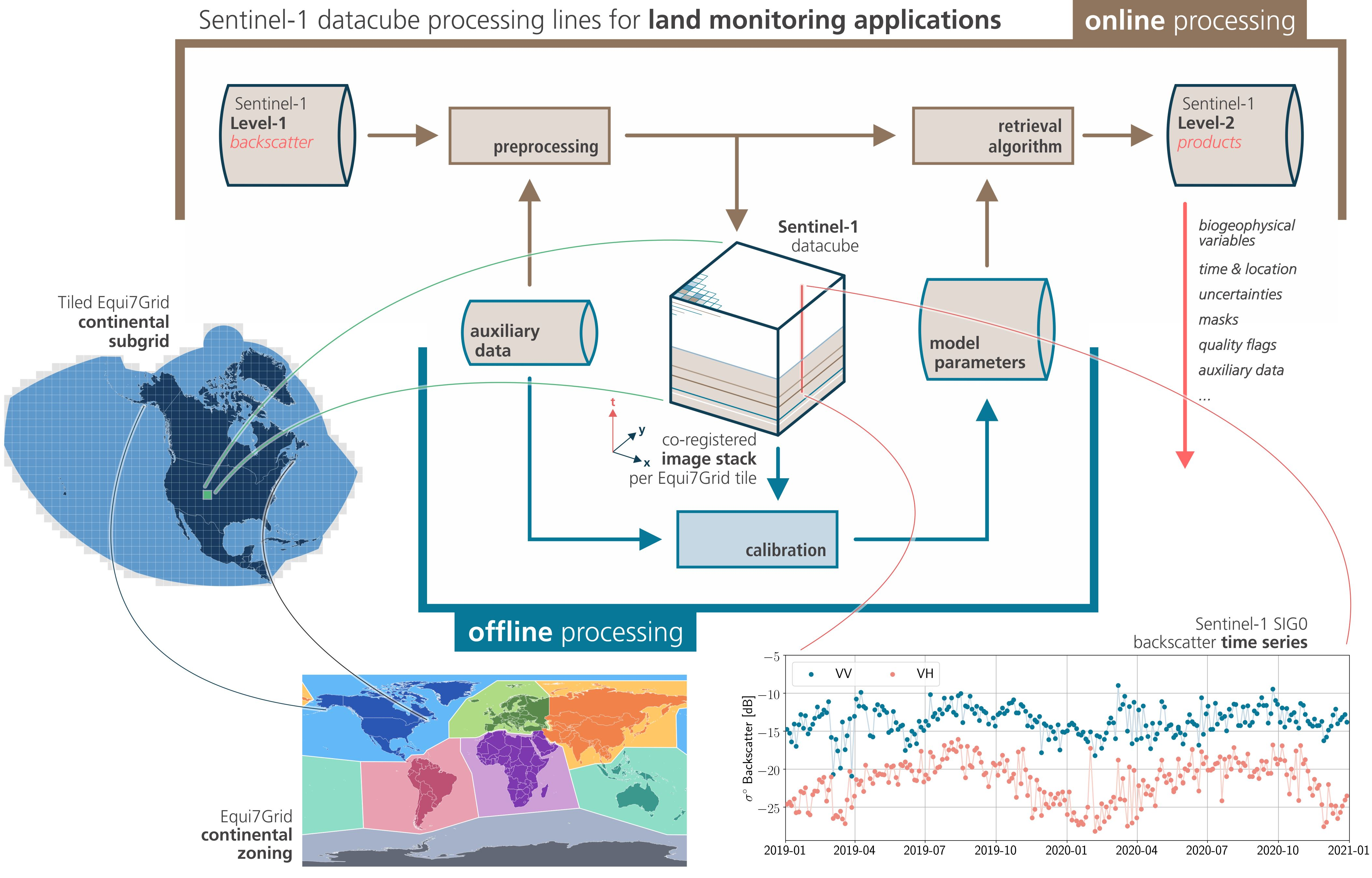
1. Introduction
- The datacube represents a complete collection of Sentinel-1 data over land surfaces and covers all continents except Antarctica;
- The system enables both offline analyses of multi-year time series and near-real-time image-based applications;
- There should be maximum flexibility regarding the type of scientific algorithms to be deployed on the data;
- It shall be accessible and usable for a large number of users with different backgrounds and interests;
- Reprocessing of the complete petabyte-scale data collection must be possible to ensure that the data are consistent and comply with the latest processing standards.
2. Materials and Methods
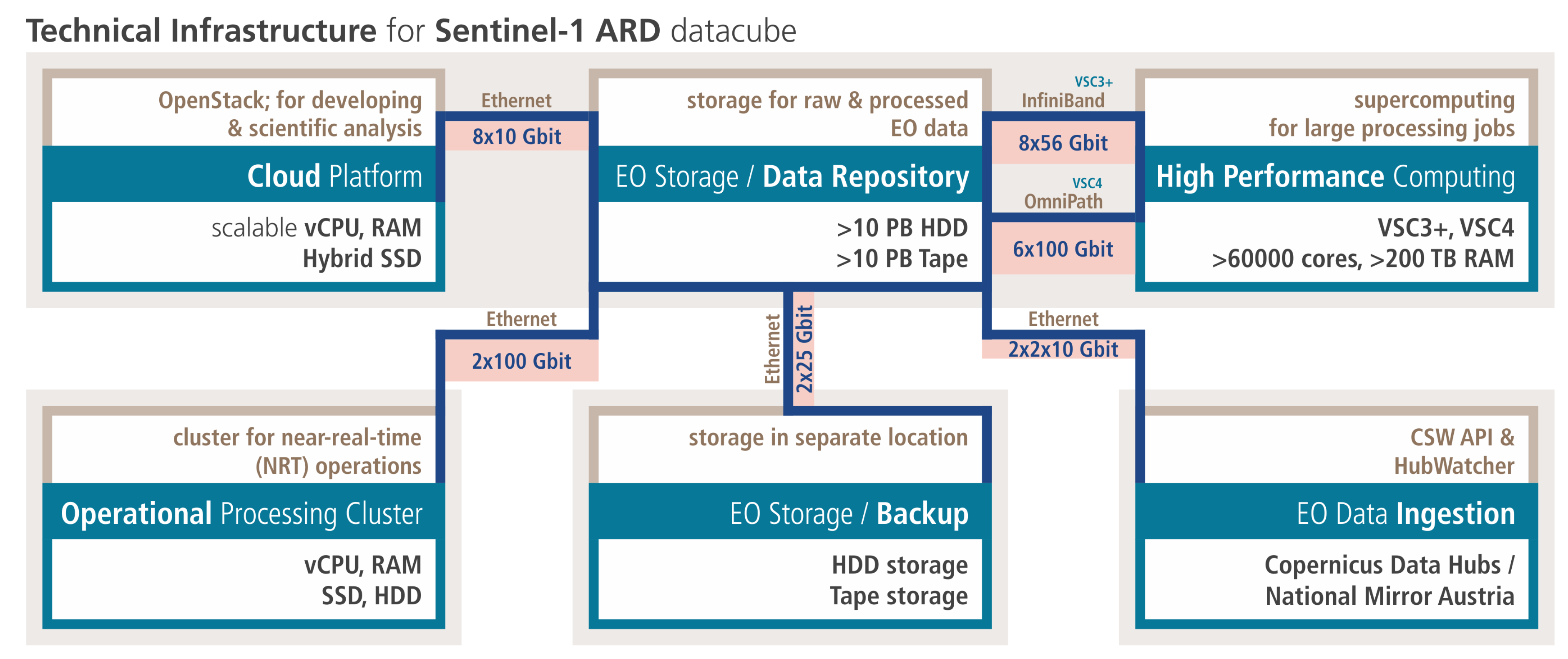
2.1. Cloud Infrastructure
- Cloud Platform [11]: The cloud platform is based on the open-source cloud software OpenStack [12]. Users can request and setup virtual machines (VMs) according to their needs (virtual CPUs, RAM, hybrid-SSD storage, open-source software) and directly access the global Sentinel-1 backscatter datacube along with the other datasets hosted in the EODC data repository (Sentinel-2 Level-1C, etc.). This environment is particularly suited for scientific analysis, code development, and testing. Larger processing jobs, involving e.g., the analysis of the entire Sentinel-1 period for a few tiles, are possible. Nonetheless, for very large processing activities, e.g., covering bigger countries or whole continents, moving to supercomputers may be necessary.
- High-Performance Computing (HPC) [13]: Thanks to dedicated high-throughput I/O connections (InfiniBand and OmniPath), it is possible to process the Sentinel-1 data on one of the HPC-clusters of the Vienna Scientific Cluster (VSC) facility. Normally, two supercomputers are operational at the same time. So far, Sentinel-1 data processing has taken place using the oil-cooled VSC-3 cluster and its air-cooled VSC-3+ extension. At present, Sentinel-1 processing is being moved to the VSC-4, the current flagship that reaches a performance of 2.7 PFlop/s with its 790 water-cooled nodes. The EODC storage can be accessed from VSC in the same logic, but with less visualisation/development functions than on the cloud platform. The benefit is that processing of Sentinel-1 images at hundreds of compute nodes in parallel is possible. Nonetheless, tailoring of the processing routines to balance I/O, storage, and compute resources is usually required.
- Operational Processing Cluster: This dedicated cluster serves operational near-real-time (NRT) applications and is used for fully automatic updating of the global datacube as soon as new Sentinel-1 images become available.
2.2. Sentinel-1 Data
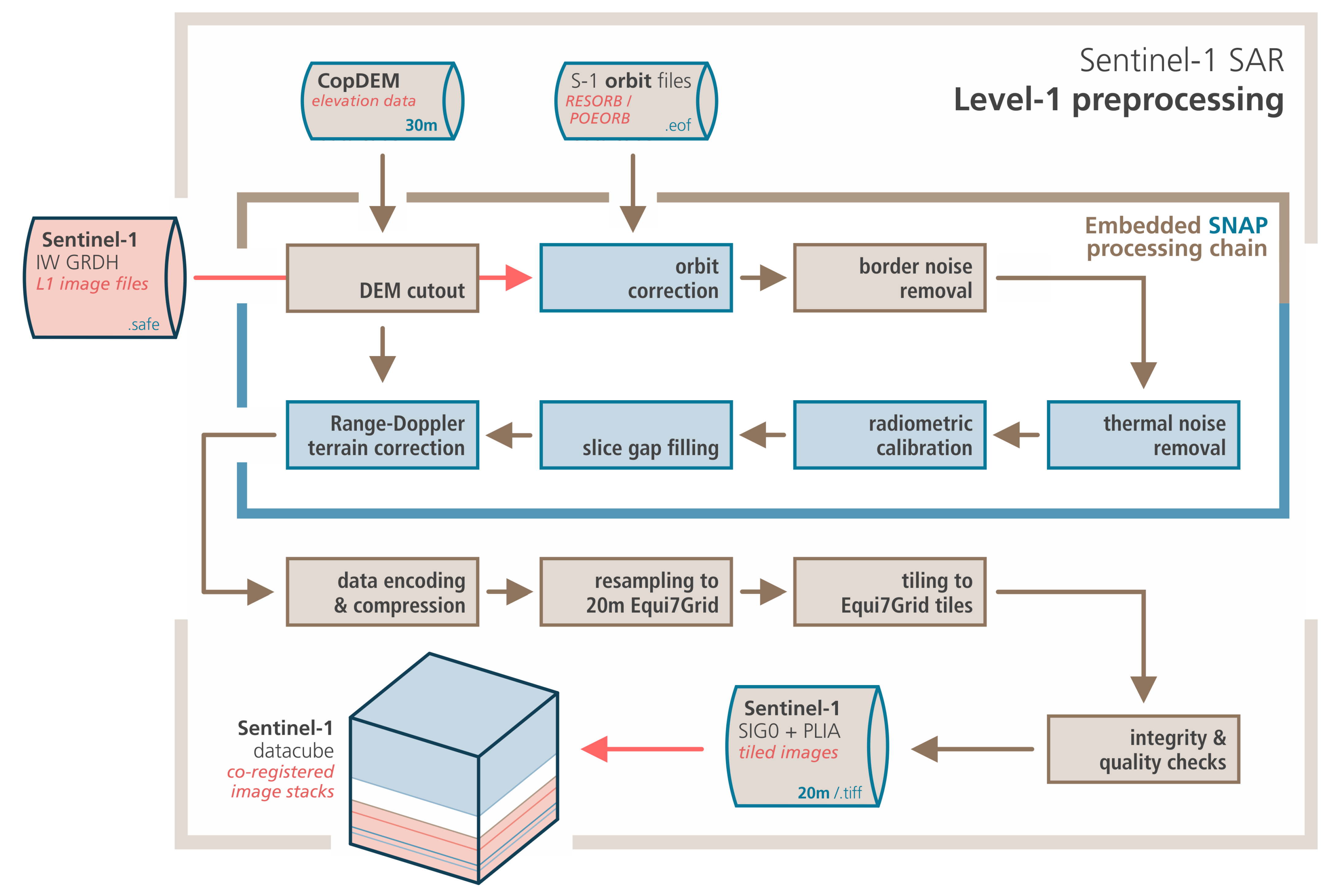
2.3. Data Preparation
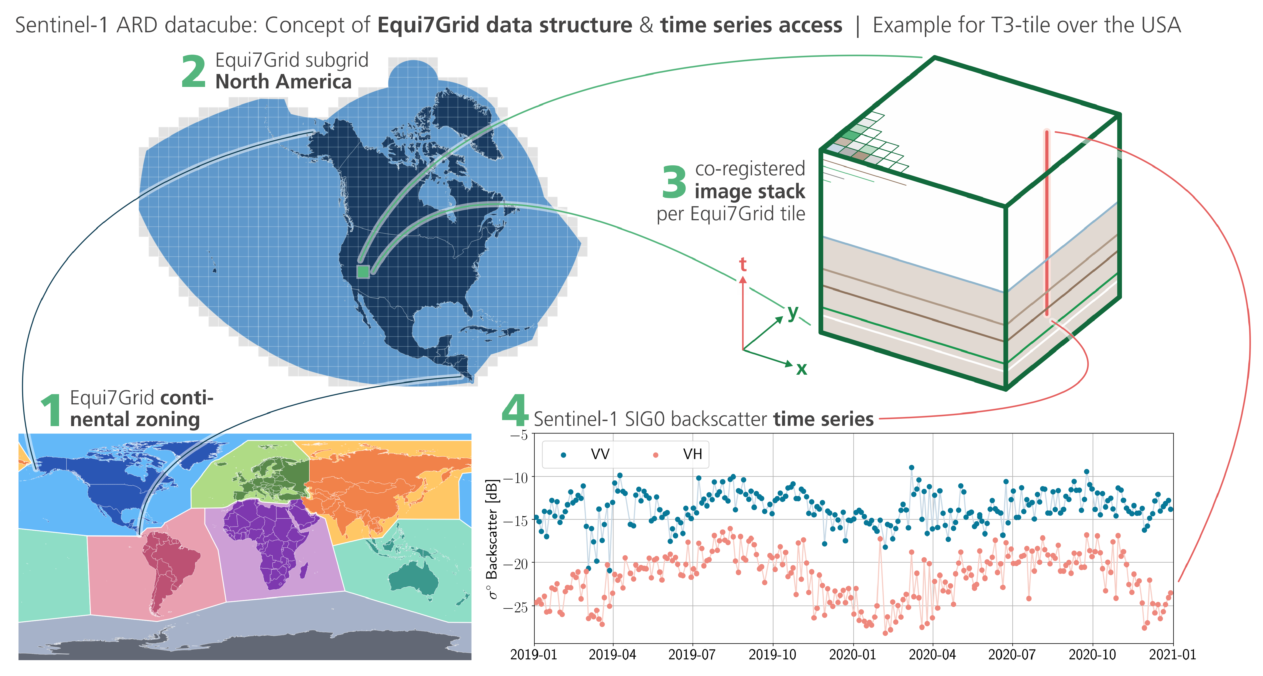
3. Datacube
3.1. Production
3.2. Technical Specifications
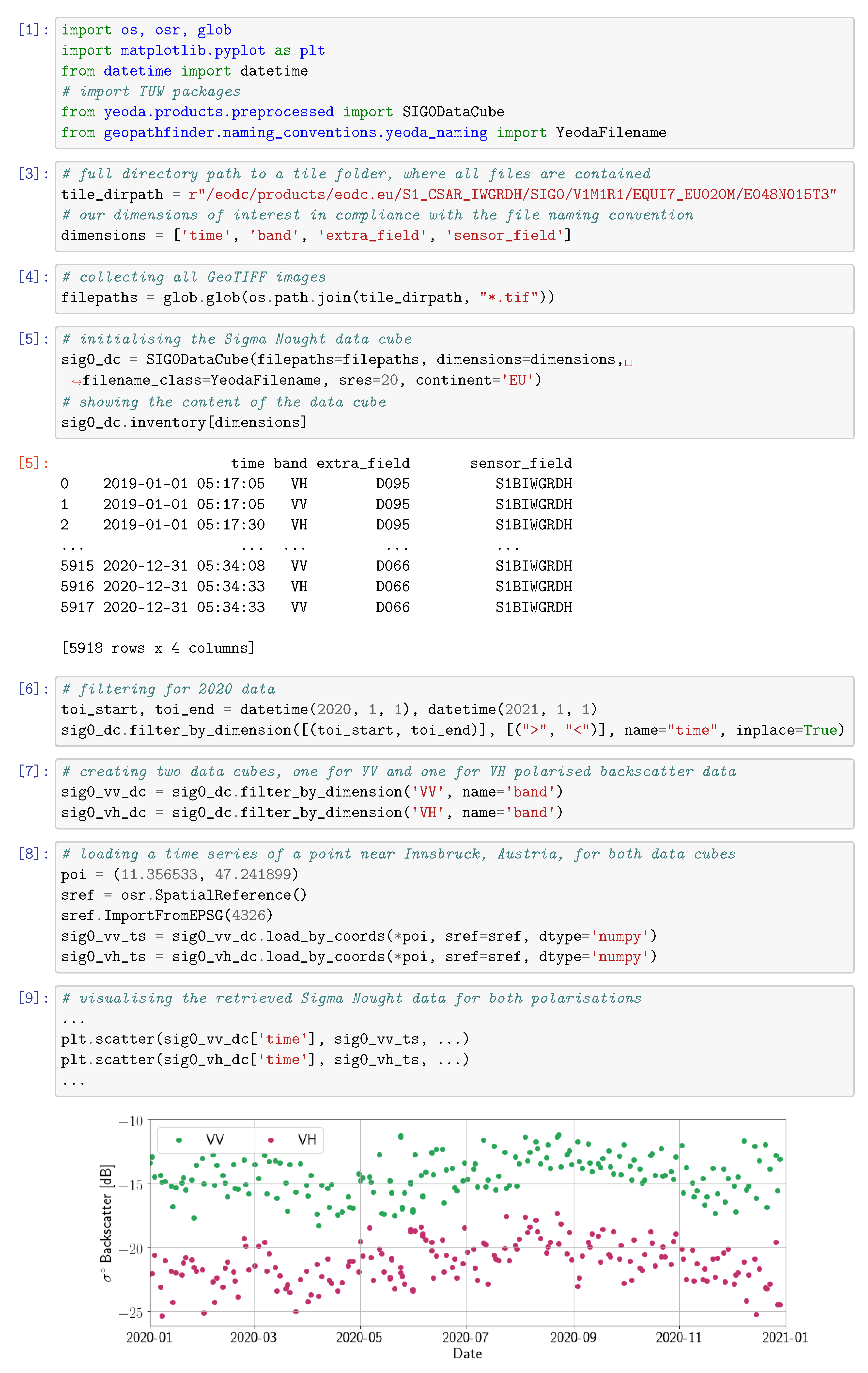
3.3. Access
- datacube instances may persist in memory for consecutive access
- it will be possible to jointly load data beyond the tile boundaries of the Equi7Grid
- more efficient data management in the background
- coupling of datacubes to a database for more performant queries, mimicking Open Data Cube’s software architecture
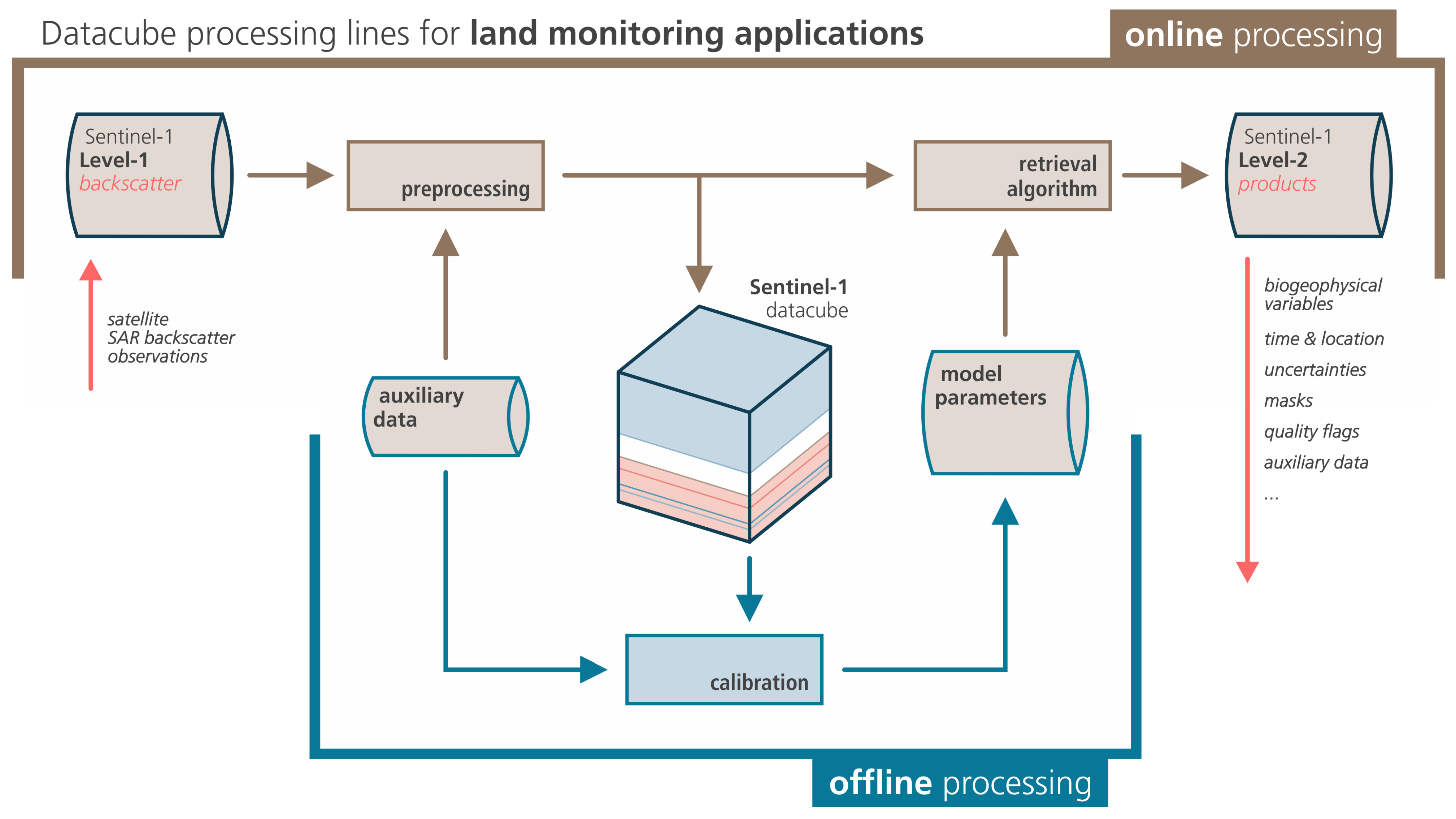
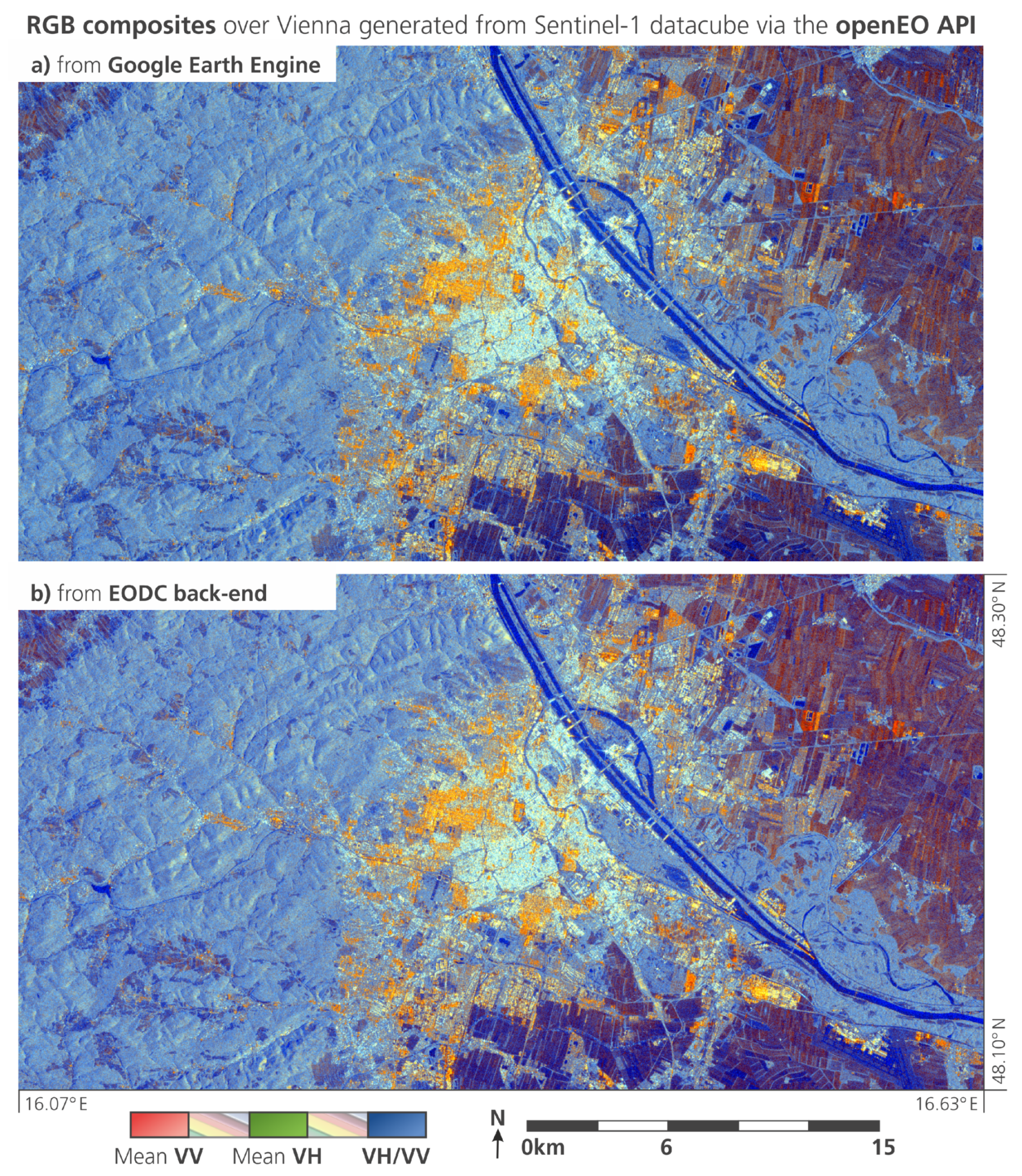
3.4. Applications
4. Discussion
5. Conclusions
Funding
Data Availability Statement
Acknowledgments
Conflicts of Interest
Abbreviations
| API | Application Programming Interface |
| ARD | Analysis Ready Data |
| CEOS | Committee of Earth Observation Satellites |
| CGLS | Copernicus Global Land Service |
| CSW | Catalogue Service for the Web |
| DEM | Digital Elevation Model |
| DIAS | Data and Information Access Service |
| EGM | Earth Gravitational Model |
| EO | Earth Observation |
| EODC | Earth Observation Data Centre for Water Resources Monitoring |
| EGM | Earth Gravitational Model |
| ESA | European Space Agency |
| GEE | Google Earth Engine |
| GFM | Global Flood Monitoring |
| GPF | Graph Processing Framework |
| GRD | Ground Range Detected |
| HDD | Hard Disk Drive |
| HPC | High Performance Computing |
| IW | Sentinel-1 Interferometric Wide-Swath Mode |
| I/O | Input/Output |
| NRT | Near Real Time |
| POEORB | Precise Orbit files |
| POD | Precise Orbit Determination |
| RESORB | Restituted Orbit files |
| RGB | Red-Green-Blue |
| SAR | Synthetic Aperture Radar |
| SNAP | Sentinel Application Platform |
| SLC | Single Look Complex |
| SRTM | Shuttle Radar Topography Mission |
| SSD | Solid State Disk |
| UTM | Universal Transversal Mercator projection |
| VM | Virtual Machine |
| VSC | Vienna Scientific Cluster |
References
- Torres, R.; Snoeij, P.; Geudtner, D.; Bibby, D.; Davidson, M.; Attema, E.; Potin, P.; Rommen, B.; Floury, N.; Brown, M.; et al. GMES Sentinel-1 mission. Remote Sens. Environ. 2012, 120, 9–24. [Google Scholar] [CrossRef]
- Thompson, A.A. Overview of the RADARSAT Constellation Mission. Can. J. Remote Sens. 2015, 41, 401–407. [Google Scholar] [CrossRef]
- Woodhouse, I.H. Introduction to Microwave Remote Sensing; CRC Press: Boca Raton, FL, USA, 2017. [Google Scholar] [CrossRef]
- Gao, Q.; Zribi, M.; Escorihuela, M.; Baghdadi, N.; Segui, P. Irrigation Mapping Using Sentinel-1 Time Series at Field Scale. Remote Sens. 2018, 10, 1495. [Google Scholar] [CrossRef] [Green Version]
- Schlund, M.; Erasmi, S. Sentinel-1 time series data for monitoring the phenology of winter wheat. Remote Sens. Environ. 2020, 246, 111814. [Google Scholar] [CrossRef]
- Dostálová, A.; Lang, M.; Ivanovs, J.; Waser, L.T.; Wagner, W. European Wide Forest Classification Based on Sentinel-1 Data. Remote Sens. 2021, 13, 337. [Google Scholar] [CrossRef]
- Kopp, S.; Becker, P.; Doshi, A.; Wright, D.J.; Zhang, K.; Xu, H. Achieving the Full Vision of Earth Observation Data Cubes. Data 2019, 4, 94. [Google Scholar] [CrossRef] [Green Version]
- Gorelick, N.; Hancher, M.; Dixon, M.; Ilyushchenko, S.; Thau, D.; Moore, R. Google Earth Engine: Planetary-scale geospatial analysis for everyone. Remote Sens. Environ. 2017, 202, 18–27. [Google Scholar] [CrossRef]
- Wagner, W.; Bauer-Marschallinger, B.; Navacchi, C.; Reuss, F.; Cao, S.; Reimer, C.; Schramm, M.; Briese, C. A Sentinel-1 Data Cube For Global Land Monitoring Applications. In Proceedings of the 2021 Conference on Big Data from Space (BiDS’21), Online Conference, 18–20 May 2021; Publications Office of the European Union: Luxembourg, 2021; pp. 49–52. [Google Scholar] [CrossRef]
- Wagner, W.; Fröhlich, J.; Wotawa, G.; Stowasser, R.; Staudinger, M.; Hoffmann, C.; Walli, A.; Federspiel, C.; Aspetsberger, M.; Atzberger, C.; et al. Addressing Grand Challenges in Earth Observation Science: The Earth Observation Data Centre for Water Resources Monitoring. ISPRS Ann. Photogramm. Remote Sens. Spatial Inf. Sci. 2014, II-7, 81–88. [Google Scholar] [CrossRef] [Green Version]
- EODC. EODC Cloud. Available online: https://eodc.eu/services/cloud (accessed on 22 September 2021).
- OpenStack. Available online: https://www.openstack.org/ (accessed on 29 September 2021).
- EODC. High Performance Computing. Available online: https://eodc.eu/services/hpc (accessed on 22 September 2021).
- Ticehurst, C.; Zhou, Z.S.; Lehmann, E.; Yuan, F.; Thankappan, M.; Rosenqvist, A.; Lewis, B.; Paget, M. Building a SAR-Enabled Data Cube Capability in Australia Using SAR Analysis Ready Data. Data 2019, 4, 100. [Google Scholar] [CrossRef] [Green Version]
- Knowelden, R.; Castriotta, A.G. Copernicus Sentinel Data Access—2019 Annual Report. 2020. Available online: https://sentinels.copernicus.eu/web/sentinel/news/-/asset_publisher/xR9e/content/copernicus-sentinel-data-access-annual-report-2019;jsessionid=4DC08B0ABC1B60CB9A889CD1AF2B53B1.jvm2?redirect=https%3A%2F%2Fsentinels.copernicus.eu%2Fweb%2Fsentinel%2Fnews%3Bjsessionid%3D4DC08B0ABC1B60CB9A889CD1AF2B53B1.jvm2%3Fp_p_id%3D101_INSTANCE_xR9e%26p_p_lifecycle%3D0%26p_p_state%3Dnormal%26p_p_mode%3Dview%26p_p_col_id%3Dcolumn-1%26p_p_col_count%3D1%26_101_INSTANCE_xR9e_keywords%3D%26_101_INSTANCE_xR9e_advancedSearch%3Dfalse%26_101_INSTANCE_xR9e_delta%3D20%26_101_INSTANCE_xR9e_andOperator%3Dtrue (accessed on 22 September 2021).
- SkyWatch; German Aerospace Center (DLR); Brockmann Consult; OceanDataLab. Sentinel-1 Toolbox. 2021. Available online: https://step.esa.int/main/toolboxes/sentinel-1-toolbox/ (accessed on 29 September 2021).
- OSGeo. GDAL. Available online: https://gdal.org/ (accessed on 27 September 2021).
- Anaconda. Numba. Available online: http://numba.pydata.org/ (accessed on 27 September 2021).
- Truckenbrodt, J.; Freemantle, T.; Williams, C.; Jones, T.; Small, D.; Dubois, C.; Thiel, C.; Rossi, C.; Syriou, A.; Giuliani, G. Towards Sentinel-1 SAR Analysis-Ready Data: A Best Practices Assessment on Preparing Backscatter Data for the Cube. Data 2019, 4, 93. [Google Scholar] [CrossRef] [Green Version]
- Small, D. Flattening Gamma: Radiometric Terrain Correction for SAR Imagery. IEEE Trans. Geosci. Remote Sens. 2011, 49, 3081–3093. [Google Scholar] [CrossRef]
- Small, D.; Rohner, C.; Miranda, N.; Rüetschi, M.; Schaepman, M.E. Wide-Area Analysis-Ready Radar Backscatter Composites. IEEE Trans. Geosci. Remote Sens. 2021, 1–14. [Google Scholar] [CrossRef]
- Bruggisser, M.; Dorigo, W.; Dostálová, A.; Hollaus, M.; Navacchi, C.; Schlaffer, S.; Pfeifer, N. Potential of Sentinel-1 C-Band Time Series to Derive Structural Parameters of Temperate Deciduous Forests. Remote Sens. 2021, 13, 798. [Google Scholar] [CrossRef]
- Fahrland, E. Copernicus Digital Elevation Model Product Handbook, Version 2.1; Airbus, 2020. Available online: https://spacedata.copernicus.eu/documents/20126/0/GEO1988-CopernicusDEM-SPE-002_ProductHandbook_I1.00.pdf (accessed on 16 November 2021).
- Peters, M. Creating a GPF Graph. Available online: https://senbox.atlassian.net/wiki/spaces/SNAP/pages/70503590/Creating+a+GPF+Graph (accessed on 29 September 2021).
- Ali, I.; Cao, S.; Naeimi, V.; Paulik, C.; Wagner, W. Methods to Remove the Border Noise From Sentinel-1 Synthetic Aperture Radar Data: Implications and Importance For Time-Series Analysis. IEEE J. Sel. Top. Appl. Earth Observ. Remote Sens. 2018, 11, 777–786. [Google Scholar] [CrossRef] [Green Version]
- Bauer-Marschallinger, B.; Sabel, D.; Wagner, W. Optimisation of global grids for high-resolution remote sensing data. Comput. Geosci. 2014, 72, 84–93. [Google Scholar] [CrossRef]
- Amatulli, G.; McInerney, D.; Sethi, T.; Strobl, P.; Domisch, S. Geomorpho90m, empirical evaluation and accuracy assessment of global high-resolution geomorphometric layers. Sci. Data 2020, 7, 162. [Google Scholar] [CrossRef]
- Roy, D.P.; Li, J.; Zhang, H.K.; Yan, L. Best practices for the reprojection and resampling of Sentinel-2 Multi Spectral Instrument Level 1C data. Remote Sens. Lett. 2016, 7, 1023–1032. [Google Scholar]
- TU Wien GEO Department. Equi7Grid—GitHub. Available online: https://github.com/TUW-GEO/Equi7Grid (accessed on 22 September 2021).
- Elefante, S.; Wagner, W.; Briese, C.; Cao, S.; Naeimi, V. High-performance computing for soil moisture estimation. In Proceedings of the 2016 Conference on Big Data from Space (BiDS’16), Santa Cruz de Tenerife, Spain, 15–17 March 2016; Publications Office of the European Union: Santa Cruz de Tenerife, Spain, 2016; pp. 95–98. [Google Scholar] [CrossRef]
- Ali, I.; Naeimi, V.; Cao, S.; Elefante, S.; Le, T.; Bauer-Marschallinger, B.; Wagner, W. Sentinel-1 data cube exploitation: Tools, products, services and quality control. In Proceedings of the 2017 Conference on Big Data from Space (BiDS’17), Toulouse, France, 28–30 November 2017; Publications Office of the European Union: Toulouse, France, 2016; pp. 40–43. [Google Scholar] [CrossRef]
- Copernicus-ESA. The Copernicus Services Data Hub. Available online: https://colhub.copernicus.eu/ (accessed on 27 September 2021).
- Copernicus-ESA. The Sentinels Collaborative Data Hub. Available online: https://colhub.copernicus.eu/ (accessed on 27 September 2021).
- EODC. CSW. Available online: https://eodc.eu/services/pycsw (accessed on 22 September 2021).
- TU Wien GEO Department. yeoda—GitHub. Available online: https://github.com/TUW-GEO/yeoda (accessed on 22 September 2021).
- ODC. Open Data Cube. Available online: https://www.opendatacube.org/ (accessed on 22 September 2021).
- Killough, B. Overview of the Open Data Cube Initiative. In Proceedings of the IGARSS 2018—2018 IEEE International Geoscience and Remote Sensing Symposium, Valencia, Spain, 22–27 July 2018; pp. 8629–8632. [Google Scholar] [CrossRef]
- TU Wien GEO Department. yeoda—Read the Docs. Available online: https://yeoda.readthedocs.io/en/latest/index.html (accessed on 22 September 2021).
- Nguyen, D.B.; Wagner, W. European Rice Cropland Mapping with Sentinel-1 Data: The Mediterranean Region Case Study. Water 2017, 9, 392. [Google Scholar] [CrossRef]
- Vreugdenhil, M.; Navacchi, C.; Bauer-Marschallinger, B.; Hahn, S.; Steele-Dunne, S.; Pfeil, I.; Dorigo, W.; Wagner, W. Sentinel-1 Cross Ratio and Vegetation Optical Depth: A Comparison over Europe. Remote Sens. 2020, 12, 3404. [Google Scholar] [CrossRef]
- Bauer-Marschallinger, B.; Freeman, V.; Cao, S.; Paulik, C.; Schaufler, S.; Stachl, T.; Modanesi, S.; Massari, C.; Ciabatta, L.; Brocca, L.; et al. Toward Global Soil Moisture Monitoring With Sentinel-1: Harnessing Assets and Overcoming Obstacles. IEEE Trans. Geosci. Remote Sens. 2019, 57, 520–539. [Google Scholar] [CrossRef]
- Frantz, D.; Schug, F.; Okujeni, A.; Navacchi, C.; Wagner, W.; van der Linden, S.; Hostert, P. National-scale mapping of building height using Sentinel-1 and Sentinel-2 time series. Remote Sens. Environ. 2021, 252, 112128. [Google Scholar] [CrossRef] [PubMed]
- Bauer-Marschallinger, B.; Cao, S.; Navacchi, C.; Freeman, V.; Reuß, F.; Geudtner, D.; Rommen, B.; Ceba Vega, F.; Snoeij, P.; Attema, E.; et al. The normalised Sentinel-1 Global Backscatter Model, mapping Earth’s land surface with C-band microwaves. Sci. Data 2021, 8, 277. [Google Scholar] [CrossRef] [PubMed]
- Copernicus Programme. Copernicus Land Monitoring Service. Available online: https://land.copernicus.eu/ (accessed on 21 September 2021).
- Copernicus Programme. Copernicus Emergency Management Service. Available online: https://emergency.copernicus.eu/ (accessed on 21 September 2021).
- Li, Y.; Martinis, S.; Plank, S.; Ludwig, R. An automatic change detection approach for rapid flood mapping in Sentinel-1 SAR data. Int. J. Appl. Earth Observ. Geoinf. 2018, 73, 123–135. [Google Scholar] [CrossRef]
- Lievens, H.; Demuzere, M.; Marshall, H.P.; Reichle, R.H.; Brucker, L.; Brangers, I.; de Rosnay, P.; Dumont, M.; Girotto, M.; Immerzeel, W.W.; et al. Snow depth variability in the Northern Hemisphere mountains observed from space. Nat. Commun. 2019, 10, 4629. [Google Scholar] [CrossRef]
- El Hajj, M.; Baghdadi, N.; Wigneron, J.P.; Zribi, M.; Albergel, C.; Calvet, J.C.; Fayad, I. First Vegetation Optical Depth Mapping from Sentinel-1 C-band SAR Data over Crop Fields. Remote Sens. 2019, 11, 2769. [Google Scholar] [CrossRef] [Green Version]
- Balenzano, A.; Mattia, F.; Satalino, G.; Lovergine, F.P.; Palmisano, D.; Peng, J.; Marzahn, P.; Wegmüller, U.; Cartus, O.; Dąbrowska-Zielińska, K.; et al. Sentinel-1 soil moisture at 1 km resolution: A validation study. Remote Sens. Environ. 2021, 263, 112554. [Google Scholar] [CrossRef]
- Matgen, P.; Martinis, S.; Wagner, W.; Freeman, V.; Zeil, P.; McCormick, N. Feasibility Assessment of an Automated, Global, Satellite-Based Flood Monitoring Product for the Copernicus Emergency Management Service; Technical Report JRC116163; European Commission Joint Research Centre: Ispra, Italy, 2019. [Google Scholar]
- Wagner, W.; Freeman, V.; Cao, S.; Matgen, P.; Chini, M.; Salamon, P.; McCormick, N.; Martinis, S.; Bauer-Marschallinger, B.; Navacchi, C.; et al. Data processing architectures for monitoring floods using Sentinel-1. ISPRS Ann. Photogramm. Remote Sens. Spatial Inf. Sci. 2020, V-3-2020, 641–648. [Google Scholar] [CrossRef]
- Rasdaman. Available online: http://www.rasdaman.org/ (accessed on 27 September 2021).
- Baumann, P.; Misev, D.; Merticariu, V.; Huu, B.P.; Bell, B. rasdaman: Spatio-temporal datacubes on steroids. In Proceedings of the 26th ACM SIGSPATIAL International Conference on Advances in Geographic Information Systems, Seattle, WA, USA, 6–9 November 2018; pp. 604–607. [Google Scholar] [CrossRef]
- Project Jupyter. JupyterHub. Available online: https://jupyter.org/hub (accessed on 27 September 2021).
- OSGeo. GeoServer. Available online: http://geoserver.org/ (accessed on 27 September 2021).
- EODC. Austrian Data Cube. Available online: https://acube.eodc.eu/ (accessed on 27 September 2021).
- Schramm, M.; Pebesma, E.; Milenković, M.; Foresta, L.; Dries, J.; Jacob, A.; Wagner, W.; Mohr, M.; Neteler, M.; Kadunc, M.; et al. The openEO API–Harmonising the Use of Earth Observation Cloud Services Using Virtual Data Cube Functionalities. Remote Sens. 2021, 13, 1125. [Google Scholar] [CrossRef]
- Mullissa, A.; Vollrath, A.; Odongo-Braun, C.; Slagter, B.; Balling, J.; Gou, Y.; Gorelick, N.; Reiche, J. Sentinel-1 SAR Backscatter Analysis Ready Data Preparation in Google Earth Engine. Remote Sens. 2021, 13, 1954. [Google Scholar] [CrossRef]
- Canty, M.J.; Nielsen, A.A.; Conradsen, K.; Skriver, H. Statistical Analysis of Changes in Sentinel-1 Time Series on the Google Earth Engine. Remote Sens. 2020, 12, 46. [Google Scholar] [CrossRef] [Green Version]
- Greifeneder, F.; Notarnicola, C.; Wagner, W. A Machine Learning-Based Approach for Surface Soil Moisture Estimations with Google Earth Engine. Remote Sens. 2021, 13, 2099. [Google Scholar] [CrossRef]
- Committee on Earth Observation Satellites. CEOS Analysis Ready Data. Available online: https://ceos.org/ard/ (accessed on 22 September 2021).
- European Space Agency. openEO Platform. Available online: https://docs.openeo.cloud/ (accessed on 22 September 2021).
- Copernicus. Copernicus and Sentinel Data at your Fingertips. Available online: https://www.wekeo.eu/ (accessed on 22 September 2021).


| Level-1 Sentinel-1 IW GRD Data | |||||||
| Year | Africa | Asia | Europe | NA | Oceania | SA | Total |
| 2015 | 12.7 | 15.1 | 22.0 | 6.2 | 4.9 | 5.3 | 66.2 |
| 2016 | 20.6 | 19.2 | 31.9 | 11.5 | 6.6 | 9.0 | 98.8 |
| 2017 | 45.0 | 53.9 | 71.8 | 31.4 | 18.4 | 23.1 | 243.6 |
| 2018 | 48.0 | 58.1 | 70.3 | 35.3 | 20.2 | 24.7 | 256.6 |
| 2019 | 94.4 | 61.1 | 119.9 | 38.5 | 21.1 | 26.9 | 361.9 |
| 2020 | 97.3 | 63.3 | 130.7 | 41.4 | 21.3 | 28.6 | 382.6 |
| Total | 318.0 | 270.7 | 446.6 | 164.3 | 92.5 | 117.6 | 1409.7 |
| 20 m Sentinel-1 Datacube | |||||||
| Year | Africa | Asia | Europe | NA | Oceania | SA | Total |
| 2015 | 2.5 | 2.9 | 4.3 | 1.2 | 1.1 | 1.0 | 13.0 |
| 2016 | 4.4 | 4.0 | 6.4 | 2.5 | 1.5 | 1.9 | 20.7 |
| 2017 | 9.8 | 11.9 | 14.6 | 6.9 | 4.3 | 4.9 | 52.4 |
| 2018 | 10.3 | 12.8 | 12.8 | 7.6 | 4.7 | 5.2 | 53.4 |
| 2019 | 16.9 | 19.4 | 23.5 | 13.4 | 7.6 | 8.6 | 89.4 |
| 2020 | 17.3 | 20.1 | 25.0 | 14.6 | 7.7 | 9.4 | 94.1 |
| Total | 61.2 | 71.1 | 86.6 | 46.1 | 26.9 | 31.0 | 323.0 |
Publisher’s Note: MDPI stays neutral with regard to jurisdictional claims in published maps and institutional affiliations. |
© 2021 by the authors. Licensee MDPI, Basel, Switzerland. This article is an open access article distributed under the terms and conditions of the Creative Commons Attribution (CC BY) license (https://creativecommons.org/licenses/by/4.0/).
Share and Cite
Wagner, W.; Bauer-Marschallinger, B.; Navacchi, C.; Reuß, F.; Cao, S.; Reimer, C.; Schramm, M.; Briese, C. A Sentinel-1 Backscatter Datacube for Global Land Monitoring Applications. Remote Sens. 2021, 13, 4622. https://doi.org/10.3390/rs13224622
Wagner W, Bauer-Marschallinger B, Navacchi C, Reuß F, Cao S, Reimer C, Schramm M, Briese C. A Sentinel-1 Backscatter Datacube for Global Land Monitoring Applications. Remote Sensing. 2021; 13(22):4622. https://doi.org/10.3390/rs13224622
Chicago/Turabian StyleWagner, Wolfgang, Bernhard Bauer-Marschallinger, Claudio Navacchi, Felix Reuß, Senmao Cao, Christoph Reimer, Matthias Schramm, and Christian Briese. 2021. "A Sentinel-1 Backscatter Datacube for Global Land Monitoring Applications" Remote Sensing 13, no. 22: 4622. https://doi.org/10.3390/rs13224622