Article

Dynamic Object Detection Algorithm Based on Lightweight Shared Feature Pyramid

1
National Key Laboratory of Science and Technology on Multi-Spectral Information Processing, School of Artificial Intelligence and Automation, Huazhong University of Science and Technology, Wuhan 430074, China
2
School of Biomedical Engineering, South-Central University for Nationalities, Wuhan 430074, China
*
Author to whom correspondence should be addressed.
Remote Sens. 2021, 13(22), 4610; https://doi.org/10.3390/rs13224610
Submission received: 28 September 2021 / Revised: 10 November 2021 / Accepted: 12 November 2021 / Published: 16 November 2021
(This article belongs to the Special Issue UAV Photogrammetry for 3D Modeling)

Abstract

:
Current object detection algorithms perform inference on all samples at a fixed computational cost in the inference stage, which wastes computing resources and is not flexible. To solve this problem, a dynamic object detection algorithm based on a lightweight shared feature pyramid is proposed, which performs adaptive inference according to computing resources and the difficulty of samples, greatly improving the efficiency of inference. Specifically, a lightweight shared feature pyramid network and lightweight detection head is proposed to reduce the amount of computation and parameters in the feature fusion part and detection head of the dynamic object detection model. On the PASCAL VOC dataset, under the two conditions of “anytime prediction” and “budgeted batch object detection”, the performance, computation amount and parameter amount are better than the dynamic object detection models constructed by networks such as ResNet, DenseNet and MSDNet.

1. Introduction

Recent years have witnessed remarkable progress in object detection field thanks to the advance of the deep convolution networks [1,2,3,4]. However, the explosive growth in model size and computation cost gives rise to new challenges on how to efficiently deploy these deep learning models on resource-constrained devices while maintain the performance as much as possible. Nowadays, there have been many studies to accelerate the inference of deep models through lightweight network architecture design [5,6,7], weight quantization [8,9] and network pruning [10,11,12]. Compared to static models which have fixed computational graphs and parameters at the inference stage, dynamic neural networks [13,14,15,16,17] aim to reduce the computational redundancy on “easy” samples. By dynamically adjusting the network structure or parameters to different inputs, dynamic neural networks have been shown to have notable advantages in terms of accuracy and computational efficiency.
A straightforward implementation of dynamic network is performing inference with dynamic network depths, which can be realized by early exiting, i.e., allowing “easy” samples to be output at shallow exits without executing deeper layers. MSDNet [13], designed for image classification task, adopts (1) a multiscale architecture, which consists of multiple sub-networks for processing different scale feature maps, to quickly generate coarse-level features that are suitable for classification; (2) dense connections, reusing early features to improve the performance of deep classifiers. They consider two settings for this kind of network: one is “Anytime prediction”, the network’s prediction result of a test sample is gradually updated, so that it can stop inference at any time; the second setting is “Budgeted batch classification”. In this setting, the model needs to classify a set of examples within a finite computational budget B that is known in advance. These two settings are of great value in practical applications. For example, there are tens of thousands of mobile devices with different computing capabilities on the market. The “Anytime prediction” network can process videos on any device at a fixed frame rate, and according to the device to maximize the computing power performance, it is much easier than training networks of different sizes for different devices. “Batch classification with budget” can save computing resources by reducing the amount of inference calculations for simple samples.
However, due to the special structure of the object detection network, it is not trivial to extend the multiscale architecture to the object detection model. Table 1 shows the average computation and parameter amount of each image inferenced by MSDNet on the test set of the PASCAL VOC dataset. The unit of the computation amount statistics is GFlops (Giga Floating-Point Operations Per Second), that is, every second 1 billion floating point operations. It can be seen from the table that the total amount of computation of the entire feature extraction network is 28.4G, and the amount of parameters is 16.8M. Here we take RetinaNet [18] as an comparison. Its backbone network is ResNet-50. It has only a single detection head attached at the last stage feature maps of ResNet-50. It can be seen from Table 2 that most of the computation and parameters of the entire detection model are concentrated on the detection head. The calculation volume of a detection head is 54.5G and the parameter volume is 26.09M, which has far exceeded the amount of calculations and parameters of the entire feature extraction network of MSDNet. When constructing a dynamic model that has multiple detection heads attached at different stage of the deep network, a huge amount of computation and parameters will be generated. In addition, the computation volume of the FPN part is 8.5G, and the parameter volume is 8M. When it is expanded to multiple detection heads, the calculation volume and the parameter volume increase greatly. Therefore, to construct a dynamic object detection model with multiple detection heads, it is indispensable to improve the FPN and the detection head network.
We investigate the demand of object detection network for dynamic prediction structure. In this paper, based on MSDNet, we construct a new multiscale and dense connection structure for the object detector model, which can stop the prediction at any time according to the given computing power during the inference process and return the detection result. To solve the problem of the sharp increase of computation and parameters caused by the change of network structure, we propose a lightweight shared feature pyramid network in the multiscale feature fusion part of the dynamic object detection model. A lightweight detection head network is also designed to reduce calculation and parameters of the prediction head network. Extensive experiments on benchmark datasets show that the proposed method is theoretically reasonable and practically effective. On the PASCAL VOC dataset, under the two conditions of “anytime prediction” and “budgeted batch object detection”, the performance, calculation amount and parameter amount are better than the dynamic object detection models constructed by networks such as ResNet, DenseNet and MSDNet. The code is made publicly available at https://github.com/zl1994/DLSFPN, accessed on 27 September 2021.

2. Related Works

2.1. Object Detection Algorithm Based on Deep Learning

Nowadays, as the deep learning techniques have been widely applied to various computer vision tasks, convolution neural networks (CNNs)-based methods have prevailed in object detection task and the model architectures are constantly evolving. R-CNN [19] is the first CNN-based object detector. It uses region proposals to locate objects in images and region proposals are potential bounding boxes, which are generated by traditional region proposal methods [20,21]. Then, a convolution network extracts features of proposal and feeds these features into a subsequent network. After that, proposals are classified into foreground classes or background. At the same time, their locations are refined by bounding box regression. Finally, non-max suppression is used to eliminate duplicate bounding boxes and obtain the ultimate result. The derivatives of R-CNN, Fast R-CNN [22] and Faster R-CNN [23], further improve the speed and performance. Fast R-CNN introduced the RoI Pooling module and enabled end-to-end training. Faster R-CNN proposed a fully convolutional architecture, known as Region Proposal Network (RPN), for efficient and accurate region proposal generation. RPN replaces the time-consuming region proposal algorithms. The method described above and the following R-FCN [24] and Cascade R-CNN [25] can be classified into two-stage methods. Two-stage methods obtain a set of proposals in the first stage. Then they further classify and refine these proposals at the second stage. On the other hand, one-stage methods, popularized by YOLO [26,27] and SSD [28], were developed to directly predict bounding boxes and classification scores, without additional stage to generate proposals. YOLO-LITE [29] further proposed a light version of YOLO for real-time applications running on portable devices. Compared to two-stage methods, one-stage methods achieve high inference speed but the accuracy is worse. The performance gap between two-stage methods and one-stage methods was narrowed by RetinaNet [18]. It inherits the fast speed of previous one-stage methods while alleviate the extreme foreground–background class imbalance encountered during training. Sufficient data are the key to maintaining high performance of deep learning algorithms. In the case of lacking in infrared videos data, the authors of [30] apply the data generation methods based on generative adversarial network (GAN) models [31] to generate realistic infrared images from optical images and improve the object detection performance using real-infrared videos. As the one-stage and two-stage detection frameworks become mature, the anchor-free methods have led to a new research trend. Without using anchor boxes, they predict bounding boxes in a per-pixel prediction manner [32,33] or keypoint-based fashion [34,35]. In recent years, network architecture search (NAS)-based research has also been developed vigorously. EfficientDet [36] disassembles the modules with different layers of object detector and performs scaling on the image size and network layers. RegNet [37] uses six parameters to perform a compound model scaling search.

2.2. Feature Pyramids Based on Deep Learning

Feature pyramid networks (FPN) [38] builds a feature pyramid by combining two adjacent layers in feature hierarchy in backbone network with top-down and lateral connections. With the help of pyramid structure, the detectors enhance its feature extraction capabilities and further improving performance. Many follow-up studies extend the idea to build stronger feature pyramid representations. PANet [39] adds a bottom-up path relative to FPN to enhances the information propagation ability of feature pyramids. CARAFE [40] integrates an effective feature upsampling operators into FPN to boost the performance. NAS-FPN [41] adopts neural architecture search to find a new feature pyramid architecture. It indicates that fusing features from both top-down and bottom-up connections with different scales can increase detection accuracy by a large margin. Ref. [42] proposes a dynamic FPN to choose the proper kernel sizes of conv layers for different samples. Different from them, in this article, we focus on optimizing the structure of FPN to adapt to the multiscale architecture.

2.3. Dynamic Neural Networks

Dynamic neural network is one of the effective methods to reduce the amount of network computation. It can be adaptively adjusted to achieve real time on devices with different computing capabilities and can perform adaptive inference according to the difficulty of the sample, which effectively improves the efficiency of inference. Thanks to its attractive characteristics, the research direction is gaining increasing attention. The most intuitive implementation of dynamic structure is assembling multiple models and then selecting a subset of them to execute in a cascading [15] or mixing way [16]. Recent works also propose to selectively skip some layers or blocks [17,43,44], or adaptively select different channels [45] for different examples during inference. Refs. [46,47] attach multiple auxiliary predictors at different stage of the deep network. Thus, some “easy” examples can obtain results from the front predictor without routing the latter part of the network. Furthermore, CADDet [48] applies the dynamic routing strategy to activate part of the whole network for each sample. Previous work [49] suggested that not all locations contribute equally to the feature extraction and prediction of CNNs. To reduce the redundancy on less informative locations, some dynamic convolution methods [50,51] have been proposed to perform convolution only on sampled pixels.
In 2018, Huang et al. [13] proposed MSDNet, which has multiple classification heads and can be withdrawn at any time during the forward propagation process. MSDNet can choose whether to perform forward propagation according to the difficulty of the samples, thereby reducing the amount of calculation.The author defines two resource-constrained condition settings: one is “anytime prediction”; the other is “budgeted batch classification”, and proposes to verify under these two condition settings the performance of such algorithms. In 2020, Yang et al. [14] proposed RANet. The author conducted research from the perspective of network input size, and proposed a network that adaptively adjusts the input resolution. It sets a smaller input size for simple samples and a larger input size for difficult samples improves the efficiency of the inference stage. However, most of these prior works focus on designing adaptive networks for image classification task and it is not suitable for the dynamic neural network on the object detection model. Different from the previous dynamic networks, we extend the idea of MSDNet and first introduce a suitable multilayer prediction method of dynamic neural network for current detection model.

3. Method

In this section, we first introduce the overall network architecture and the adaptive inference settings of the dynamic object detection model. Then we demonstrate the details of the feature extraction network, lightweight shared feature pyramid network and lightweight detection head network, respectively.

3.1. Adaptive Inference Settings

The adaptive inference model is an object detection network with multiple detection heads, which are connected to feature maps of different depths of the backbone. For the input picture x, the output of the prediction result of the k-th detection head is formalized as:
P k = f k x ; θ k = P 1 k , , P n k T R n L k = f k x ; θ k = L 1 k , , L n k T R n P n k = max P n 1 k , P n 2 k , , P n c k
where θ k represents the parameters of the k-th detection head, P n k [ 0 , 1 ] represents the maximum value of the confidence of the c categories predicted by the n-th prediction boxes after non-maximum suppression, L n k represents the predicted coordinates of the n-th prediction frame after nonmaximum suppression, and some parameters of θ k are shared.
The adaptive inference model can adaptively allocate computing resources according to the complexity of the sample. When the output of the detection head meets a specific criterion for the first time, the sample will exit the inference and return the result. In our paper, we use the highest confidence of the softmax output as the criterion. When the highest confidence level of the softmax output of all prediction boxes is greater than a given threshold ϵ for the first time greater than N, the model stops inference and returns the results of the current detection head:
k = min k n P n k ε > N y ^ P k , L k , ( a ) = 0 , a < 0 1 , a 0
y ^ denotes the predictions of the k-th detection head. ϵ controls the balance of performance and computation cost, and N is set to 4.

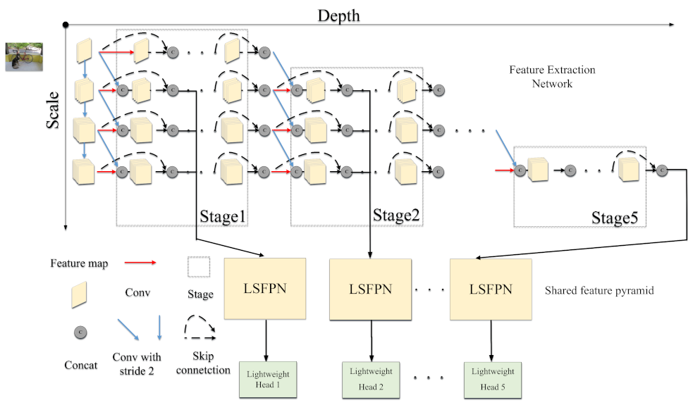
3.2. The Overall Network Architecture

We construct an one-stage detector with feature pyramid structure. Similar to MSDNet, we adopt a multiscale architecture and dense connections. Lightweight shared feature pyramid network and lightweight detection head network are proposed to adapt to the multiscale architecture. The overall network architecture of the dynamic object detection algorithm is shown in Figure 1. The entire network is composed of three parts: a feature extraction network, a shared feature pyramid and a lightweight detection head network. We will introduce the above three parts in detail.

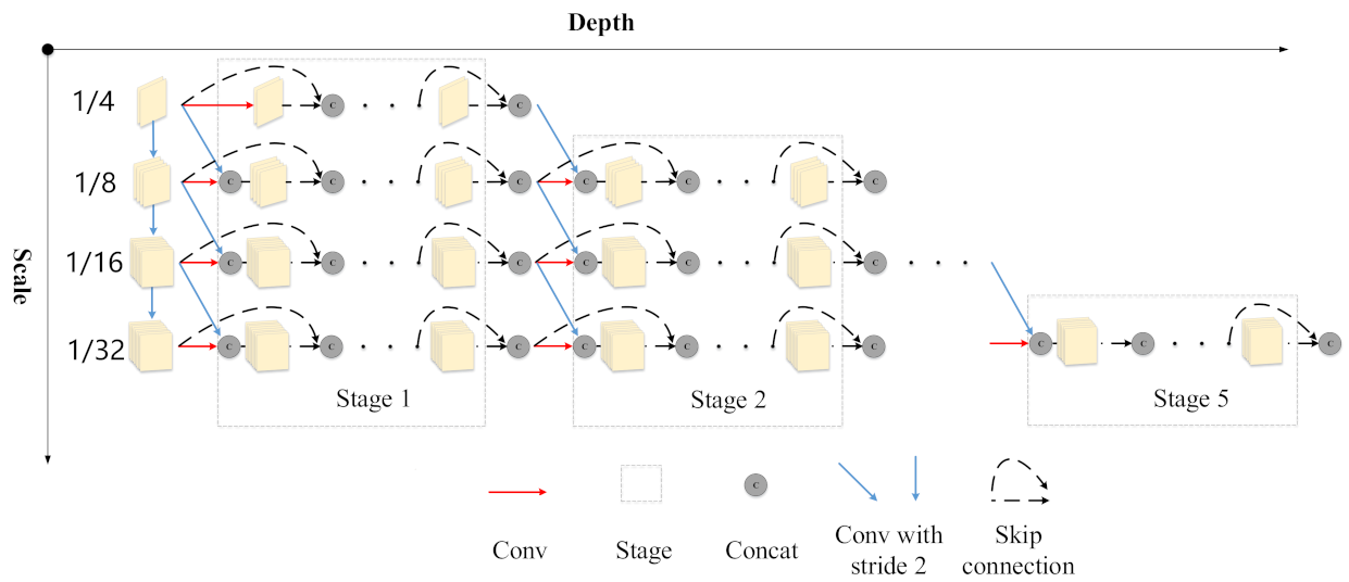
3.2.1. Feature Extraction Network Based on Multiscale Dense Connection

To construct a model that can stop reasoning at any time and return the prediction result, the feature extraction network is critical. When the depth of the current layer is relatively shallow, the feature layer has only low-level high-resolution information, and does not have enough high-level semantic information, which has a great impact on the performance of the shallow detection head. When multiple detection heads are connected behind the feature extraction network, the feature layer tends to optimize the detection heads that close to its depth, which will affect the performance of the latter detection head. To solve these problems, we adopt the feature extraction network based on multiscale dense connections. As shown in Figure 2, we first use a 7 × 7 convolution followed by 2 × 2 average pooling layer to obtain a 1/4 scale (relative to the original input) feature map. To alleviate the problem of insufficient semantic information of shallow layers, multiple conv layers with stride 2 are used to construct feature maps of multiple scales, which are gradually propagated forward in parallel.
On each parallel branch, we use a densely connected network. The resulting features are fused through concatenation with the next layer. Such a shortcut connection can enhance feature reuse, and the features generated in the shallow layer can be directly used by the deeper layer, further suppressing the problem of gradient vanish. At the same time, the dense connection allows the previous features to be directly used by the subsequent network, which reduces the impact of the previous detection heads on the performance of the subsequent heads. When the number of densely connected channels becomes larger and larger, we use a 1 × 1 convolution to reduce the number of channels. In general, we can see that the features of the conv layer of each branch come from the output of the previous layer, the shortcut connection of the previous layer, and the feature map of the previous scale. This is to ensure that the information between branches of different scales can be transmitted.
For a certain conv layer of any branch, its input only comes from the layer in front of the branch and the layer in front of the same position of the previous branch, and has nothing to do with the layers in other positions. Therefore, the forward propagation of the network is a downward ladder. As shown in Figure 2, after a certain number of network layers, the model discards a feature map of a scale until only the feature map with the smallest scale is left. In order to construct a dynamic model, every few layers must take features from the feature extraction network and input them to the corresponding pyramid network. In our setting, we only take the feature maps of the three scales of 1/8, 1/16 and 1/32 (more details can be seen in Section 3.3). The feature maps of these three scales are sent to the corresponding feature pyramid network to obtain five feature maps of different scales: 1/8, 1/16, 1/32, 1/64 and 1/128.

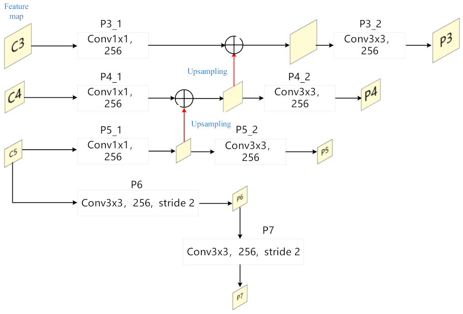
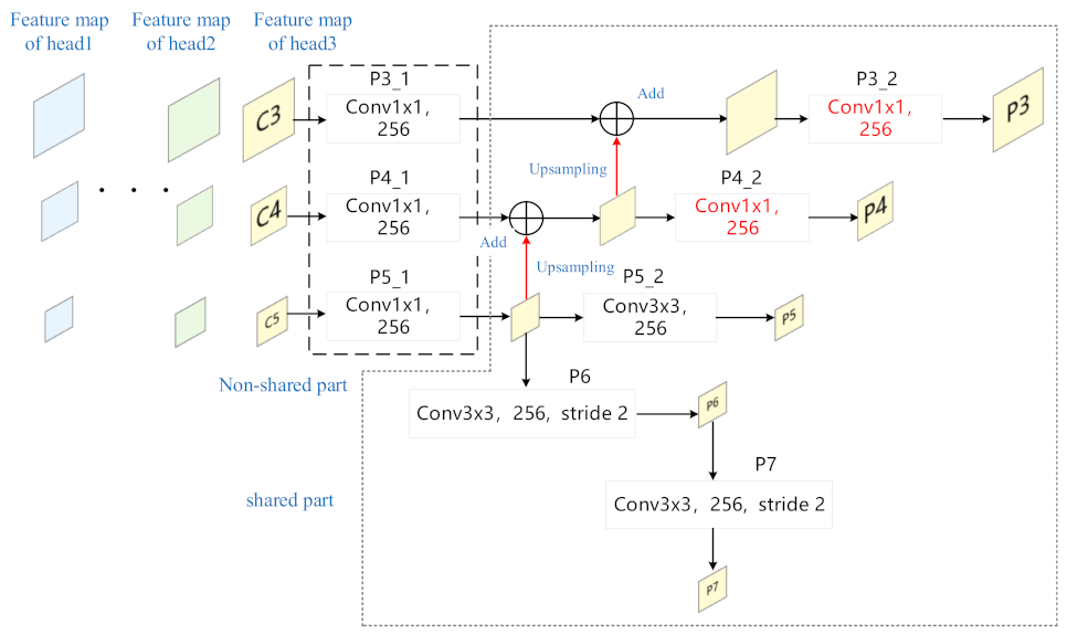
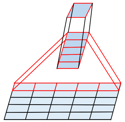
3.2.2. Lightweight Shared Feature Pyramid Network

Nowadays, the Feature pyramid networks (FPN) [38] has become the basic configuration of the object detection model. It can fuse the strong semantics of high-level features and the high resolution of low-level features, bringing significant performance improvements, especially on small objects. However, when the network expands to a dynamic model that can stop inference at any time and return the prediction result, the model has multiple detection heads and the computation and parameter amount of the FPN will have a linear relationship with the number of detection heads. To construct a dynamic object detection model, the computation amount and parameter amount of the feature pyramid brought by multiple detection heads need to be optimized.
Figure 3 shows the structure of FPN. C3, C4 and C5 represent the three-scale feature maps of 1/8, 1/16 and 1/32 introduced in the previous section. They first pass through a 1 × 1 conv layer, corresponding to P3_1, P4_1 and P5_1. The output of the P5_1 layer is upsampled and added with the output of P4_1 layer to obtain a 1/16-scale fused feature map. This feature map is up-sampled and added to the feature map generated by P3_1 to obtain a 1/8-scale fusion Feature map. After a 3 × 3 conv layer, P3_2, P4_2 and P5_2, respectively, we finally obtain the input feature maps P3, P4 and P5. In addition, C5 passes through a 3 × 3 conv layer with a stride 2 to obtain the P6 feature map, and P6 obtains P7 in the same way. Therefore, the input feature maps of the FPN are all generated, P3, P4, P5, P6, P7, and their scales relative to the original image are 1/8, 1/16, 1/32, 1/64, 1/128, respectively.
As RetinaNet is one of the classic object detection models with FPN structure, we take RetinaNet as an example to analyze the distribution of the computation amount (GFlops) and parameter amount (Params) of FPN. As shown in Table 3, the computation and parameter percentages of each conv layer in the feature pyramid are calculated. It can be seen that the main computation amount of the FPN is concentrated on the P3_2 layer and P4_2 layer, which account for 54.6% and 13.7% respectively. This is because they are 3 × 3 conv and their inputs are relatively large-scale feature maps. In the parameter line, we can see that the parameter is mainly concentrated on the P6 layer, since the input channel number of this layer is relatively large. In order to optimize the computation and parameter amount of FPN in the multidetector head model, we propose the lightweight shared feature pyramid network (LSFPN).
As shown in Figure 4, we make three main improvements to FPN: First, to reduce the amount of parameters, we construct a shared feature pyramid network structure, so that all the feature maps required by the detection head share a feature pyramid network. Specifically, the P3_1, P4_1, and P5_1 layer are not shared because the number of feature map channels of different detection head is not consistent. Second, the kernel size of P3_2 and P4_2 layers are changed from 3 × 3 to 1 × 1, which greatly reduces the computation amount of FPN. Third, originally, the P6 layer was directly connected to the feature map C5, and the number of channels of the feature map C5 i = was not fixed, which would cause the P6 layer to be unable to share. In order to optimize the huge amount of parameter of P6 layer, we modify the original structure and connect the P6 layer to the output of P5_ layer. This reduces the parameter amount of P6 layer on the one hand, and on the other hand allows it to be shared. A large number of experiments and analyses verify the effectiveness of the proposed method.

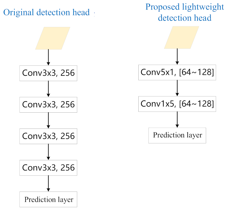
3.2.3. Lightweight Detection Head Network

In constructing a dynamic object detection model, another problem is the amount of computation and parameters number of the detection head network. For both the classification and regression branches, the original RetinaNet stacks four 3 × 3 conv layers followd by a 3 × 3 conv layer as a prediction layer to output the predictions. The entire detection head branch accounts for 52.5% of the total calculation volume and 45.3% of the total parameter volume. In a word, the increase in computation and parameter amount brought by multiple detection heads needs to be optimized.
In order to solve the huge amount of computation and parameters brought by the increase of the detection head network, in this paper, we propose a lightweight detection head network. As shown in Figure 5, we changed the four 3 × 3 conv layers in the original network to a 5 × 1 and 1 × 5 conv layer, and the number of channels has been changed from 256 to between 64 and 128. In this way, the computation amount of the detection head network will be greatly reduced, which is conducive to the expansion of the detection model to multiple detection heads.
The specific process of 5 × 1 convolution and 1 × 5 convolution is shown in Figure 6. A 5 × 1 conv layer is followed by a 1 × 5 conv layer. In this way, the sum of the two is close to the computation amount of a 3 × 3 convolution, but the receptive fields reaches 5 × 5. This alleviates the problem of insufficient receptive fields after reducing the number of conv layers. A large number of experiments and analyses have proved the effectiveness of the proposed algorithm.

3.3. Detailed Structure of the Dynamic Model

In our implementation, the dynamic object detection network proposed in this paper uses a multiscale densely connected feature extraction network. The specific settings when constructing the network are: 5 stages, 4 scales, 7 layers in each stage, a total of 35 layers and 4 branches in parallel. After the first layer, a 1 × 1 conv layer is inserted every 8 layers of the network to reduce the number of channels, so as to prevent the number of channels caused by dense connections from being too large, and the current largest-scale feature layer will be discarded at this time. Since a scale is discarded every certain number of layers, the number of conv layers in each scale is not consistent. In order to uniformly select the feature layers required by each detection head from the feature extraction network, we separately select the feature maps of the three scales of C3, C4 and C5. For the feature map C3, the feature map we choose for it is the 4th, 7th, 10th, 14th and 18th layers on the 1/8 scale; for the feature map C4, the selected features maps are the 5th, 10th, 15th, 21st and 27th layers on the 1/16 scale; for the feature map C5, the selected feature maps are the 7th on the 1/32 scale Layer, 14th layer, 21st layer, 28th layer and 35th layer. Such a one-to-one corresponding combination completes the selection of five detection heads, each with three scale features. The channel numbers of the feature maps of the five detection heads are (192 C 3 , 448 C 4 , 576 C 5 ), (288 C 3 , 768 C 4 , 640 C 5 ), (384 C 3 , 704 C 4 , 608 C 5 ), (320 C 3 , 608 C 4 , 1056 C 5 ), (448 C 3 , 992 C 4 , 976 C 5 ). The subscript indicates the feature map corresponding to the number of channels. The five groups of feature maps are sent to the lightweight shared feature pyramid for feature fusion, and the fused features are sent to the lightweight detection head network for prediction. The lightweight detection head network uses a conv layer with a kernel size of 3 × 3 and a channel number of 64 in the first two heads. The latter three heads use the proposed lightweight detection head, with the number of channels being 96, 96, 128.
In order to conduct comparative experiments on the proposed algorithms, we construct a multiple detector based on MSDNet, ResNet and DenseNet, which are referred to as, respectively, MSDNet_MD, ResNet_MD and DenseNet_MD.
For MSDNet_MD, the structure of the feature extraction network is consistent with ours. After extracting five groups of feature maps from the feature extraction network, they are sent to the five feature pyramid networks for feature fusion, and then sent to the corresponding detection head. Among them, the feature fusion part uses FPN, and the detection head is consistent with RetinaNet, which is formed by stacking 4 3 × 3 convolutions.
For ResNet_MD, the feature extraction network uses ResNet-50. ResNet-50 consists of 3, 4, 6 and 3 residual blocks in conv2-x, conv3-x, conv4-x and conv5-x stages, respectively. In order to uniformly select the feature layer required by each detection head from the feature extraction network, we select the output feature map of conv2-x as the feature map of the first detection head, and the output feature map of conv3-x is the second detection head. The output of the third residual block of conv4-x is the feature map of the third detection head, the output feature map of conv4-x is the input of the fourth detection head, and the output feature map of conv5-x is the input of the fifth detection head. Since the feature map of ResNet is single-scale, some processing is needed. After conv2-x, we connect 3 conv layers, with kernel size 3 × 3, stride 2 and 256 channels, to obtain 1/8, 1/16 and 1/32-scale feature maps. The number of channels are 256, 256, and 256, respectively. In a similar way, we obtain five groups of feature maps of five detection heads. The number of channels are (256 C 3 , 256 C 4 , 256 C 5 ), (512 C 3 , 256 C 4 , 256 C 5 ), (512 C 3 , 1024 C 4 , 256 C 5 ), (512 C 3 , 1024 C 4 , 256 C 5 ), (512 C 3 , 1024 C 4 , 2048 C 5 ). The detection head is consistent with RetinaNet, which is formed by stacking four 3 × 3 convolutions.
For DenseNet_MD, we use DenseNet-201 as the backbone. The output feature of Dense Block1 is selected as the feature map of the first detection head, the output feature of Dense Block2 is the feature map of the second detection head, and the output of the 24th convolution block of Dense Block3 is the input of the third detection head. The output feature map of Dense Block3 is the feature map of the fourth detection head, and the output feature map of Dense Block4 is the output feature map of the fifth detection head.

4. Experimental Results and Discussion

To demonstrate the effectiveness of our approach, we conducted experiments on the PASCAL VOC dataset [52] and RSOD dataset [53]. PASCAL VOC contains 16,551 images and objects from 20 predefined categories annotated with bounding boxes. We use the union of VOC2007 and VOC2012 trainval as training set and evaluate our models on the VOC 2007 test set. RSOD dataset is an open dataset for object detection in remote sensing images. The dataset includes 6950 objects in four categories: aircraft, oil tank, playground and overpass.

4.1. Implementation Details

For fair comparisons, all experiments are implemented based on PyTorch and GeForce RTX 3090 GPU. We use the SGD as the optimizer for model learning. Weight decay of 0.0001 and momentum of 0.9 are used. In order to prevent the initial learning rate from being too large, we use the warmup strategy [4], The learning rate changes as:
lr = lr 1 1 iter num 500 ( 1 0.001 )
lr refers to the learning rate, iter_um is the current number of iterations, 500 refers to the number of iterations set to warmup, and 0.001 refers to the initial learning rate of warmup. After the warmup, the learning rate is set to lr = 0.03 × (batch size)/16, where batch size is set to 8, the number of training epochs is 16, and the learning rate is reduced to 0.3 times the initial learning rate at the 11th epoch. At the 14th epoch, it will be 0.1 times the initial learning rate, and at the 16th epoch, it will be reduced to 0.01 times the initial learning rate. Input images are resized to a maximum scale of 1000 * 600 for PASCAL VOC, without changing the aspect ratio. Horizontal image flipping is the only form of data augmentation.

4.2. Loss Functions

The loss of the k-th detection head is the weighted sum of the classification loss and the regression loss of the positive and negative samples. The specific formula is as follows:
L ( p , t ) k = 1 N i L c l s p k i , p i + λ i p i L r e g t k i , t i
λ is the weight of the regression loss, and N is the number of positive samples. L c l s is the classification loss function, which specifically represents the Focal Loss loss function. L r e g is the regression loss function, which represents the Smooth L1 loss function. The total loss of all detection heads is defined as:
Loss = k w k L ( p , t ) k
where w k is the loss weight of the k-th detection head. In this paper, λ is set to 1, the Focal Loss parameter α is set to 0.25, and γ is set to 2. Anchors are assigned to ground-truth object boxes using an intersection-over-union (IoU) threshold of 0.5, and to background if their IoU is in [0, 0.4). Regarding the setting of the loss weight of the multiple detector head, the weight used for the extraction network with the multiscale densely connected network as the feature is (1, 1, 1, 1, 2). The model using ResNet and DenseNet as the feature extraction network uses (1,1,1,1,1). The reason for this is that the shallow features of ResNet and DenseNet do not have enough semantic information, and the performance of the previous detection heads is relatively poor, so setting their weights to be more average is conducive to the performance improvement of the previous detection heads.

4.3. Analysis of LSFPN

We compare and analyze the origin FPN and the lightweight shared feature pyramid proposed in this paper in terms of calculation amount, parameter amount, and performance. The experimental settings are: the feature extraction network is ResNet-50, and the number of channels of the three layers C3, C4 and C5 sent to the FPN are 512, 1024 and 2048, respectively. From Table 4, it is clear that the LSFPN is on the three convolutional layers of P3_2, P4_2 and P6, and the amount of calculation and parameters are much smaller than that of the FPN. In terms of the amount of accumulated calculations and parameters, the LSFPN is better than the FPN.
As for under the condition of multiple detection heads, the relevant settings of this experiment are the feature extraction network is MSDNet, and the channel numbers of the feature maps of the five heads taken from the feature extraction network are (192 C 3 , 488 C 4 , 576 C 5 ) and 288 C 3 , 768 C 4 , 640 C 5 ), (384 C 3 , 704 C 4 , 608 C 5 ), (320 C 3 , 608 C 4 , 1056 C 5 ), (448 C 3 , 992 C 4 , 976 C 5 ), the detection head network is consistent with the original RetinaNet, the computation amount and parameter amount in the table is the cumulative amount, such as Head = 3 represents the cumulative value of the calculated amount of FPN and the parameter amount of the first three heads. From the experimental results in Table 5, it can be obtained that due to the relatively small amount of calculation of the LSFPN, when the number of detection heads increases, the amount of calculation and parameters does not increase much. This is because most layers of LSFPN share the feature maps of each detection head. On the contrary, when the number of detection heads of FPN increases, the amount of calculations and parameters have also doubled. The number of input feature channels of the three conv layers of P3_1, P4_1 and P5_1 is not fixed, so the size of the convolution cannot be fixed, resulting in the inability to share. When the detection head increases, the increased parameter amount comes from these three convolutional layers. In addition, in terms of performance, it can be found that after the introduction of LSFPN, the performance of the five detection heads is slightly improved, which shows that setting too many FPNs to build a dynamic object detection model will introduce a large number of parameters, which may lead to overfitting. Our LSFPN reduces the amount of parameters, suppresses overfitting and slightly improves performance.

4.4. Analysis of Lightweight Detection Head Network

We compare and analyze the common detection head network and the lightweight detection head network proposed in this paper in terms of calculation amount, parameter amount and performance. The feature extraction network is MSDNet, and the channel numbers of the feature maps of the five heads taken from the feature extraction network are (192, 488, 576), (288, 768, 640), (384, 704, 608), (320, 608, 1056), (448, 992, 976), the feature fusion part uses ordinary FPN, the calculation amount and parameter amount in the table is the cumulative amount, for example, Head = 3 represents the cumulative value of the calculation and parameter values of the first three detection heads.
From Table 6, we can find that regardless of the amount of calculation and parameters or the number of detection heads, the lightweight detection head network (called Light Head here) is nearly 1/10 of the calculation and parameter volume of the ordinary detection head network (called Normal Head here). It shows that the proposed lightweight detection head network effectively reduces the amount of calculation and parameters of the detection head. In addition, it can be found that although the calculation and parameter amount of the lightweight detection head network is much smaller than that of the ordinary detection head network, it can achieve comparable performance, which once again proves the effectiveness of the proposed algorithm.

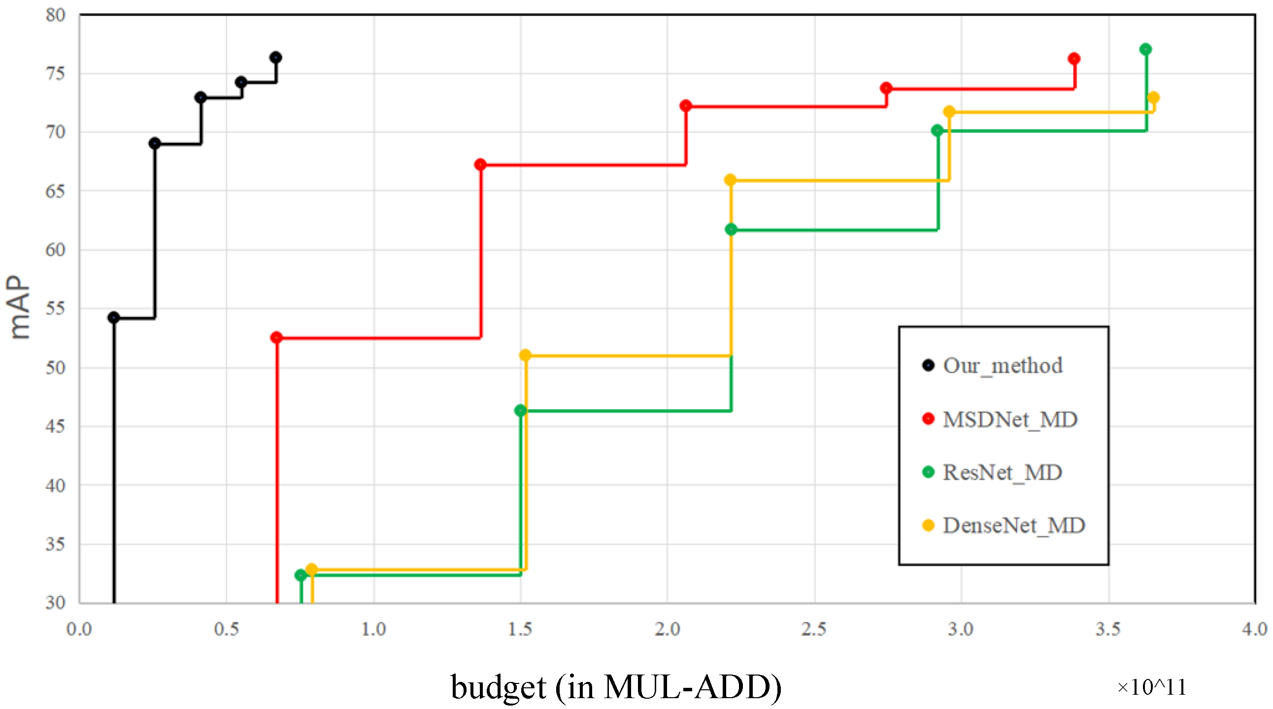
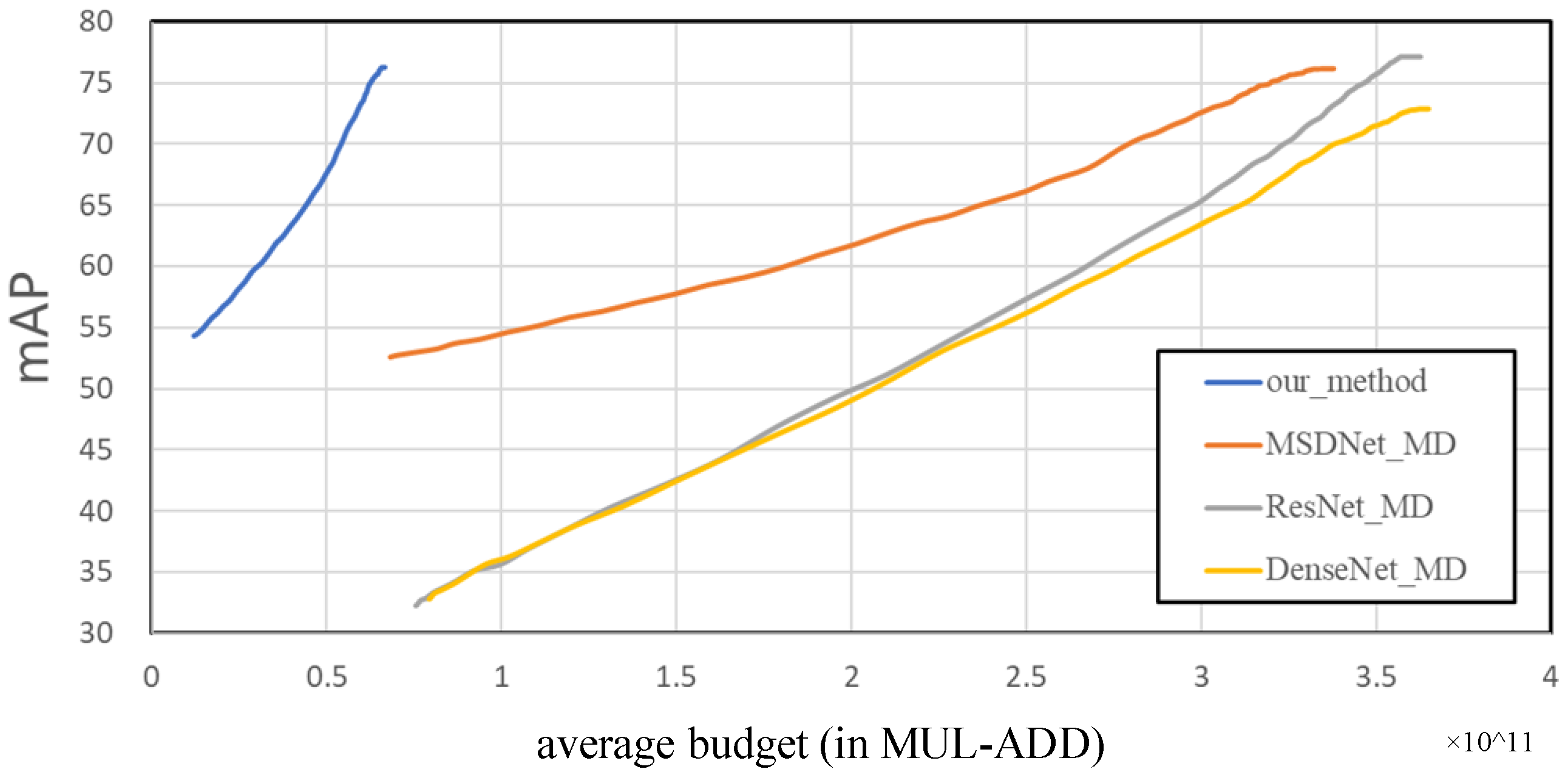
4.5. Experiments Results under Resource-Constrained Conditions

In this section, we report on experiments under resource-constrained conditions are performed on the PASCAL VOC dataset. The specific settings are as proposed in MSDNet, which are mainly experiments under two settings. One is “prediction at any time”, which refers to stopping the prediction at any time and returning the detection result to measure the computational consumption and accuracy at this time. The second is “budgeted batch object detection”, which refers to the use of a fixed calculation budget to reason about the entire test set.
For the “prediction at any time” experiment, we use a feature extraction network based on multiscale dense connections, and the feature fusion part uses the proposed LSFPN, the detection head uses the lightweight detection head network proposed in our paper. Comparison methods include MSDNet_MD, ResNet_MD, DenseNet_MD, which are multihead detectors constructed with MSDNet, ResNet and DenseNet, respectively. It can be seen from Figure 7 that the performance of the detection heads in front of ResNet_MD and DenseNet_MD is significantly lower than that of MSDNet_MD and our method. The main reason is that the shallow features of ResNet and DenseNet do not have sufficient high-level semantic information. The calculation amount of our entire network is lower than that of the first detection heads of MSDNet_MD, ResNet_MD and DenseNet_MD, which once again proves the superiority of the proposed LSFPN and lightweight detection head network. Under the same mAP, the calculation amount of the proposed algorithm is about 1/5 of that of models such as MSDNet_MD, ResNet_MD and DenseNet_MD.
For the “budgeted batch object detection” experiment, we used the entire PASCAL VOC2007 test set, with a total of 4952 images, and the average calculation amount of these 4952 images is used as the calculation budget. The experimental results are shown in Figure 8. It can be seen that MSDNet_MD uses a multiscale dense connection network for its feature extraction network, so its performance is much better than that of ResNet_MD and DenseNet_MD when the preliminary calculation budget is low. Their performance is relatively close when the computational budget is large. This shows that the feature extraction network based on multiscale dense connection is beneficial to construct feature maps of various scales in the shallow layer, which is beneficial to improve the performance of the previous detection head. The method proposed in our paper, when the calculation budget is close to MSDNet_MD, ResNet_MD and DenseNet_MD, our performance is much better than them. When the performance is close to them, the calculation budget is only less than 1/5 of them.

4.6. Evaluation on RSOD Dataset

We evaluate our model on the RSOD dataset [53], which is a large remote sensing object detection dataset with four categories: aircraft, oiltank, playground and overpass. The format of this dataset is PASCAL VOC. The entire dataset was divided into a training data set and a validation data set at a ratio of 5:1. The results in Table 7 show consistent performance with PASCAL VOC. The proposed method achieves better performance with a smaller calculation amount.

4.7. Discussions

To further investigate the advantage of the proposed method in this study, we conducted the ablation experiment of the proposed algorithm. The head network used in the experiment is the original RetinaNet detection head, which is called Normal Head (NH) here, and the lightweight detection head network proposed in our paper is called Light Head (LH). It can be seen from Table 8 that, compared to the Normal Head, based on the original FPN, the performance of all the five heads of our proposed lightweight detection head is better. Combined with Normal Head, the LSFPN has higher performance of each detection head than the FPN. This fully demonstrates that the network structure proposed in this paper achieves better performance under the condition of lower calculation amount and parameter amount, and verifies the effectiveness of the proposed algorithm. Finally, the LSFPN and the lightweight head network are combined to achieve good performance.
We further conducted an experiment on the weight of the loss of multiple detection heads. It can be seen from Table 9 that when the loss weights of each head are averaged, the performance of the front detection head is higher, especially the first and second detection heads, and the latter detection heads, such as the fourth and fifth detection heads. The accuracy is slightly lower. When the weight is (1, 1, 1, 1, 2), the accuracy of the last detection head is significantly improved, and the performance of the first two heads features a certain decline. Considering that the dynamic object detection model uses a densely connected feature extraction network, it has an advantage over other models in the performance of the previous detection head, so the final use of our paper is the weight (1, 1, 1, 1, 1, 2), so that both the front and back detection heads can show the superiority.
The qualitative results are provided in Figure 9. As shown in Figure 9, the first column to the fifth column are the detection results of the detection head 1 to the detection head 5. It can be seen from the figure that the detection head 1, having fewer feature extraction network layers and limited depth, is prone to false detection due to the insufficient semantic information. The detection heads at the back of the network have relatively few false detections. For some relatively simple samples, the detection result of the second detection head is actually acceptable, and there is no need for forward propagation to the fifth detection head. We can see that our method has consistent performance in different scenarios (such as sky, outdoor and indoor), which shows the robustness of our method. This once again illustrates the effectiveness and significance of the proposed algorithm. It is worth mentioning that our dynamic detector can be deployed easily without any heuristic processing and special operations. The whole model would be loaded first and ”easy” samples would be output at shallow exits without executing deeper layers to accelerate the speed. During deployment, as our model is defined in PyTorch, we first convert it into the ONNX format and then run it with ONNX Runtime, which is a performance-focused engine that can inferences efficiently across multiple platforms and hardware.

5. Conclusions

This paper proposes a dynamic object detection algorithm that can stop predicting and returning the detection result at any time. In order to achieve dynamic prediction, this paper constructs a detection network with multiple detection heads. Specifically, in order to improve the performance of the shallow detection head, a multiscale densely connected feature extraction network is used as the backbone of the detection model. In order to reduce the huge amount of calculation and parameters brought by the feature pyramid in the dynamic model, this paper proposes a lightweight shared feature pyramid network, which greatly reduces the increase in the calculation and parameter amount of the FPN when designing a detection model with multiple detection heads. In order to reduce the huge amount of calculation and parameters brought by the multiple detection head when constructing the dynamic object detection model, we propose a lightweight detection head network, which reduces the calculation amount of the detection head while maintaining the original performance. Finally, a large number of experiments verify the effectiveness of our method.

Author Contributions

L.Z. and Z.X. have equal contribution to this work and are co-first authors. Conceptualization, L.Z. and Z.X.; methodology, L.Z. and Z.X.; software, Z.X. and J.L.; validation, Z.X., J.L. and Y.Q.; writing—original draft preparation, L.Z. and Z.X.; writing—review and editing, L.Z. and L.L.; supervision, W.T.; project administration, L.L.; funding acquisition, L.L. and W.T. All authors have read and agreed to the published version of the manuscript.

Funding

This work was supported in part by the National Natural Science Foundation of China (Grant 61976227, 62176096 and 61991412).

Institutional Review Board Statement

Not applicable.

Informed Consent Statement

Not applicable.

Data Availability Statement

The data presented in this study are available on request from the first author.

Acknowledgments

The authors are grateful to the Editor and reviewers for their constructive comments, which significantly improved this work.

Conflicts of Interest

The authors declare no conflict of interest.

References

  1. Krizhevsky, A.; Sutskever, I.; Hinton, G.E. Imagenet classification with deep convolutional neural networks. Adv. Neural Inf. Process. Syst. 2012, 25, 1097–1105. [Google Scholar] [CrossRef]
  2. Simonyan, K.; Zisserman, A. Very deep convolutional networks for large-scale image recognition. arXiv 2014, arXiv:1409.1556. [Google Scholar]
  3. Szegedy, C.; Liu, W.; Jia, Y.; Sermanet, P.; Reed, S.; Anguelov, D.; Erhan, D.; Vanhoucke, V.; Rabinovich, A. Going deeper with convolutions. In Proceedings of the IEEE Conference on Computer Vision and Pattern Recognition, Boston, MA, USA, 7–12 June 2015; pp. 1–9. [Google Scholar]
  4. He, K.; Zhang, X.; Ren, S.; Sun, J. Deep residual learning for image recognition. In Proceedings of the IEEE Conference on Computer Vision and Pattern Recognition, Las Vegas, NV, USA, 27–30 June 2016; pp. 770–778. [Google Scholar]
  5. Howard, A.G.; Zhu, M.; Chen, B.; Kalenichenko, D.; Wang, W.; Weyand, T.; Andreetto, M.; Adam, H. Mobilenets: Efficient convolutional neural networks for mobile vision applications. arXiv 2017, arXiv:1704.04861. [Google Scholar]
  6. Hu, J.; Shen, L.; Sun, G. Squeeze-and-excitation networks. In Proceedings of the IEEE Conference on Computer Vision and Pattern Recognition, Salt Lake City, UT, USA, 18–23 June 2018; pp. 7132–7141. [Google Scholar]
  7. Han, K.; Wang, Y.; Tian, Q.; Guo, J.; Xu, C.; Xu, C. Ghostnet: More features from cheap operations. In Proceedings of the IEEE/CVF Conference on Computer Vision and Pattern Recognition, Seattle, WA, USA, 13–19 June 2020; pp. 1580–1589. [Google Scholar]
  8. Hubara, I.; Courbariaux, M.; Soudry, D.; El-Yaniv, R.; Bengio, Y. Binarized neural networks. Adv. Neural Inf. Process. Syst. 2016, 29. [Google Scholar]
  9. Jacob, B.; Kligys, S.; Chen, B.; Zhu, M.; Tang, M.; Howard, A.; Adam, H.; Kalenichenko, D. Quantization and training of neural networks for efficient integer-arithmetic-only inference. In Proceedings of the IEEE Conference on Computer Vision and Pattern Recognition, Salt Lake City, UT, USA, 18–23 June 2018; pp. 2704–2713. [Google Scholar]
  10. Zhuang, Z.; Tan, M.; Zhuang, B.; Liu, J.; Guo, Y.; Wu, Q.; Huang, J.; Zhu, J. Discrimination-aware channel pruning for deep neural networks. arXiv 2018, arXiv:1810.11809. [Google Scholar]
  11. Singh, P.; Verma, V.K.; Rai, P.; Namboodiri, V.P. Play and prune: Adaptive filter pruning for deep model compression. arXiv 2019, arXiv:1905.04446. [Google Scholar]
  12. Xiao, X.; Wang, Z. Autoprune: Automatic network pruning by regularizing auxiliary parameters. Adv. Neural Inf. Process. Syst. 2019, 32. [Google Scholar]
  13. Huang, G.; Chen, D.; Li, T.; Wu, F.; van der Maaten, L.; Weinberger, K.Q. Multi-scale dense networks for resource efficient image classification. arXiv 2017, arXiv:1703.09844. [Google Scholar]
  14. Yang, L.; Han, Y.; Chen, X.; Song, S.; Dai, J.; Huang, G. Resolution adaptive networks for efficient inference. In Proceedings of the IEEE/CVF Conference on Computer Vision and Pattern Recognition, Seattle, WA, USA, 13–19 June 2020; pp. 2369–2378. [Google Scholar]
  15. Bolukbasi, T.; Wang, J.; Dekel, O.; Saligrama, V. Adaptive neural networks for efficient inference. In Proceedings of the International Conference on Machine Learning, PMLR, Sydney, Australia, 6–11 August 2017; pp. 527–536. [Google Scholar]
  16. Ruiz, A.; Verbeek, J. Adaptative inference cost with convolutional neural mixture models. In Proceedings of the IEEE/CVF International Conference on Computer Vision, Seoul, Korea, 27 October–2 November 2019; pp. 1872–1881. [Google Scholar]
  17. Wang, X.; Yu, F.; Dou, Z.Y.; Darrell, T.; Gonzalez, J.E. Skipnet: Learning dynamic routing in convolutional networks. In Proceedings of the European Conference on Computer Vision (ECCV), Munich, Germany, 8–14 September 2018; pp. 409–424. [Google Scholar]
  18. Lin, T.Y.; Goyal, P.; Girshick, R.; He, K.; Dollár, P. Focal loss for dense object detection. In Proceedings of the IEEE International Conference on Computer Vision, Venice, Italy, 22–29 October 2017; pp. 2980–2988. [Google Scholar]
  19. Girshick, R.; Donahue, J.; Darrell, T.; Malik, J. Rich feature hierarchies for accurate object detection and semantic segmentation. In Proceedings of the IEEE Conference on Computer Vision and Pattern Recognition, Columbus, OH, USA, 23–28 June 2014; pp. 580–587. [Google Scholar]
  20. Uijlings, J.R.; Van De Sande, K.E.; Gevers, T.; Smeulders, A.W. Selective search for object recognition. Int. J. Comput. Vis. 2013, 104, 154–171. [Google Scholar] [CrossRef] [Green Version]
  21. Zitnick, C.L.; Dollár, P. Edge boxes: Locating object proposals from edges. In Proceedings of the European Conference on Computer Vision, Zurich, Switzerland, 6–12 September 2014; pp. 391–405. [Google Scholar]
  22. Girshick, R. Fast r-cnn. In Proceedings of the IEEE International Conference on Computer Vision, Santiago, Chile, 7–13 December 2015; pp. 1440–1448. [Google Scholar]
  23. Ren, S.; He, K.; Girshick, R.; Sun, J. Faster r-cnn: Towards real-time object detection with region proposal networks. Adv. Neural Inf. Process. Syst. 2015, 28, 91–99. [Google Scholar] [CrossRef] [PubMed] [Green Version]
  24. Dai, J.; Li, Y.; He, K.; Sun, J. R-fcn: Object detection via region-based fully convolutional networks. Adv. Neural Inf. Process. Syst. 2016, 379–387. [Google Scholar]
  25. Cai, Z.; Vasconcelos, N. Cascade r-cnn: Delving into high quality object detection. In Proceedings of the IEEE Conference on Computer Vision and Pattern Recognition, Salt Lake City, UT, USA, 18–23 June 2018; pp. 6154–6162. [Google Scholar]
  26. Redmon, J.; Divvala, S.; Girshick, R.; Farhadi, A. You only look once: Unified, real-time object detection. In Proceedings of the IEEE Conference on Computer Vision and Pattern Recognition, Las Vegas, NV, USA, 27–30 June 2016; pp. 779–788. [Google Scholar]
  27. Redmon, J.; Farhadi, A. YOLO9000: Better, faster, stronger. In Proceedings of the IEEE Conference on Computer Vision and Pattern Recognition, Honolulu, HI, USA, 21–26 July 2017; pp. 7263–7271. [Google Scholar]
  28. Liu, W.; Anguelov, D.; Erhan, D.; Szegedy, C.; Reed, S.; Fu, C.Y.; Berg, A.C. Ssd: Single shot multibox detector. In Proceedings of the European Conference on Computer Vision, Amsterdam, The Netherlands, 8–16 October 2016; pp. 21–37. [Google Scholar]
  29. Huang, R.; Pedoeem, J.; Chen, C. YOLO-LITE: A real-time object detection algorithm optimized for non-GPU computers. In Proceedings of the 2018 IEEE International Conference on Big Data (Big Data), Seattle, WA, USA, 10–13 December 2018; pp. 2503–2510. [Google Scholar]
  30. Uddin, M.S.; Hoque, R.; Islam, K.A.; Kwan, C.; Gribben, D.; Li, J. Converting Optical Videos to Infrared Videos Using Attention GAN and Its Impact on Target Detection and Classification Performance. Remote Sens. 2021, 13, 3257. [Google Scholar] [CrossRef]
  31. Zhu, J.Y.; Park, T.; Isola, P.; Efros, A.A. Unpaired image-to-image translation using cycle-consistent adversarial networks. In Proceedings of the IEEE International Conference on Computer Vision, Venice, Italy, 22–29 October 2017; pp. 2223–2232. [Google Scholar]
  32. Tian, Z.; Shen, C.; Chen, H.; He, T. FCOS: Fully Convolutional One-Stage Object Detection. arXiv 2019, arXiv:1904.01355. [Google Scholar]
  33. Zhu, C.; He, Y.; Savvides, M. Feature selective anchor-free module for single-shot object detection. In Proceedings of the IEEE Conference on Computer Vision and Pattern Recognition, Seoul, Korea, 27 October–2 November 2019; pp. 840–849. [Google Scholar]
  34. Law, H.; Deng, J. Cornernet: Detecting objects as paired keypoints. In Proceedings of the European Conference on Computer Vision (ECCV), Munich, Germany, 8–14 September 2018; pp. 734–750. [Google Scholar]
  35. Duan, K.; Bai, S.; Xie, L.; Qi, H.; Huang, Q.; Tian, Q. Centernet: Keypoint triplets for object detection. In Proceedings of the IEEE International Conference on Computer Vision, Seoul, Korea, 27 October–2 November 2019; pp. 6569–6578. [Google Scholar]
  36. Tan, M.; Pang, R.; Le, Q.V. Efficientdet: Scalable and efficient object detection. In Proceedings of the IEEE/CVF Conference on Computer Vision and Pattern Recognition, Seattle, WA, USA, 13–19 June 2020; pp. 10781–10790. [Google Scholar]
  37. Radosavovic, I.; Kosaraju, R.P.; Girshick, R.; He, K.; Dollár, P. Designing network design spaces. In Proceedings of the IEEE/CVF Conference on Computer Vision and Pattern Recognition, Seattle, WA, USA, 13–19 June 2020; pp. 10428–10436. [Google Scholar]
  38. Lin, T.Y.; Dollár, P.; Girshick, R.; He, K.; Hariharan, B.; Belongie, S. Feature pyramid networks for object detection. In Proceedings of the IEEE Conference on Computer Vision and Pattern Recognition, Honolulu, HI, USA, 21–26 July 2017; pp. 2117–2125. [Google Scholar]
  39. Liu, S.; Qi, L.; Qin, H.; Shi, J.; Jia, J. Path aggregation network for instance segmentation. In Proceedings of the IEEE Conference on Computer Vision and Pattern Recognition, Salt Lake City, UT, USA, 18–23 June 2018; pp. 8759–8768. [Google Scholar]
  40. Wang, J.; Chen, K.; Xu, R.; Liu, Z.; Loy, C.C.; Lin, D. Carafe: Content-aware reassembly of features. In Proceedings of the IEEE/CVF International Conference on Computer Vision, Seoul, Korea, 27 October–2 November 2019; pp. 3007–3016. [Google Scholar]
  41. Ghiasi, G.; Lin, T.Y.; Le, Q.V. Nas-fpn: Learning scalable feature pyramid architecture for object detection. In Proceedings of the IEEE/CVF Conference on Computer Vision and Pattern Recognition, Seoul, Korea, 27 October–2 November 2019; pp. 7036–7045. [Google Scholar]
  42. Zhu, M.; Han, K.; Yu, C.; Wang, Y. Dynamic Feature Pyramid Networks for Object Detection. arXiv 2020, arXiv:2012.00779. [Google Scholar]
  43. Veit, A.; Belongie, S. Convolutional networks with adaptive inference graphs. In Proceedings of the European Conference on Computer Vision (ECCV), Munich, Germany, 8–14 September 2018; pp. 3–18. [Google Scholar]
  44. Wu, Z.; Nagarajan, T.; Kumar, A.; Rennie, S.; Davis, L.S.; Grauman, K.; Feris, R. Blockdrop: Dynamic inference paths in residual networks. In Proceedings of the IEEE Conference on Computer Vision and Pattern Recognition, Salt Lake City, UT, USA, 18–23 June 2018; pp. 8817–8826. [Google Scholar]
  45. Lin, J.; Rao, Y.; Lu, J.; Zhou, J. Runtime neural pruning. In Proceedings of the 31st International Conference on Neural Information Processing Systems, Long Beach, CA, USA, 4–9 December 2017; pp. 2178–2188. [Google Scholar]
  46. Hu, H.; Dey, D.; Hebert, M.; Bagnell, J.A. Learning anytime predictions in neural networks via adaptive loss balancing. In Proceedings of the AAAI Conference on Artificial Intelligence, Honolulu, HI, USA, 27 January–1 February 2019; Volume 33, pp. 3812–3821. [Google Scholar]
  47. Li, H.; Zhang, H.; Qi, X.; Yang, R.; Huang, G. Improved techniques for training adaptive deep networks. In Proceedings of the IEEE/CVF International Conference on Computer Vision, Seoul, Korea, 27 October–2 November 2019; pp. 1891–1900. [Google Scholar]
  48. Feng, J.; Hua, J.; Lai, B.; Huang, J.; Li, X.; Hua, X.S. Learning to Generate Content-Aware Dynamic Detectors. arXiv 2020, arXiv:2012.04265. [Google Scholar]
  49. Zhou, B.; Khosla, A.; Lapedriza, A.; Oliva, A.; Torralba, A. Learning deep features for discriminative localization. In Proceedings of the IEEE Conference on Computer Vision and Pattern Recognition, Las Vegas, NV, USA, 27–30 June 2016; pp. 2921–2929. [Google Scholar]
  50. Verelst, T.; Tuytelaars, T. Dynamic convolutions: Exploiting spatial sparsity for faster inference. In Proceedings of the IEEE/CVF Conference on Computer Vision and Pattern Recognition, Seattle, WA, USA, 13–19 June 2020; pp. 2320–2329. [Google Scholar]
  51. Xie, Z.; Zhang, Z.; Zhu, X.; Huang, G.; Lin, S. Spatially adaptive inference with stochastic feature sampling and interpolation. In Proceedings of the European Conference on Computer Vision, Online, 23–28 August 2020; pp. 531–548. [Google Scholar]
  52. Everingham, M.; Van Gool, L.; Williams, C.K.; Winn, J.; Zisserman, A. The pascal visual object classes (voc) challenge. Int. J. Comput. Vis. 2010, 88, 303–338. [Google Scholar] [CrossRef] [Green Version]
  53. Long, Y.; Gong, Y.; Xiao, Z.; Liu, Q. Accurate object localization in remote sensing images based on convolutional neural networks. IEEE Trans. Geosci. Remote Sens. 2017, 55, 2486–2498. [Google Scholar] [CrossRef]
Figure 1. The overall network architecture diagram of the dynamic object detection algorithm.
Remotesensing 13 04610 g001
Figure 2. Feature extraction network based on multiscale dense connection.
Remotesensing 13 04610 g002
Figure 3. The structure of FPN given in [38].
Remotesensing 13 04610 g003
Figure 4. The structure of proposed lightweight shared feature pyramid network.
Remotesensing 13 04610 g004
Figure 5. Improvement of our lightweight detection head.
Remotesensing 13 04610 g005
Figure 6. A 5 × 1 conv layer is followed by a 1 × 5 conv layer.
Remotesensing 13 04610 g006
Figure 7. Performance of anytime prediction models as a function of computational budget on the Pascal voc. Higher is better.
Remotesensing 13 04610 g007
Figure 8. Performance of budgeted batch object detection models as a function of average computational budget per image the on Pascal voc. Higher is better.
Remotesensing 13 04610 g008
Figure 9. Qualitative comparison between different detection head on Pascal voc dataset. The first column to the fifth column are the detection results of the detection head 1 to the detection head 5.
Remotesensing 13 04610 g009
Table 1. Analysis of MSDNet’s computation and parameter amount.
MSDNetHead1Head2Head3Head4Head5
GFlops5.6G13G20.9G27.3G28.4G
Params2.2M5.6M9.9M14.5M16.8M
Table 2. Analysis of RetinaNet’s computation and parameter amount.
RetinaNetBackboneFPNHeadAccumulated Amount
GFlops40.8G8.5G54.5G103.8G
GFlops(%)39.38.252.5-
Params23.518M26.09M57.6G
Params(%)40.813.945.3-
Table 3. The distribution of the computation amount (GFlops) and parameter amount (Params) of FPN.
FPNP3_1P3_2P4_1P4_2P5_1P5_2P6P7
GFlops(%)12.154.66.113.733.46.80.2
Params(%)1.67.43.37.46.57.4597.4
Table 4. Analysis of LSFPN’s computation and parameter amount under a single detection head.
LayersFPN (GFlops)LSFPN (GFlops)FPN (Params)LSFPN (Params)
P3_11.02G1.02G0.13M0.13M
P3_24.60G0.51G0.59M0.066M
P4_10.51G0.51G0.26M0.26M
P4_21.15G0.13G0.59M0.066M
P5_10.37G0.37G0.52M0.52M
P5_20.29G0.29G0.59M0.59M
P6_10.065G0.008G4.7M0.59M
P7_20.002G0.002G0.59M0.59M
Accumulated8G2.84G8M2.81M
Table 5. Analysis of LSFPN’s computation and parameter amount under multiple detection heads.
Nums of HeadHead = 1Head = 2Head = 3Head = 4Head = 5
FPN (GFlops)6.95G14.28G21.75G29.25G37.16G
LSFPN (GFlops)1.72G3.81G6.05G8.17G10.73G
FPN (Params)4M8.6M12.8M18.1M23.3M
LSFPN (Params)2.22M2.66M3.1M3.61M4.23M
FPN (mAP)52.567.272.273.776.2
LSFPN (mAP)53.467.872.573.976.4
Table 6. Analysis of Light Head’s computation and parameter amount under multiple detection heads.
Nums of HeadHead = 1Head = 2Head = 3Head = 4Head = 5
Normal Head (GFlops)54.54G109.1G163.6G218.2G272.7G
Light Head (GFlops)4.38G8.76G14.25G19.73G27.48G
Normal Head (Params)26.1M52.2M78.3M104.4M130.5M
Light Head (Params)2.1M4.2M6.82M9.44M13.15M
Normal Head (mAP)52.567.272.273.776.2
Light Head (mAP)54.769.072.674.076.3
Table 7. Performance of anytime prediction models on the RSOD dataset.
MethodHead = 1Head = 2Head = 3Head = 4Head = 5
MSDNet_MD (GFlops)69.61G140.52G220.73G276.85G339.12G
MSDNet_MD (mAP)81.9888.8089.0789.2889.39
ResNet_MD (GFlops)76.91G151.42221.35G280.03G362.18G
ResNet_MD (mAP)60.1275.4986.2889.0389.41
DenseNet_MD (GFlops)80.62G156.72G221.49G292.38G365.21G
DenseNet_MD (mAP)61.5672.3486.3287.1589.27
Our (GFlops)14.05G30.87G49.65G66.22G80.37G
Our (mAP)82.1488.8589.1289.3189.40
Table 8. Ablation experiment of LSFPN and LH.
Method/mAPHead = 1Head = 2Head = 3Head = 4Head = 5
FPN+NH52.567.272.273.776.2
FPN+LH54.76972.67476.3
LSFPN+NH53.467.872.573.976.4
LSFPN+LH54.269.072.974.276.3
Table 9. Ablation experiments of the loss weight of different detection head.
Loss Weight/mAPHead = 1Head = 2Head = 3Head = 4Head = 5
1 , 1 , 1 , 1 , 1 55.569.973.174.174.6
1 , 1 , 1 , 1 , 2 54.269.072.974.276.3
Publisher’s Note: MDPI stays neutral with regard to jurisdictional claims in published maps and institutional affiliations.

