Technical Note

Partial Shape Recognition for Sea Ice Motion Retrieval in the Marginal Ice Zone from Sentinel-1 and Sentinel-2

Earth Observation and Modelling, Department of Geography, Kiel University, Ludewig-Meyn-Str. 14, 24098 Kiel, Germany
*
Author to whom correspondence should be addressed.
Remote Sens. 2021, 13(21), 4473; https://doi.org/10.3390/rs13214473
Submission received: 14 September 2021 / Revised: 3 November 2021 / Accepted: 4 November 2021 / Published: 8 November 2021
(This article belongs to the Special Issue Remote Sensing Monitoring of Arctic Environments)

Abstract

:
We present an algorithm for computing ice drift in the marginal ice zone (MIZ), based on partial shape recognition. With the high spatial resolution of Sentinel-1 and Sentinel-2 images, and the low sensitivity to atmospheric influences of Sentinel-1, a considerable quantity of ice floes is identified using a mathematical morphology method. Hausdorff distance is used to measure the similarity of segmented ice floes. It is tolerant to perturbations and deficiencies of floe shapes, which enhances the density of retrieved sea ice motion vectors. The PHD algorithm can be applied to sequential images from different sensors, and was tested on two combined image mosaics consisting of Sentinel-1 and Sentinel-2 data acquired over the Fram Strait; the PHD algorithm successfully produced pairs of matched ice floes. The matching result has been verified using shape and surface texture similarity of the ice floes. Moreover, the present method can naturally be extended to the problem of multi-source sea ice image registration.

1. Introduction

The importance of sea ice motion mainly arises from its impact on climate studies. Information on sea ice motion is required by studies including (1) regional exchange of sea ice, e.g., sea ice drifting towards lower latitudes, where it finally melts, (2) the formation of leads and ridges by ice divergence and shear, (3) air-sea ice-ocean interaction (energy fluxes) as regional ice motion imposes a velocity boundary condition on the ocean surface [1], and (4) the formation and maintenance of polynyas [2]. In the context of the shrinking Arctic Sea ice and the expansion of open water, marine transport and offshore activities in the Arctic are expected to increase steadily, especially in the marginal ice zone (MIZ) [3]. In the MIZ, drifting ice plays an important role in protecting the stable morphology of the inner ice from wave penetration [4], and impacts human accessibility to the Arctic Ocean [5]. Therefore, monitoring of sea ice features such as ice islands and multi-year (MY) ice becomes necessary to prevent hazards [6].
In the literature, different approaches to retrieve sea ice motion from various sources of satellite remote sensing data can be found. Most of these algorithms derive the drift of patterns or features in two sequential sea ice images by means of pattern matching (PM), feature tracking (FT), or the optical flow approach [7]. Maximum-cross-correlation (MCC) and normalized cross-correlation (NCC) have been applied in PM algorithms [8,9]. Another method used in PM algorithms is phase-correlation (PC) [10]. Compared to MCC and NCC methods, PC can capture rotated features [11]. FT algorithms such as scale invariant feature transform (SIFT) [12] and speed-up robust feature (SURF) [13] identify key points in the image, and then track the motion of these key points. The oriented FAST and rotated BRIEF (ORB) algorithm is proposed to improve the computationally efficient and robust features to image noise of FT algorithms [14].
Most of the aforementioned algorithms are performed for continuous ice cover [8,14] or piecewise continuous ice cover [7,9]. Sea ice motion in summer MIZ of low sea ice concentration (SIC), however, remains largely unstudied. MCC and NCC are based on the similarity of sub-domains in the images. As opposed to closed sea ice, sub-domain images in the MIZ are characterized by the presence of a constantly moving collection of discrete floes and open water. When larger leads (open water) exist between the ice floes, they rotate and transit with almost no interaction between each other, which reduces the similarity between the sub-domains in sequenced images, and therefore the floes show only a weak correlation (the lower the sea ice concentration, the more difficult for MCC and NCC methods). Compared to patterns or specific image features, the shape of floes is more invariant between sequenced images in the MIZ. Therefore, the invariance properties of floe shapes in multisource satellite data (e.g., SAR and optical sensor) become more distinct. We therefore propose this method for sea ice motion retrieval, especially in the MIZ, where existing methods perform less well.
There are two shape-based ice drift algorithms in the literature. One uses a suite of geometrical ice floe parameters (perimeter, major and minor axes, centroid position, and surface and convex area) to identify and track ice floes [15], and another uses the Euclidean distance of the ice floe centroid to the nearest boundary pixel in n directions as a descriptor for floe matching [16]. However, the shape of the same ice floe in two sequenced images may be altered by melting, breaking off, or joining/rafting with surrounding floes, in which case the sea ice motion retrieval requires recognition of partial shape similarity. The Hausdorff distance used in this study has the advantage that it can naturally be extended to the problem of finding the best partial shape similarity between two point sets.
Today, an enormous amount of Earth observation data is freely available for mapping Arctic Sea ice in the MIZ, including active and passive high spatial resolution satellite missions, such as Sentinel-1 (S-1) and Sentinel-2 (S-2). Sea ice drifting, however, hampers the registration of images from different sensors, and impedes long-term monitoring of individual floes. Thus, to overcome this limitation of sea ice monitoring, fine (pixel-to-pixel) sea ice motion information is required. In this paper, we propose an algorithm (PHD) with two main objectives: (1) mapping the drift of discrete floes in the MIZ based on partial shape matching, and (2) pixel-to-pixel registration of ice floes in S-1 and S-2 images.

2. Data

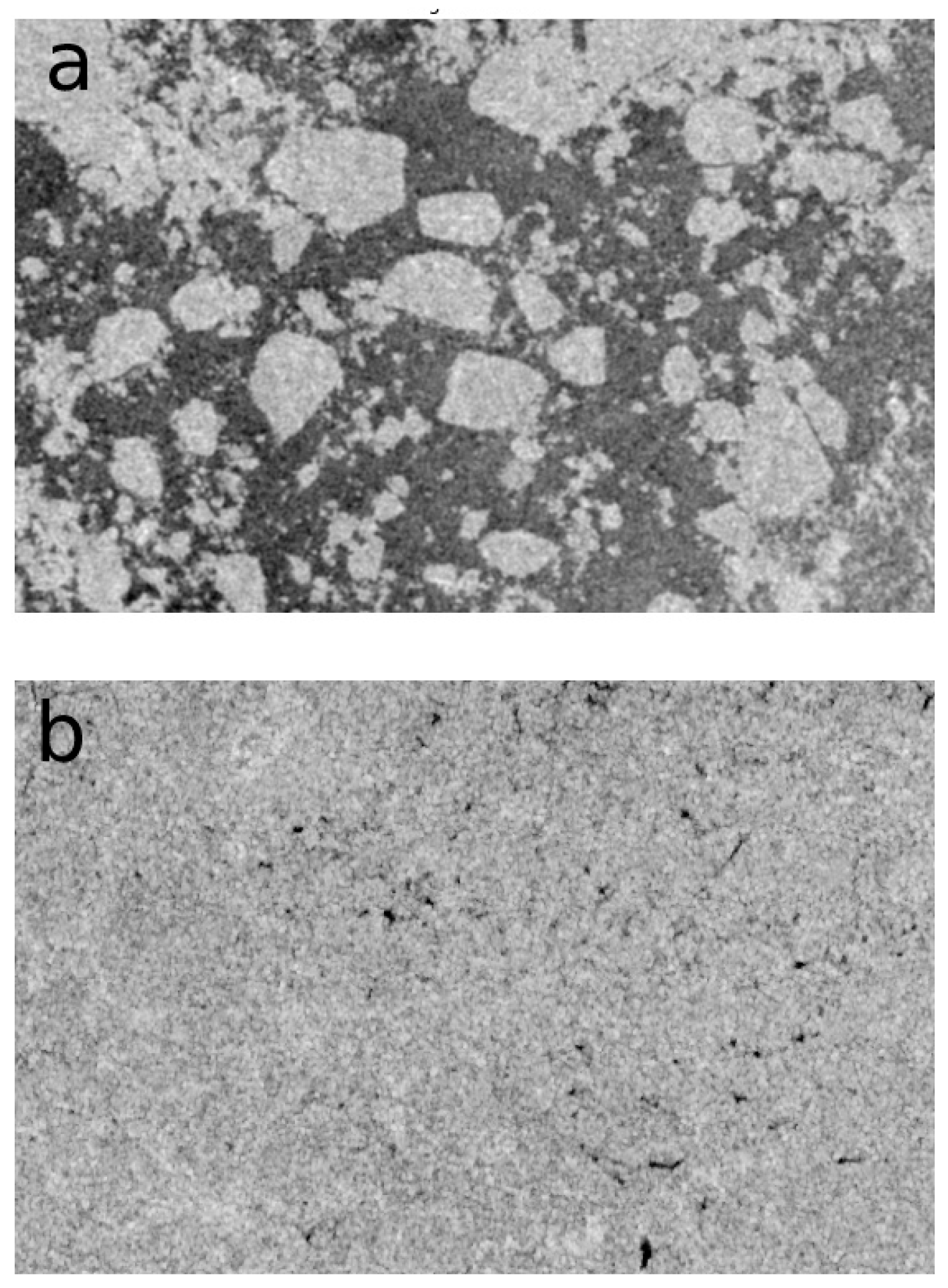
2.1. Sentinel-1 Data

S-1 synthetic aperture radar (SAR) data acquired in extra wide swath mode with medium resolution were used in this study, a stitched mosaic of 16 S-1 tiles of 30 July 2019 is presented in Figure 1. The S-1 mission consists of two satellites, with S-1A and -B launched in April 2014 and 2016, respectively. These two satellites improve temporal resolution, and a large archive already exists. Each tile covers approximately 400 km × 400 km, with a pixel size of 40 m. The large spatial coverage and high spatial resolution of S-1 enables detailed observations of sea ice floes, which, in turn, may be a plus for feature matching. We processed the data on Google Earth Engine (GEE), which provides Level-1 Ground Range Detected (GRD) products. Orbit file application, noise removal, radiometric calibration, and terrain correction were applied. The final pixels contain values of normalized radar cross-section (radar backscatter intensity, denoted as σ 0 ) in HH and HV polarization. For further analysis, we used HH polarization, due to high contrast between ice and open water in HH images [17].

2.2. Sentinel-2 Data

S-2 L2A data were also used in this study, encompassing atmospheric-corrected surface reflectance. Stitched mosaics of 198 S-2 tiles of 30 July 2019 are shown in Figure 1. S-2 is a polar-orbiting, optical mission for land- and coastal region-monitoring and emergency services. The mission is a constellation of two satellites, S-2A and S-2B, each one equipped with an optical imaging sensor MSI (Multi-Spectral Instrument). S-2A and -B were launched in 2015 and 2017, respectively. MSI provides 13 spectral bands between 443 and 2202 nm, and spatial resolutions between 10 and 60 m. S-2 provides high spatial resolution optical images of Arctic Ocean offshore areas up to once a day [18,19,20,21]. We used Band 3 (560 nm), due to the high contrast between ice and open water in this wavelength region [16]; clouds were masked using the ‘QA60’ band.

3. Methodology

The methodological approach follows three consecutive steps of image segmentation, ice floe extraction, and ice floe matching, which are described in the following sections.

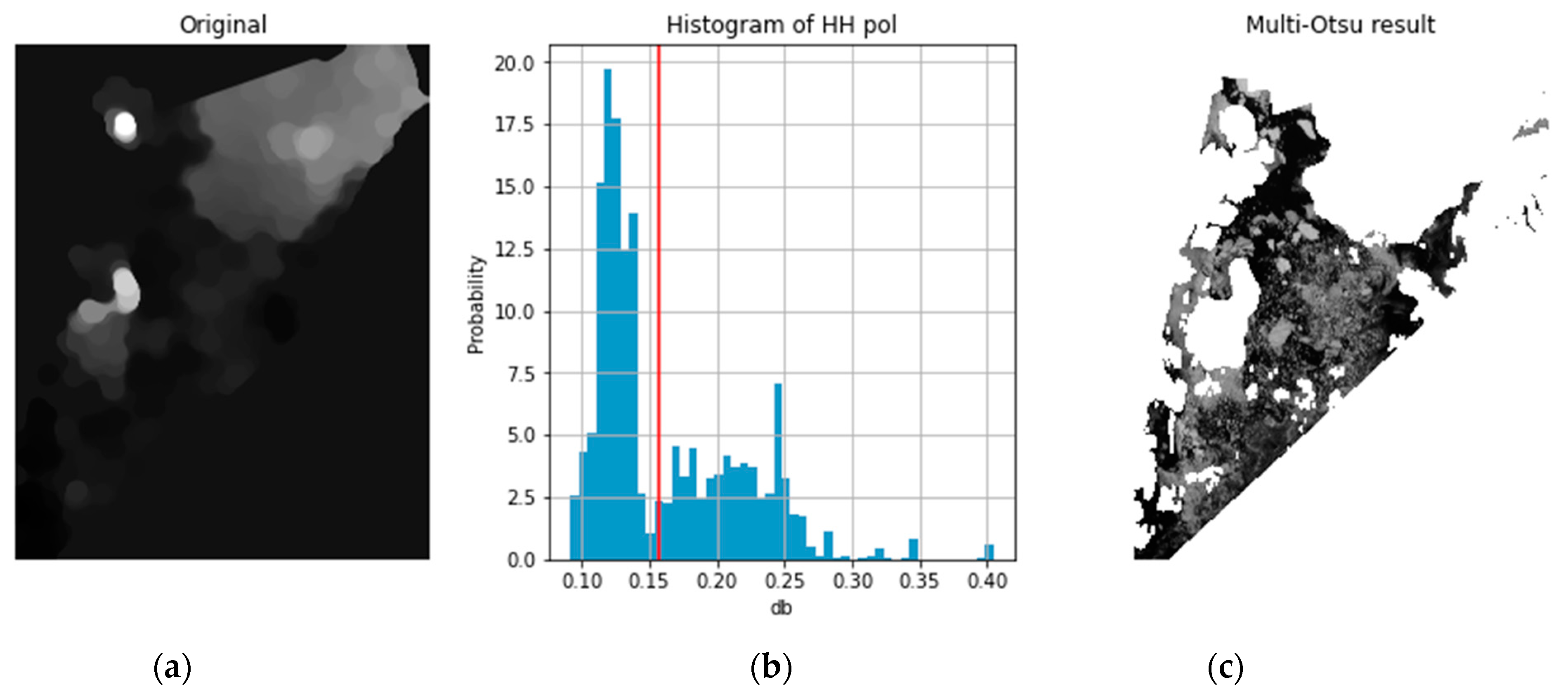
3.1. Image Segementation

To segment MIZ from landfast ice (LFI) and densely packed ice in S1 and S2 data, we utilized mathematical morphology, a theory based on the analysis of spatial patterns, which concerns the characterization of how a structuring element (SE) fits into an image [22]. Inner ice cover, LFI, and sea ice in the MIZ show distinct textures in satellite imagery (Figure 2). The loose MIZ is characterized by a collection of bright discrete particles/floes on a dark background, and the consolidated inner ice cover and LFI have a continuous or piecewise continuous bright texture (Figure 2). To delete LFI and densely packed ice, a morphological opening followed by a morphology closing are applied to the image, with a SE of larger size than that of the ice floes of MIZ:
A = ( ( ( A B ) B ) B ) B
where A is the backscatter (S-1) or surface reflectance (S-2) image, B is a disk-shaped structuring element of 400 × 400 pixels, and and is erosion and dilation operation, respectively. The morphological opening of an image is defined as an erosion followed by a dilation; the morphological closing of an image is defined as a dilation followed by an erosion. Opening can remove small bright spots and connect dark features; this tends to remove discrete ice floes, and close up open water of MIZ. Morphology closing can remove small dark cracks and connect bright features; this tends to remove lead and close up ice cover of inner ice/LFI. The output result A is shown in Figure 3. Due to its low mean density in A , MIZ can be identified using multi-Otsu segmentation; a threshold with a value of 0.16 was used, and sections with a value larger than the threshold were deleted from further processing [23].

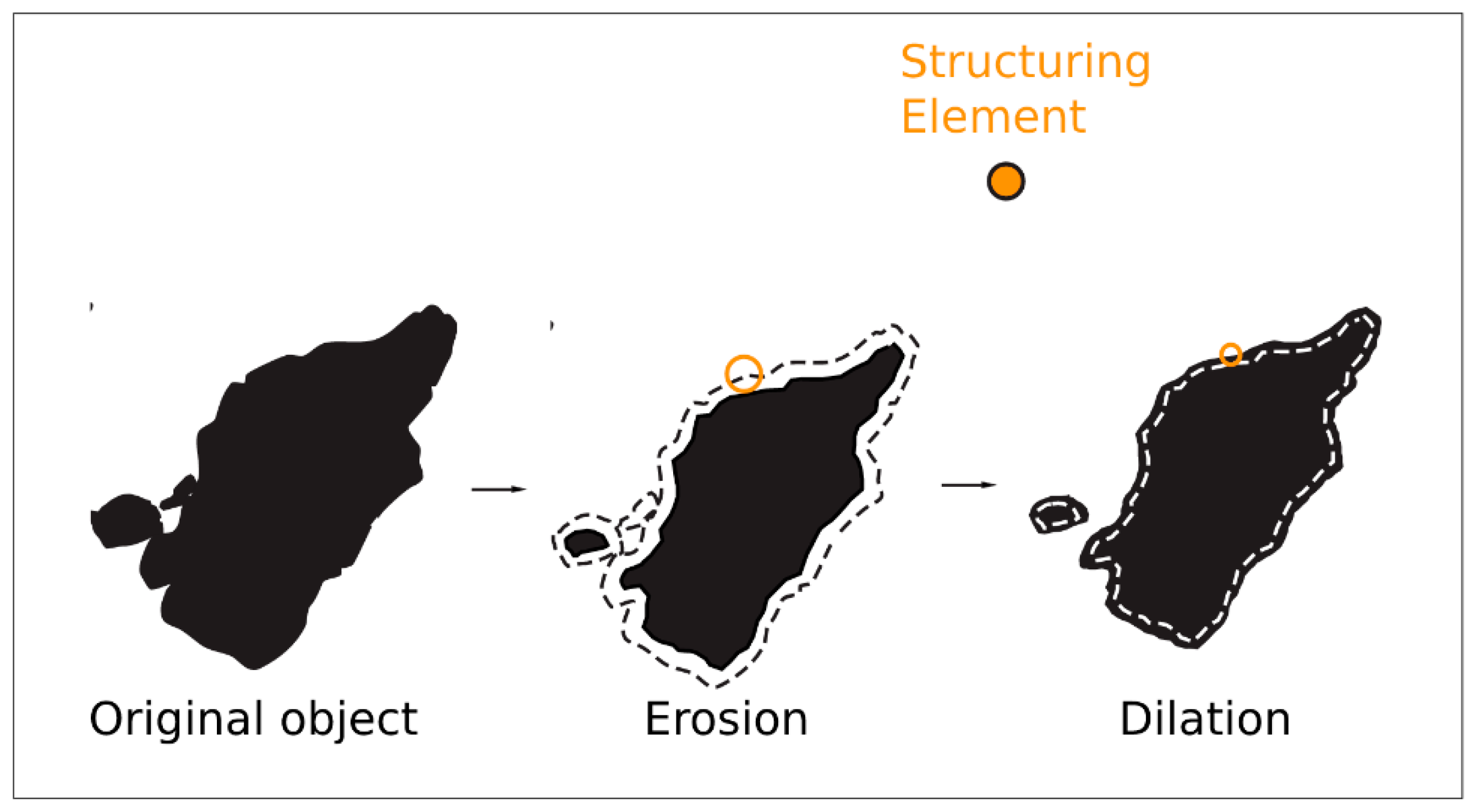
3.2. Ice Floe Extraction

To extract ice floes, the watershed transform method was utilized [24]. A subset of the original image is shown in Figure 4a. First, an elevation map of the image was found using the Sobel gradient (Figure 4c) [25], then markers of the water background and the floes were identified (Figure 4d), based on the extreme values of the grayscale histogram of the subset of image (Figure 4b). Finally, we used the watershed transform to fill regions of the elevation map, starting with the markers determined above. Based on the watershed segmentation result (Figure 4e), we then disconnected ice floes and removed small size brash ice by utilizing a morphology dilation, followed by a morphology erosion (Figure 5). Furthermore, zigzag shaped objects, collections of brash ice, or multiple connected ice floes were removed by thresholding of roundness:
R = 4 × π × S / P 2
where S and P are the area and the perimeter of the object, respectively. Since ice floes tend to have higher roundness, objects of roundness less than 0.7 were removed (Figure 4f). Small ice floes (less than 10,000 pixels) were also removed, due to their limited information of floe edges. In the next section, we provide further details of the algorithm for matching objects using the partial shape similarity concept; in particular, connected ice floes can also be matched.

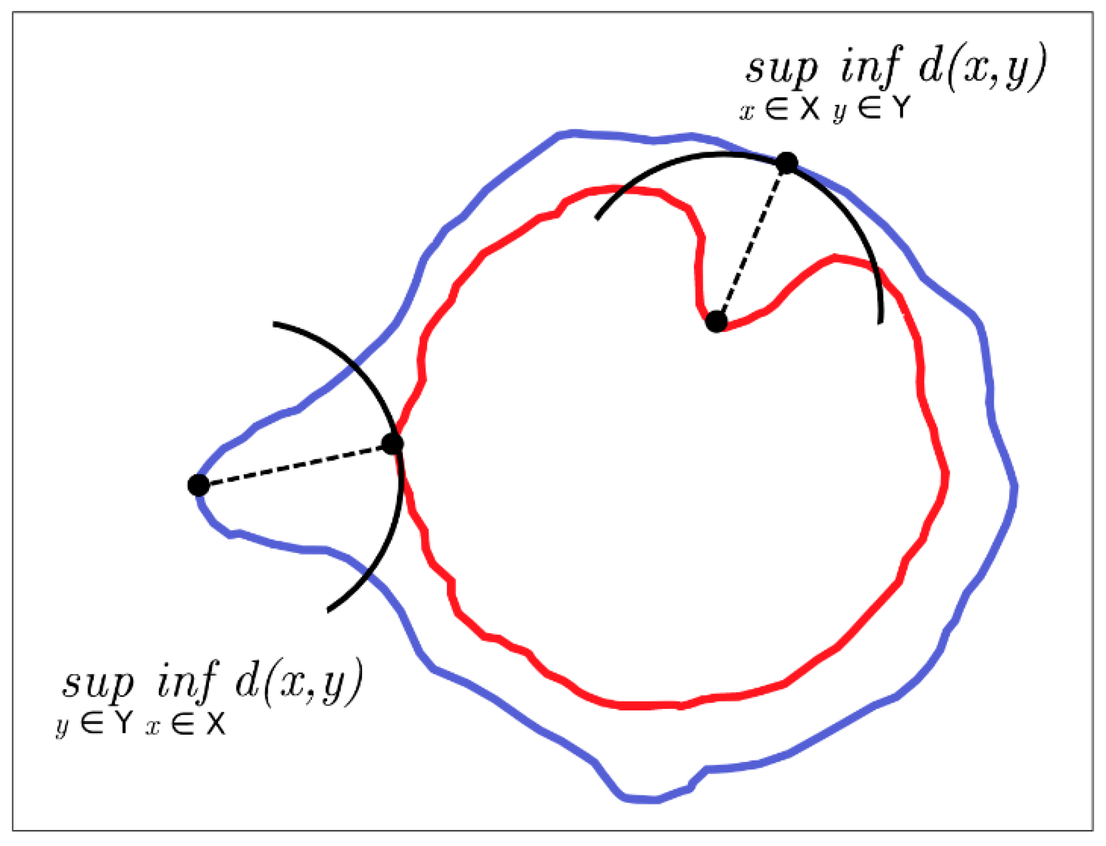
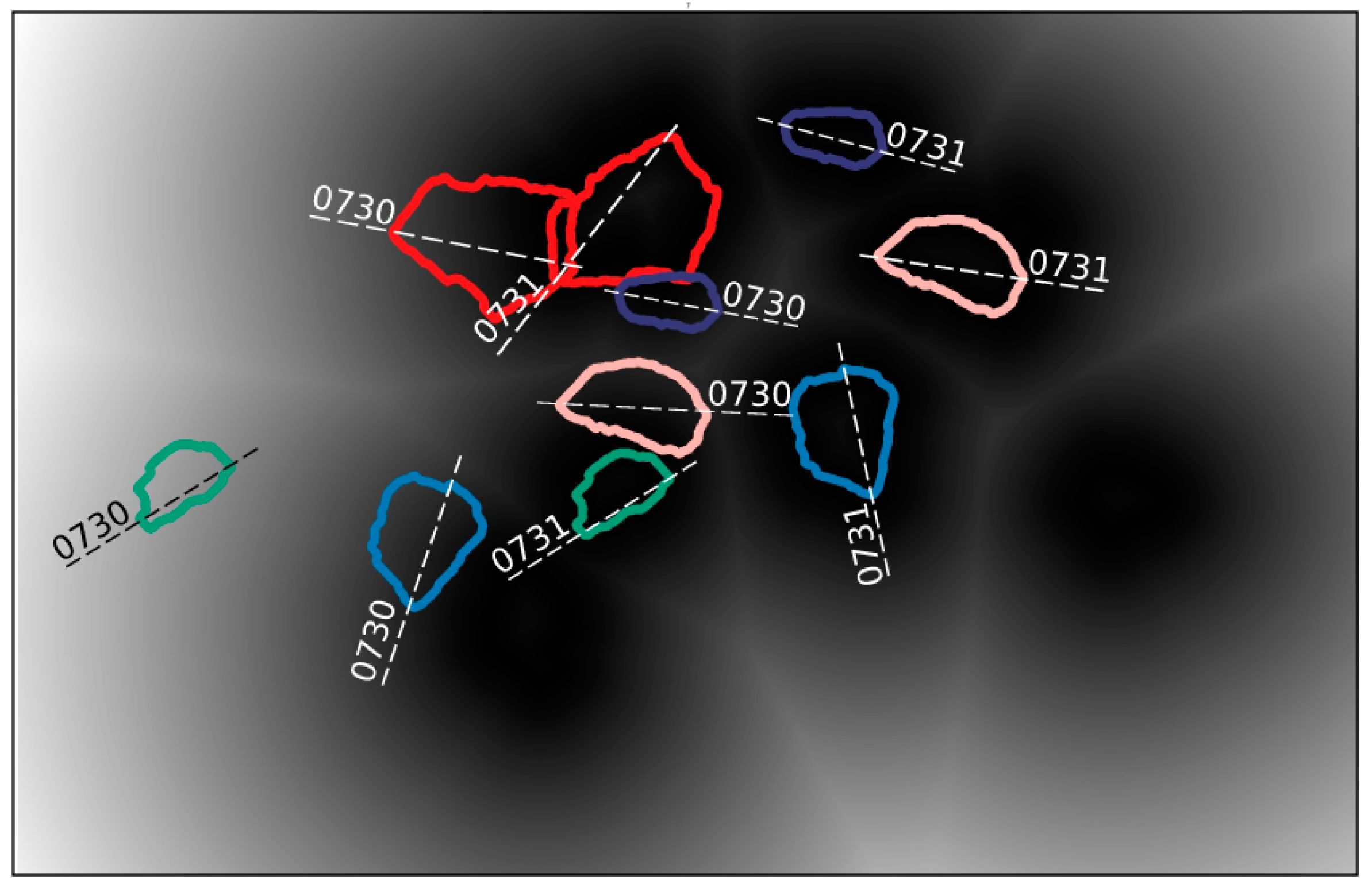
3.3. Ice Floe Matching

As a third step, we applied the Hausdorff Distance for matching the extracted ice floes (Figure 6). The Hausdorff distance measures the extent to which each point of a set lies near some point of another set, and vice versa [26]. Thus, this distance can be used to determine the degree of resemblance between two ice floes or objects. Given two finite point sets X = { x 1 , ,   x p } and Y = { y 1 , ,   y p } , the Hausdorff distance is defined as:
H ( X , Y ) = max ( h ( X , Y ) , h ( Y , X ) )
where:
h ( X , Y ) = sup x X   inf y Y x y
· is some underlying norm on the points of X and Y , sup represents the supremum, and inf represents the infimum. h ( X , Y ) identifies the point x X that is farthest from any point of Y , and measures the distance from x to its nearest neighbor in Y (Figure 6). For computing the Hausdorff distance under rigid motion of ice floe (translation and rotation), we used the Euclidean norm (L2). We fixed the set X , and allowed set Y to move. The minimum value of the Hausdorff distance under rigid (Euclidean) motion M E ( X , Y ) then gives the best transformation of Y with respect to X :
M E ( X , Y ) = min t , θ H ( X , ( R θ Y ) t )
where H is the Hausdorff distance as defined in Equation (3), is the standard Minkowski sum notation, ( R θ Y ) t = { R θ y + t | b Y } , and R θ is the standard rotation matrix. The distance is small when there is a Euclidean transform that brings every point of Y near some point of X , and vice versa.
As mentioned above, the shape of the same ice floe in two sequenced images may be altered by melting, breaking off, or joining/rafting with surrounding floes, in which case the sea ice motion retrieval requires a recognition of partial shape similarity. The Hausdorff distance has the advantage that it can naturally be extended to the problem of finding the best partial shape similarity between two point sets. For simplicity, the computation of h ( X , Y ) determines the distance of the point of set Y that is farthest from any point of X , that is, each point of Y is ranked by the distance to the nearest point of X , and the largest ranked point determine the distance. A natural definition of the distance for K of the q model points ( 1 K q ) is given by taking the K th ranked point of X (rather than the largest ranked one):
h K ( X , Y ) = K b B t h min a A a b
where K b B t h denotes the K th ranked value in the set of distance. This definition of the distance has the advantage that it automatically selects the K best matching points of ice floe X , because it identifies the subset of ice floe X of size K that minimizes the directed Hausdorff distance. In general, some fraction 0 f 1 of the points of floe X must be considered to compute h K ( X , Y ) .
Practically, a Voronoi surface d ( x ) of a set Y was defined for the calculation of h K ( X , Y ) . For each location x , it provides the distance from x to the nearest point y Y . Figure 7 illustrates the Voronoi surface of floes Y (31 July 2019) of a S-1 subset, where brighter (whiter) parts of the image correspond to higher Hausdorff distance values. We can use the Voronoi surface to determine the place where the floes X (30 July 2019) might be in Y (31 July 2019), i.e., we located each floe of 30 July 2019 to the Voronoi surface of the floes in the 31 July dataset under rigid motion (which gave the lowest Hausdorff distance).
Since the approach introduced above requires significant computation time when applied to a large dataset, we applied some techniques for more efficient computation. Firstly, based on the ice floe extraction result, each floe was labelled with the UTM (Universal Transverse Mercator) coordinate ( X , Y ) of its center. For the matching process, we considered only floe pairs with a Euclidean distance of less than 10 km. Additionally, a threshold τ of the Hausdorff distance could be set, and we could stop computing once the Hausdorff distance of current translation was below τ (e.g., 5% of floe size). Secondly, we assumed that floes tend to keep a similar area in sequential images, without strong formation of leads or ridges. Once a floe and its neighboring floes had been extracted in sequential images, we arranged a priority calculation according to the area similarity of each floe pair. Moreover, the computing stopped partway if the floe pairs showed a Hausdorff distance below τ .

4. Experimental Results and Discussion

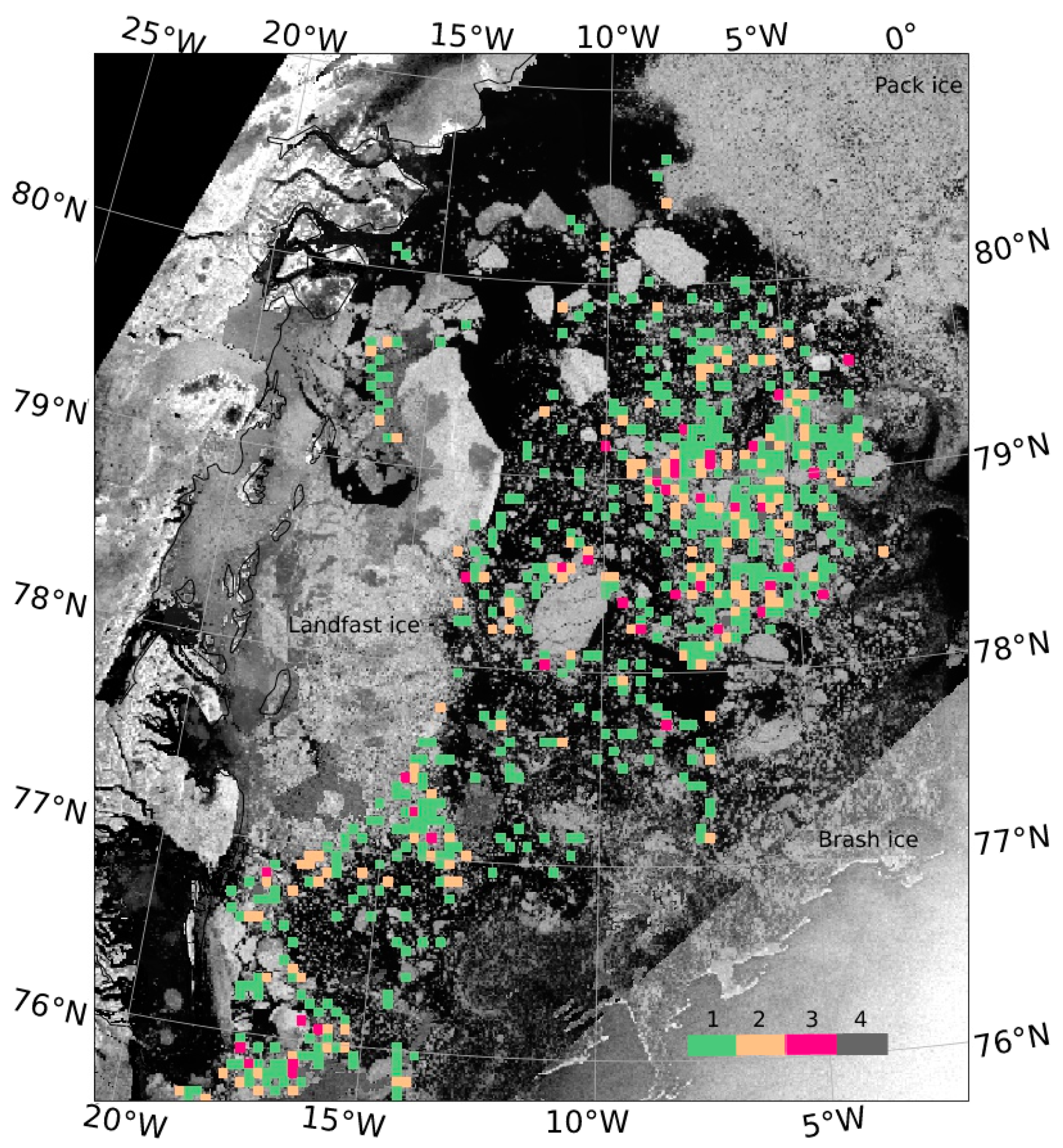
4.1. Ice Floes Drift of MIZ

Sequential S-1 and S-2 images acquired on 30 July 2019 and 31 July 2019 (16 Sentinel-1 and 198 Sentinel-2 images, respectively) over the Fram Strait were processed to estimate the motion of MIZ ice floes. The algorithm identified 8228 ice floes (4394 of 30 July, and 3834 of 31 July), and produced 1388 pairs of matched ice floes (position and number of matched ice floes are shown in Figure 8), i.e., 34% of the extracted ice floes are matched (with the parameter setting presented in the first row in Table 1). Most of the floes were extracted from the S-2 images. When clouds were present in the S-2 images, we filled the clouded areas with pixels of S-1 images.
To validate the results, we manually checked 100 of the matched floes pairs (randomly selected by numbers from 1-1388). The manual check was necessary due to the lack of valid reference data. Ice buoy data may work, but it is rare, and would only be available for one or two floe pairs. The criterion for the manual validation check was that the matched floe pairs must have similar shapes, areas, and surface textures in the satellite images. Table 1 shows the accuracy and computing speed for these floes with different parameter settings.
Using a sufficiently fine-scaled parameter setting, the algorithm retrieves accuracies near 100%. Table 1 indicates that the values of θ / θ and l / l significantly affect the computing time. With increasing step size of translation and rotation from 1/20 to 1/12, the computing time near-linearly decreases from 1849 s to 1289 s, but leads to 2% of mismatched floes. The parameter f also shows a higher effect on accuracy than computing time; its sensitivity may also be related to SIC, because with higher SIC more leads and ridges may be present on the floes. The parameter f also shows a high effect on the value of N , which defines the number of matched floes pairs. As the f-value decreases, pairs of floes with a smaller proportion of similar edges can also be matched, but there will also be some non-matching floes. The parameter τ has a significant effect on both computing time and accuracy and, therefore, can be a key parameter for algorithm tuning. Optimum values of these parameter are achieved when the accuracy requirements are met within the shortest time possible.
To derive the ice floes drift in the MIZ, we calculated a drift vector from each pair of matching ice floes. For this, the starting and end position of the vector are the centroids of the floe in the two sequential images. To illustrate the ice floe motion on a large scale, inverse distance weighting (IDW) was used to retrieve the ice displacement vectors on a 204 × 164 polar stereographic grid (Figure 9). It can be observed from Figure 8 and Figure 9 that the above-mentioned processing may include interpolation inside the MIZ, and extrapolation at the edge of MIZ.
The retrieved sea ice motion indicated that, as opposed to the relatively smooth sea ice motion field of closed ice cover, the motion in MIZ may show sharp and locally extreme spatial gradients. Moreover, the study illustrated some interesting kinematic processes of MIZ sea ice, such as shear flow parallel to the ice edge, interaction between MIZ ice motion, and external conditions in the air and sea; these processes, however, are still largely unstudied.
As mentioned in Section 3.2, we removed small sized brash ice by applying morphology processing. Brash ice is an accumulation of floating ice made up of fragments with diameters less than 2 m. It is usually present at the edge of the MIZ, and connected to open water. The proposed method cannot be applied to brash ice area as the resolution of S-1 and S-2 is too coarse for monitoring the heavily fragmented brash ice. In S-1 and S-2 images, brash ice has a structure like algal spirals. Therefore, an algal spiral tracking algorithm (e.g., by Kozlov et al., 2020 [27]) can be used to retrieve brash ice motion. Combining the proposed method and Kozlov’s algal spiral tracking algorithm may allow for the retrieval of the complete MIZ ice motion field.

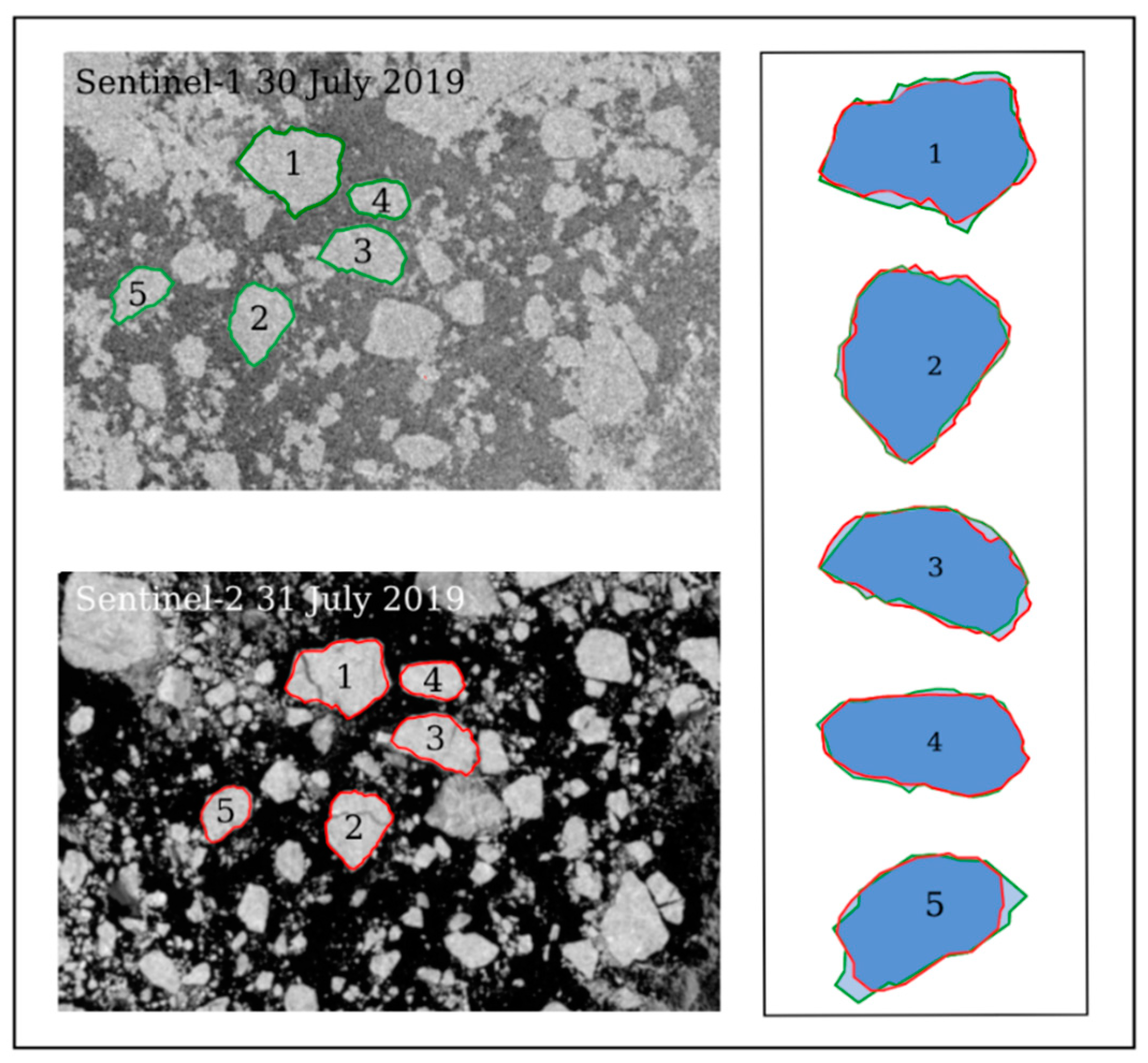
4.2. Ice Floes Imagery Registration

The Hausdorff distance approach can naturally be extended to the problem of co-registration of multi-source sea ice imagery. For sea ice motion retrieval, the co-registration process needs pixel-to-pixel information about the motion (displacement and rotation) of the ice floes. For image co-registration, we utilized the approach of Section 3 to retrieve the matching floe pairs and their rough, relative displacement and rotation (as we utilized coarse computing step size and τ   values to stop the computation partway, the retrieved relative motion shows a coarse precision). Then, we used a smaller calculation step size (1 pixel for location and 1° for rotation) to retrieve the rigid motion that generates the minimum Hausdorff distance. After the floe pairs were matched as precisely as possible, the ice floe images were sub-setted via their overlapping part (Figure 10). As shown in Figure 10, ice floe images from S-1 and S-2 can be merged for further analysis. Using this information, floes can be compared, and information about area change (e.g., due to melting or break off), their rotation and motion speed can be extracted. When applied to sequenced S-2 images, changes in surface albedo or melt pond evolution can be investigated

5. Conclusions

In this paper we developed a sea ice motion tracking algorithm with two objectives: (1) mapping the discrete floes drift of MIZ utilizing a partial shape matching approach, and (2) co-registration of S-1 and S-2 images. The experimental case covering the Fram Strait in July 2019 demonstrated the effectiveness of the method described here.
We used processed data from GEE. For S-1 GRD images, the preprocessing included orbit file application, noise removal, radiometric calibration, and terrain corrections. For S-2 Level 2A images, we first masked clouds, and then filled masked areas with S-1 data for the extraction of ice floes. Then, we segmented different sea ice types based on their different texture with the mathematical morphology method. To segment ice floes in the MIZ, we used a combination of Sobel gradient and watershed transformation. The Hausdorff distance was used to co-register the extracted ice floes. To enhance computation time, we applied a stepwise approach for ice floe co-registration by using a more granular calculation step size.
The proposed approach provides information about ice drift on a predefined grid, or a Lagrangian observation, of each ice floe. One of the major advantages of using the Hausdorff distance approach is that it can match ice floes with partial shape similarity, which improves the algorithm’s agility for ice drift-retrieving from images with ice floes of changing shapes due to melting or the building of leads and ridges. Several parameters affect the efficiency of the algorithm. Increasing the step size of translation and rotation will increase the computing speed, but will also decrease the accuracy and number of matched floes. Decreasing parameters f and τ will increase the robustness of the algorithm dramatically, but decrease computing efficiency. By validating calculated drift results against manually matched floe pairs, we found that our algorithm had a high accuracy. Depending on the parameter setting, correct floe match accuracies of 93 to 100% could be retrieved.

Author Contributions

Conceptualization of the study was conducted by M.W. and N.O., the methodology was developed by M.W. with assistance of M.K. and N.O., M.W. conducted the processing and validation of the data, M.W. prepared the original draft, M.K. and N.O. reviewed and edited the manuscript. The work was conducted under supervision of N.O. All authors have read and agreed to the published version of the manuscript.

Funding

This research was funded by the Chinese Government Scholarship in the scope of a stipend “Improving Arctic sea ice albedo parametrization using field and remote sensing data”.

Acknowledgments

We kindly acknowledge the provision of Sentinel-1 and Sentinel-2 data by the European Space Agency (ESA).

Conflicts of Interest

The authors declare no conflict of interest.

References

  1. Kwok, R.; Spreen, G.; Pang, S. Arctic sea ice circulation and drift speed: Decadal trends and ocean currents. J. Geophys. Res. Ocean. 2013, 118, 2408–2425. [Google Scholar] [CrossRef]
  2. Vincent, R.F. A Study of the North Water Polynya Ice Arch using Four Decades of Satellite Data. Sci. Rep. 2019, 9, 20278. [Google Scholar] [CrossRef] [PubMed] [Green Version]
  3. Stephenson, S.; Pincus, R. Challenge of sea-ice prediction for Arctic Marine Policy and Planning. J. Borderl. Stud. 2018, 33, 255–272. [Google Scholar] [CrossRef]
  4. Squire, V. Of ocean waves and sea-ice revisited. Cold Reg. Sci. Technol. 2007, 49, 110–133. [Google Scholar] [CrossRef]
  5. Rogers, T.S.; Walsh, J.E.; Rupp, T.S.; Brighan, L.W.; Sfraga, M. Future Arctic marine access: Analysis and evaluation of observations, models, and projections of sea ice. Cryosphere 2013, 7, 321–332. [Google Scholar] [CrossRef] [Green Version]
  6. Komarov, A.S.; Barber, D.G. Sea ice motion tracking from sequential dual-polarization radarsat-2 images. IEEE Trans. Geosci. Remote Sens. 2013, 52, 121–136. [Google Scholar] [CrossRef]
  7. Petrou, Z.I.; Tian, Y. High-resolution sea ice motion estimation with optical flow using satellite spectroradiometer data. IEEE Trans. Geosci. Remote Sens. 2017, 55, 1339–1350. [Google Scholar] [CrossRef]
  8. Ninnis, R.M.; Emery, W.J.; Collins, M.J. Automated extraction of pack ice motion from advanced very high resolution radiometer imagery. J. Geophys. Res. Ocean. 1986, 91, 10725–10734. [Google Scholar] [CrossRef]
  9. Fily, M.; Rothrock, D. Extracting sea ice data from satellite sar imagery. IEEE Trans. Geosci. Remote Sens. 1986, GE-24, 849–854. [Google Scholar] [CrossRef]
  10. Bracewell, R.N.; Chang, K.Y.; Jha, A.K.; Wang, Y.H. Affine theorem for two-dimensional Fourier transform. Electron. Lett. 1993, 29, 304. [Google Scholar] [CrossRef]
  11. Reddy, B.S.; Reddy, B.S. An FFT-based technique for translation, rotation, and scale-invariant image registration. IEEE Trans. Image Process. 1996, 5, 1266–1271. [Google Scholar] [CrossRef] [PubMed] [Green Version]
  12. Lowe, D.G. Distinctive Image Features from Scale-Invariant Keypoints. Int. J. Comput. Vis. 2004, 60, 91–110. [Google Scholar] [CrossRef]
  13. Bay, H.; Ess, A.; Tuytelaars, T.; Gool, L.V. Speeded-up robust features (surf). Comput. Vis. Image Underst. 2008, 110, 346–359. [Google Scholar] [CrossRef]
  14. Muckenhuber, S.; Korosov, A.A.; Sandven, S. Open-source feature-tracking algorithm for sea ice drift retrieval from sentinel-1 sar imagery. Cryosphere 2016, 10, 913–925. [Google Scholar] [CrossRef] [Green Version]
  15. Lopez-Acosta, R.; Schodlok, M.P.; Wilhelmus, M.M. Ice floe tracker: An algorithm to automatically retrieve lagrangian trajectories via feature matching from moderate-resolution visual imagery. Remote Sens. Environ. 2019, 234, 111406. [Google Scholar] [CrossRef]
  16. König, M.; Wagner, M.P.; Oppelt, N. Ice floe tracking with Sentinel-2. In Remote Sensing of the Ocean, Sea Ice, Coastal Waters, and Large Water Regions; International Society for Optics and Photonic: Bellingham, WA, USA, 2020; Volume 2020, p. 1152908. [Google Scholar]
  17. Fletcher, K. Sentinel-1: ESA’s Radar Observatory Mission for GMES Operational Services; ESA Communications: Noordwijk, The Netherlands, 2012. [Google Scholar]
  18. Sentinel-2 User Handbook. 1–64. Available online: https://earth.esa.int/documents/247904/685211/Sentinel-2_User_Handbook (accessed on 28 May 2018).
  19. Resolution and Swath. Sentin. Online. Available online: https://sentinel.esa.int/web/sentinel/missions/sentinel-2/instrument-payload/resolution-and-swath (accessed on 28 May 2018).
  20. Revisit and Coverage. Sentin. Online. Available online: https://sentinel.esa.int/web/sentinel/user-guides/sentinel-2-msi/revisit-coverage (accessed on 1 November 2018).
  21. Sentinel-2 Spectral Response Functions (S2-SRF). Sentin. Online. Available online: https://earth.esa.int/web/sentinel/userguides/sentinel-2-msi/document-library/-/asset_publisher/Wk0TKajiISaR/content/sentinel-2a-spectral-responses (accessed on 3 May 2018).
  22. Soille, P. Morphological Image Analysis Principles and Applications, 2nd ed.; Springer: Berlin, Germany, 2003; p. 391. [Google Scholar]
  23. Liao, P.; Chen, T.; Chung, P. A fast algorithm for multilevel thresholding. J. Inf. Sci. Eng. 2001, 17, 713–727. [Google Scholar]
  24. Roerdink, J.; Meijster, A. The watershed transform: Definitions, algorithms and parallelization strategies. Fundam. Inform. 2000, 41, 187–228. [Google Scholar] [CrossRef] [Green Version]
  25. Wahler, R.A.; Shih, F.Y. Image enhancement for radiographs utilizing filtering, gray scale transformation and Sobel gradient operator. Images of the Twenty-First Century. In Proceedings of the Annual International Engineering in Medicine and Biology Society, International Conference of the IEEE Engineering, Seattle, WA, USA, 9–12 November 1989. [Google Scholar]
  26. Huttenlocher, D.P.; Klanderman, G.A.; Rucklidge, W.J. Comparing images using the hausdorff distance. IEEE Trans. Pattern Anal. Mach. Intell. 1993, 15, 850–863. [Google Scholar] [CrossRef] [Green Version]
  27. Kozlov, I.E.; Plotnikov, E.V.; Manucharyan, G.E. Brief Communication: Mesoscale and submesoscale dynamics in the marginal ice zone from sequential synthetic aperture radar observations. Cryosphere 2020, 14, 2941–2947. [Google Scholar] [CrossRef]
Figure 1. (a) Location of S-1 and S-2 images; (b) S-2 band-3 mosaic image from 30 July 2019; (c) S-1 HH polarization mosaic image from 30 July 2019.
Remotesensing 13 04473 g001
Figure 2. (a) Image of MIZ sea; (b) image of closed sea ice.
Remotesensing 13 04473 g002
Figure 3. (a) Output of morphological closing ( A ) of the S-1 images; (b) histogram of the S-1 backscatter of A ; (c) segmentation result. Masked features are shown in white color.
Remotesensing 13 04473 g003
Figure 4. (a) S-1 HH image subset of 30. July 2019; (b) histogram of S-1 HH image subset; (c) elevation map of Sobel gradient; (d) water (green color) and floe (white color) markers for watershed transform; (e) segmentation result; (f) segmentation result after morphology processing.
Remotesensing 13 04473 g004
Figure 5. Schematic of morphology erosion and dilation.
Remotesensing 13 04473 g005
Figure 6. Schematic showing the principle of the Hausdorff distance. The dotted lines indicate h ( X , Y ) and h ( Y , X ) of the red and blue curves, which represent the outlines of two floes.
Remotesensing 13 04473 g006
Figure 7. The grey scale background is the Voronoi surface of the extracted floes of an S-1 subset from 31 July; floes are labelled by date. The same color refers to same floe at different dates.
Remotesensing 13 04473 g007
Figure 8. Position and number of matched ice floes in a 204 × 164 pixels polar stereographic grid; colors indicate the number of matched floes in the grid.
Remotesensing 13 04473 g008
Figure 9. Output ice drift vectors plotted on the 30 July S-1 image. Colors indicate rotation of floes, ranging from −180° to 180° (positive numbers represent clockwise and negative numbers counterclockwise rotation, respectively). The length of the vectors shows the displacement of the sea ice. Large floes are highlighted in green.
Remotesensing 13 04473 g009
Figure 10. (Left): ice floe edges in a S-1 image (red) and in a S-2 image (green); (Right): dark blue is the intersection of the ice floes in the S-1 and S-2 images, light blue is their complement.
Remotesensing 13 04473 g010
Table 1. The statistics of the algorithm with different parameter settings (f = fraction of the points of floe X, τ = threshold of the Hausdorff distance, l = circumscribed circle diameter of floe X , θ = step size of rotation, l = step size of translation, N = number of matched floes pairs, T = computing time. Accuracy is the percentage of correct matches).
f τ / l θ / 2 π l / l N T [s] Accuracy
0.81/501/201/1013881849100%
0.81/501/121/61155128998%
0.81/301/201/101787160395%
0.61/501/201/102147171893%
Publisher’s Note: MDPI stays neutral with regard to jurisdictional claims in published maps and institutional affiliations.

