Article

Influence of Melt Ponds on the SSMIS-Based Summer Sea Ice Concentrations in the Arctic

1
National Marine Environmental Forecasting Centre (NMEFC), Key Laboratory of Marine Hazards Forecasting, Ministry of Natural Resources, Beijing 100081, China
2
Laboratory for Regional Oceanography and Numerical Modeling, Pilot National Laboratory for Marine Science and Technology (Qingdao), Qingdao 266237, China
3
School of Geospatial Engineering and Science, Sun Yat-sen University, Zhuhai 519082, China
4
Editorial Office for Professional Publications, China Ocean Press, Beijing 100081, China
5
First Institute of Oceanography, Ministry of Natural Resources, Qingdao 266061, China
*
Author to whom correspondence should be addressed.
Remote Sens. 2021, 13(19), 3882; https://doi.org/10.3390/rs13193882
Submission received: 27 July 2021 / Revised: 11 September 2021 / Accepted: 18 September 2021 / Published: 28 September 2021
(This article belongs to the Special Issue Remote Sensing Monitoring of Arctic Environments)

Abstract

:
As a long-term, near real-time, and widely used satellite derived product, the summer performance of the Special Sensor Microwave Imager/Sounder (SSMIS)-based sea ice concentration (SIC) is commonly doubted when extensive melt ponds exist on the ice surface. In this study, three SSMIS-based SIC products were assessed using ship-based SIC and melt pond fraction (MPF) observations from 60 Arctic cruises conducted by the Ice Watch Program and the Chinese Icebreaker Xuelong I/II. The results indicate that the product using the NASA Team (SSMIS-NT) algorithm and the product released by the Ocean and Sea Ice Satellite Application Facility (SSMIS-OS) underestimated the SIC by 15% and 7–9%, respectively, which mainly occurred in the high concentration rages, such as 80–100%, while the product using the Bootstrap (SSMIS-BT) algorithm overestimated the SIC by 3–4%, usually misestimating 80% < SIC < 100% as 100%. The MPF affected the SIC biases. For the high MPF case (e.g., 50%), the estimated biases for the three products increased to 20% (SSMIS-NT), 7% (SSMIS-BT), and 20% (SSMIS-OS) due to the influence of MPF. The relationship between the SIC biases and the MPF observations established in this study was demonstrated to greatly improve the accuracy of the 2D SIC distributions, which are useful references for model assimilation, algorithm improvement, and error analysis.

Graphical Abstract

1. Introduction

Against the background of global warming, recent studies have clearly shown that the Arctic multi-year sea ice extent, thickness, and the fraction of multi-year ice have decreased significantly [1,2,3,4,5,6]. In addition, the length of the melt season has increased at 5–10 days per decade since 1978 when satellite remote sensing began to be widely used for Arctic sea ice monitoring [7]. All of the changes to the Arctic sea ice are beneficial to the opening and utilization of Arctic passages in the summer. For example, since 2013, at least 40 Chinese commercial cruises have passed through the Arctic Northeast Passage in the summer, i.e., starting from Chinese ports, through the Bering Strait, along the Russian Arctic coast, and arriving in the Norwegian Sea (or the reverse). At least 2000 nautical miles and 10 days were saved for one single Arctic Northeast Passage cruise compared to the traditional China–Malacca–Suez–Europe cruise, which will lead to huge economic benefits. However, sea ice in the polar regions, resulted in large challenges for the safe navigation of commercial vessels.
Sea ice concentrations (SIC) retrieved from passive microwave sensors are some of the most important datasets used by the Arctic scientific community to analyze long-term changes and for assimilation in numerical models. The advantage of passive microwave products is that such sensors have operated since 1978, which are the earliest records that can be obtained, and these sensors are not significantly influenced by weather conditions. Therefore, it is possible to obtain the sea ice distribution for the entire Arctic every day and to update the public database in nearly real-time. The earliest SIC collections are archived in the National Snow and Ice Data Center (NSIDC) and started on 26 October 1978. These data are based on the Scanning Multichannel Microwave Radiometer (SMMR) deployed on the Nimbus-7 satellite. Then, the Special Sensor Microwave Imager/Sounder (SSM/I, SSMIS) was deployed on the DMSP F8 through F19 satellite series. On 4 May 2002, the Advanced Microwave Scanning Radiometer (AMSR-E) was launched on the National Aeronautics and Space Administration (NASA) EOS-Aqua satellite, which can produce higher resolution products. Unfortunately, the AMSR-E stopped working on 4 October 2011. As a substitute, the AMSR2 was launched on the JAXA GCOM-W1 satellite on 18 May 2012. Together with the development of satellite sensors, empirical algorithms have been developed to retrieve sea ice concentrations based on multi frequency observations from passive microwave sensors, such as the SSM/I and AMSR-E. The classic algorithms are based on a radiation transfer model, for example, the Bootstrap algorithm and NASA’s Team algorithm from the NASA Goddard Space Flight Center, which use 19 GHz and 37 GHz channels [8,9,10,11]. Later, the 89 GHz channel signal was brought into the NASA Team algorithm to improve their products, which was named the NASA Team 2 algorithm [12,13,14].
The disadvantage of passive microwave sensors is that the penetration depth of microwave radiation into liquid water at the frequencies mentioned in the above paragraph is of the order of 1 mm; therefore, such sensors cannot distinguish sea water from a melt pond on ice. Owing to these facts, the appearance of melting sea ice, especially melt ponds on sea ice surfaces in summer, causes uncertainties in the results of sea ice concentration retrievals [15,16,17]. In summer in the Arctic, melt ponds are a common feature on Arctic sea ice, and they can cover up to around 50% of the sea ice area [18,19]. Melting, which is caused by shortwave insolation and surface air temperatures above the freezing point during summer, results in the development of melt ponds on the sea ice surface and a decrease in the surface albedo from approximately 0.8 to 0.5, which may introduce uncertainties into the passive microwave algorithm [20]. Previous studies have compared satellite SIC with ship-based SIC observations obtained onboard the Xuelong during 2012, and their results showed that the SSMIS-based NASA Team SIC has a mean bias of −15%, while the AMSR2-based ASI SIC has a much smaller bias of 1% [21]. More ship-based observations obtained from the Ice Watch Program cruises during 2002–2015 were used to access 10 global sea-ice concentration (SIC) data products [22]. Furthermore, a detailed investigation was conducted to evaluate eight sea-ice concentration retrieval algorithms in relation to melt ponds by comparing them with MODIS-retrieved sea ice concentration. The results revealed an underestimation of the sea-ice concentration of between 14% and 26% for 100% sea ice with a melt-pond fraction of 40% [23].
The typical and publicly released SIC products based on passive microwave sensors (i.e., the SSMIS-based products using the NASA Team (SSMIS-NT) algorithm and the Bootstrap (SSMIS-BT) algorithm, both produced by the NASA Goddard Space Flight Center and that using a combination of the Bristol algorithm and the Bootstrap algorithm, produced by the Ocean and Sea Ice Satellite Application Facility (SSMIS-OS)), have been widely used in the sea ice analysis and model assimilation [24,25,26] because they have the longest time series and a nearly real-time update frequency. However, we are troubled by the fact that the SIC has a low quality in the melt season, especially due to the influence of melt ponds [27]. In this study, we evaluated these three SIC products based on SSMIS sensors to investigate the influence of melt ponds on the SIC’s accuracy in summer in the Arctic. Unlike previous studies that used MODIS-retrieved products for a single year (2009) as their benchmark data [23], we used the ship-based observations collected during 2006–2020 by the Ice Watch Program and the Chinese Icebreaker Xuelong I/II as the benchmark data to obtain a comprehensive assessment of the three SSMIS-based SIC products. The materials and methods are described in Section 2. The results are presented in Section 3, and the discussion and conclusions are presented in Section 4 and Section 5.

2. Materials and Methods

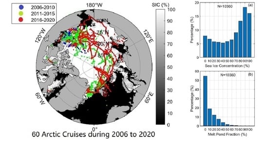
2.1. Ship-Based Observations

The ship-based observations of sea ice concentration (SIC) and melt pond fraction (MPF) in the Arctic from the Ice Watch Program (https://icewatch.met.no/; last access date: 12 July 2021) during 2006–2020 were used in this study. This dataset included 51 Arctic cruises, which are listed in Table 1. During 2006–2010, only one cruise was available every year, and the domain area during these years was in the Beaufort Sea. In the following years, at least two cruises were undertaken each year, and the cruise trajectories covered most regions of the Arctic Ocean, except for the thick multi-year area near the Canadian Arctic Archipelago (Figure 1a). Most of the cruises operated in summer, with some in the cold season. Sea ice concentration and melt pond fraction were observed every hour using the Arctic Shipborne Sea Ice Standardization Tool (ASSIST) (https://icewatch.met.no/assist; last access date: 12 July 2021), which follows the World Meteorological Organization’s (WMO, 1970) convention and is compatible with rules of Antarctic Sea Ice Processes and Climate (ASPeCt) [28]. Specifically, sea ice concentration (SIC) was estimated by professional scientists standing on the bridge of vessel as the sea ice percentage in a special region surrounding the vessel, with a diameter of 5 km for clear days and 1 km for foggy days. Melt pond fraction (MPF) was estimated as the melting pool percent of the sea ice in the observed region. Owing to our focus on melt ponds, only the observations between 1 June and 31 October were used, and a total of 5914 individual records from Ice Watch were available for our study.
During the 5th to 11th Chinese National Arctic Research Expedition (CHINARE) cruises in summer 2012 to 2020, the Icebreaker RV Xuelong I/II usually started her Arctic cruises through the Bering Strait in early July and finished in early October (Figure 1b). The traditional activity area was in the Chukchi Sea and the Beaufort Sea, which were visited every cruise. The other important Arctic seas, including the East Siberian Sea, Laptev Sea, Barents Sea, Norwegian Sea, and Greenland Sea, were also visited in several different years. In particular, the Icebreaker Xuelong passed through the Northeast Passage during summer 2012 and the Northwest Passage during summer 2017. In total, the ship-based observations from eight Xuelong I/II cruises were used in this study. During these voyages, the manual observations were conducted by professional researchers onboard the Xuelong. Sea ice concentration and melt pond fraction were recorded based on visual observations every half hour according to the guidance of the ASPeCt, which was similar to that used for the Ice Watch Program. Totally 4446 individual ship-based observations were made between 1 June and 31 October for our study. The ship-based observations from the Xuelong I/II were released by the National Arctic and Antarctic Data Center of China (https://www.chinare.org.cn/; last access date: 12 July 2021).
A total of 10,360 individual ship-based SIC and MPF observations were used in this study. The histograms are shown in Figure 2. Nearly half of the ship-based SICs were 80–100% (Figure 2a) and more than half of the ship-based MPFs were 0 (Figure 2b).

2.2. Satellite Products

The SSMIS onboard the Defense Meteorological Satellite Program’s (DMSP)-F17 satellite was launched in 2006. It is a polar orbiting conically scanning radiometer with a constant incidence angle of 53.1° and a swath width of about 1700 km. It has window channels near 19, 37, 91, and 150 GHz and sounding channels near 22, 50, 60, and 183 GHz. Here, we introduce three SIC products produced using different algorithms. All of the products are based on SSMIS data collections.
The SSMIS-NT sea ice concentration product used in this study was produced by NASA Goddard Space Flight Center using the NASA Team algorithm [29]. NT algorithm uses fixed tie-points. The released time series was updated daily, with a 25 km grid spacing and a start time of 1978, through a combination of the Scanning Multichannel Microwave Radiometer (SMMR) on the Nimbus-7 satellite and the SSMI sensors on the DMSP-F8, -F11, and -F13 satellites. It can be accessed from the NSIDC website https://nsidc.org/data/NSIDC-0051/versions/1 (last access: 12 July 2021).
The SSMIS-BT sea ice concentration product was generated using the Bootstrap Algorithm with daily varying tie-points, and it was produced by NASA Goddard Space Flight Center. The ocean tie points change each day (similar to the ice tie points) based on brightness temperatures for that day. The threshold for the lower limit for ice was relaxed to allow the retrieval of ice at an ice concentration of 10% [30]. The data are gridded on the SSM/I polar stereographic grid (25 × 25 km) and provided in two-byte integer format. The daily data for the north polar regions since 1978 are available from the NSIDC website https://nsidc.org/data/nsidc-0079/versions/3 (last access: 12 July 2021).
The SSMIS-OS sea ice concentration product (OSI-401-b) was produced using a combination of the Bristol algorithm and the Bootstrap algorithm by the Ocean and Sea Ice Satellite Application Facility (OSI SAF), which is hosted by Météo-France and is jointly operated by the Norwegian and Danish Meteorological Institutes. The ice concentrations were computed from the atmospherically corrected SSMIS brightness temperatures using a combination of state-of-the-art algorithms [31]. This algorithm used dynamical tie-points based on principal component analysis to determine clusters of sea ice and open water. It has been operational since 2005 and is updated daily. The spatial sampling of the product is 10 km. The dataset can be accessed at https://osi-saf.eumetsat.int/products/osi-401-b (last access: 12 July 2021).
The merged MODIS-AMSR2 sea-ice concentration dataset produced by the University of Bremen, Germany, was used as an independent source of the spatial 2D sea ice concentration [32]. This product was jointly retrieved from MODIS and ASI-AMSR2 data and has a very high resolution with a 1 km cell grid. The data are available operationally since 27 August 2019 during the start of the MOSAiC expedition. It is updated daily and can be downloaded from the website https://seaice.uni-bremen.de/sea-ice-concentration/modis-amsr2/ (last access: 12 July 2021).
The true color in the Moderate-resolution Imaging Spectroradiometer (MODIS) images was collected by the Terra and Aqua satellites. The spatial resolution is 250 m, and they cover the entire Arctic every day. These images can be ordered from the NASA Earthdata website (https://earthdata.nasa.gov; last access: 12 July 2021) and also can be download for free from the Worldview website (https://worldview.earthdata.nasa.gov/?p=arctic; last access: 12 July 2021). The advantages of the MODIS images are that they have a higher resolution than passive microwave products and their direct visualization can be used to distinguish sea ice distributions easily when the weather is clear. The disadvantage is that MODIS images are easily affected by clouds, and therefore, their availability is reduced by the frequent clouds in the Arctic summer.
The Multi-sensor Analyzed Sea Ice Extent (MASIE) was developed by the US National Ice Center (NIC), with support from the U.S. Navy and the National Oceanic and Atmospheric Administration (NOAA). This dataset was produced from multiple sources and is updated daily [33]. Its spatial resolution is 4 km. This product was used in this study as an independent source to validate the sea ice edges. MASIE can be downloaded for free from the NSIDC website (https://nsidc.org/data/masie; last access: 12 July 2021).
The satellite-retrieved melt pond fraction (MPF) datasets over the ice-covered Arctic Ocean, produced by the University of Bremen, were used in this study (https://seaice.uni-bremen.de/melt-ponds/; last access: 12 July 2021). The MPF datasets are available in three versions: MERIS MPF V1.0, MERIS MPF V1.5, and OLCI MPF V1.5. We used the OLCI MPF V1.5, which is based on the Ocean and Land Color Instrument (OLCI) onboard Sentinel-3 through MPD retrieval [34]. This dataset is gridded on a 12.5 km polar stereographic grid and is available for 2017 to 2020 [35].

2.3. Methods

The satellite products and ship-based observations had different spatial resolutions. For example, the SSMIS-based SIC products were updated daily, while the ship-based SIC was usually recorded every hour, of even every half hour. The grid cell for every single SIC value was 25 km for the SSMIS-NT and SSMIS-BT, while it was 10 km for the SSMIS-OS. The observation distance was 1–5 km under the different weather conditions for the ship-based SIC. To make the satellite product and ship-based observation records spatially comparable, the distances between each location of the ship-based observations and the grid cells of the satellite SIC were calculated. The grid cell with a minimum distance was selected as the corresponding satellite SIC for further comparisons. Considering that the speed of the icebreaker in the ice zone was generally around 15 km/h and the ship-based SIC observations were conducted every half to one hour, the distance between two adjacent observations was about 8 km; therefore, a three-point moving average was applied to the trajectories before the analysis and comparisons. In terms of temporal matching issues, the satellite SIC was averaged daily, and a pan-Arctic daily mean was also calculated to reduce the technical errors caused by the temporal and spatial variability, which was the method used by Zhao et al. [21] and Beitsch et al. [36].
For the satellite datasets, all the products were interpreted to a 25 km polar stereographic grid and used the same land mask before comparisons and calculations. MPFs in the in situ observations were subject to the ice-covered area around the ship, while in the OLCI dataset, they were gridded on a 12.5 km polar stereographic grid. We considered their transformation in this study.

3. Results

3.1. Spatial Inter-Comparisons of SSMIS-Based SIC

The spatial SIC distributions of the SSMIS-NT, SSMIS-BT, and SSMIS-OS on 25 July 2012 were chosen as a case study to illustrate their inter-comparisons in the early stage of the Arctic melt season. The large SIC differences in the marginal ice zone (MIZ), except for the central Arctic, are shown in Figure 3, and they represent a common condition for these SSMIS-based SIC products [21]. For example, in the Beaufort Sea toward the North Pole, the SSMIS-BT produced SICs of 70–100%, while the SSMIS-NT and SSMIS-OS produced SICs of 20–60%. The correlation coefficients of the spatial SIC distributions were 0.94 between the SSMIS-NT and SSMIS-OS, 0.95 between the SSMIS-BT and SSMIS-OS, and 0.84 between the SSMIS-NT and SSMIS-BT. The RMSE values were 12%, 16%, and 21%, between the SSMIS-NT and SSMIS-OS, the SSMIS-BT and SSMIS-OS, and the SSMIS-NT and SSMIS-BT, respectively.
When the sea ice edge retreated to 80° N in the minimum-extent month of September, the largest differences still occurred in the MIZ, and the SICs of the SSMIS-BT were 60–100%, while the SICs of the SSMIS-NT and SSMIS-OS were 20–80% (figures not shown). Further assessment of the SIC’s accuracy is described in Section 3.2. This assessment was conducted by comparing the products with ship-based SIC observations because the reported SSMIS-based SIC products usually underestimate the summer SIC [21].
When we investigated the zonal averaged SIC and the percentage of sea ice grid cells (SIC > 15%), the SSMIS-NT and SSMIS-OS were found to have smaller SICs than the SSMIS-BT at every single latitude on 25 July 2012 (Figure 4a). In the MIZ between 70° N and 75° N, the differences were large (up to 20%), while in the central Arctic north of 85° N, the differences were about 10%. However, the percentages of sea ice grid cells were nearly the same (Figure 4b), which indicates that these three SSMIS-based SIC products successfully distinguish sea ice grid cells from sea water grid cells, but they estimated sea ice concentration in the same sea ice grid cells differently. During the minimum-extent period in September, different estimations of the zonally averaged SIC were still discovered, mainly in the MIZ region, and the percentages of the sea ice grid cells were similarly close to each other (figures not shown).
The sea ice edges of the SSMIS-NT, SSMIS-BT, and SSMIS-OS, which are defined as the locations where SIC = 15%, were evaluated using MODIS images and the MASIE products. The trajectories of the Xuelong on 25 July and 24 August 2012 were also illustrated to investigate the efficiencies of the different sea ice products for use by icebreakers and commercial vessels in the ice regions. Figure 5a shows a case in the Chukchi Sea on 25 July 2012, where the three SSMIS-based SIC produced reasonable sea ice edges, but they failed to cover the sea ice tail near 170° W, 70° N, which was around 300 km in length and 100 km in width (red box in Figure 5a). Therefore, the SSMIS-based SICs failed to describe the details of the sea ice edges. The Icebreaker Xuelong was sailing from the Chukchi Sea toward the East Siberian Sea on 25 July 2012, bypassing a relative higher concentration region along the Russian coast.
On 24 August 2012, the Xuelong was seeking a route to approach the North Pole. As is shown in Figure 5, the three SSMIS-based SICs successfully detected the leading inside edge of the high concentration area near 120° E, 84° N, which was around 250 km in length and 50 km in width (red box in Figure 5b). The SSMIS-OS obtained the best illustration of the leading edge probably because of its high grid spacing. Therefore, the SSMIS-based SICs have the capacity to successfully detect the leading edge in the ice regions.
MODIS images were widely used to detect the sea ice extent and edges in the ice service due to its visibility and easy identification. On 24 August 2012 (Figure 5b), clouds covered most of the ice regions, making the ice detection difficult. In such cases, passive microwave products could play a critical role because they are free of the influence of clouds. As a product from multi-source satellites, the MASIE provided credible sea ice edges for both cases, and therefore, it is an efficient independent reference for sea ice edge recognition.

3.2. Comparisons of SSMIS-Based SICs with Ship-Based SICs

Figure 6 shows comparisons of the pan-Arctic daily mean values of the SSMIS-based SICs and ship-based SICs based on all 60 Arctic cruises conducted during 2006–2020. The correlation coefficients were 0.70, 0.82, and 0.83 between the ship-based SICs and the SSMIS-NT, SSMIS-BT, and SSMIS-OS SICs, respectively. The corresponding biases (RMSE) are −15% (27%), 3% (17%), and −9% (20%), which indicate that the SSMIS-NT and SSMIS-OS have negative biases, while the SSMIS-BT has a slight positive bias. Overall, the SSMIS-BT had the best fit, while the SSMIS-NT had the worst fit. The larger negative biases usually occurred in the low peak periods for the SSMIS-NT and SSMIS-OS SICs; while in the time periods with high SIC, a few positive biases existed for the SSMIS-BT SIC.
On a pan-Arctic daily mean scale, the histogram distribution of ship-based SIC exhibited a peak at 80%. However, the SSMIS-NT, SSMIS-BT, and SSMIS-OS had peaks at 80%, 100%, and 40%, respectively (Figure 7).
The relationship between the SSMIS-based SICs and the ship-based SIC along the trajectories of all 60 Arctic cruises were further studied using the scatter diagrams presented in Figure 8. The SSMIS-NT SIC had a correlation coefficient of 0.73 and a bias and RMSE of −15% and 24%, respectively. The underestimation in the high SIC range was obvious (Figure 8a). The relationship between the SSMIS-BT and the ship-based SIC had a correlation coefficient of 0.78, which was the highest for the three SSMIS-based products. The SSMIS-BT’s bias was 4%, which was the only positive bias, and its RMSE was 17%, which was the smallest. Based on the scatter plot, we found that the SSMIS-BT overestimated the high SIC range of 80–100% (Figure 8b). The SSMIS-OS had a high correlation coefficient of 0.77 and a negative bias of ‒7%. The RMSE of the SSMIS-OS was 19%, and it underestimated the values in the intermediate SIC range (Figure 8c). This large SIC mismatching phenomenon has also been observed in Antarctica when comparing the SICs produced by another passive microwave sensor (AMSR-E) with ship-based SICs following the ASPeCt rules [36].
In summary, the SSMIS-based SIC was evaluated on different scales (Table 2). Both comparisons revealed negative biases for the SSMIS-NT and SSMIS-OS SICs and a positive bias for the SSMIS-BT SIC. In addition, the SSMIS-BT had the smallest bias and RMSE.

3.3. Relationship between SSMIS-Based SIC Biases and Ship-Based MPF

The ship-based observed melt pond fractions (MPFs) for all the melt pond grid cells observed were used in this section for comparison with the SSMIS-based SIC biases calculated by subtracting the ship-based SICs. The results are shown in Figure 9. The ship-based MPFs are mainly distributed between 0 and 60%. The main biases were distributed within −50–10% for the SSMIS-NT, −30–10% for the SSMIS-BT, and −40–10% for the SSMIS-OS. Under higher MPF conditions, the SSMIS-based SICs generally exhibited larger biases, especially the SSMIS-OS SIC, with the largest slope being −0.36. The corresponding correlation coefficients were 0.16, 0.23, and 0.29 for the SSMIS-NT, SSMIS-BT, and SSMIS-OS, respectively, all of which reached the 99% significance level.
We used the degree of correlation between the SSMIS-based SIC biases and the ship-based MPFs as a measure of the algorithm’s sensitivity to melt ponds and used the obtained linear regression slope to estimate the differences between the actual and retrieved sea-ice concentrations. We used the ship-based MPF of 50% as a case study. The three products underestimated sea ice concentration by 20% (SSMIS-NT), 7% (SSMIS-BT), and 20% (SSMIS-OS) due to melt ponds. The underestimation decreased to about 10% for the SSMIS-NT when the MPF was zero. The SSMIS-BT SIC underestimation decreased to zero for a melt pond fraction of about 30%. For the SSMIS-OS, the underestimation decreased to zero when the MPF decreased to zero. When the MPF was less than 20%, the SSMIS-BT transitioned to overestimation, while the SSMIS-NT and SSMIS-OS still produced underestimations.

3.4. Spatial Influences of Melt Ponds on SSMIS SICs on the Basin Scale

In the above sections, we confirmed that large biases existed in the SSMIS-based SIC products. What should we do about this? Is it possible to correct the biases before we use these SIC products? We took the 2D sea ice concentrations on 6 September 2019 as an example of the summer Arctic to investigate the possibilities of correcting the biases caused by the melt ponds on the scale of an Arctic basin. The very high resolution (1 km) MODIS-AMSR2 SIC was used as an independent reference (Figure 10a). The OLCI MPF data from the University of Bremen were used to evaluate the spatial distribution of melt pond fraction (Figure 10b). The high SIC (80–100%) was distributed in the central Arctic along the Canadian Archipelago, and the low concentrations (20–60%) occurred in the marginal ice zone. In addition, the melt ponds commonly occurred in most regions of the sea ice ranging from 0 to 50%.
We took the relationships between the SSMIS-based SIC biases and the ship-based MPF obtained in Section 3.3 to assess the products’ sensitivity to melt ponds, following the method in Kern et al., 2016. The biases for every single grid cell were calculated when the MPF > 0%, and then, the original SICs were corrected using the calculated biases. The original SSMIS-NT SIC is shown in Figure 10c. The SIC was obviously underestimated in the Beaufort Sea, Greenland Sea, and East Siberia Sea. The corrected SSMIS-NT SIC (Figure 10d) shows improvements in the mean bias from −8% to −4% and in the RMSE from 20% to 17%. The SSMIS-BT was slightly improved in the MIZ region (Figure 10e,f), with the mean bias decreasing from 5% to −1%, but there was no change in the RMSE. For the SSMIS-OS, some of the low SIC regions were improved (Figure 10g,h) and the mean bias improved from −8% to −6%, while the RMSE decreased from 21% to 16% (Table 3).
When we investigated the zonal mean distribution of the SIC biases for the original and corrected products, it was clear that the SSMIS-NT SIC was significantly improved for latitudes of greater than 80° N (Figure 11a). The biases of the corrected SSIMS (red lines) were smaller for most of the latitude ranges. The standard deviation also narrowed when corrected. The bias of the SSMIS-BT was large at low latitudes, e.g., <85° N, but it became significantly smaller and close to zero at latitudes of greater than 85° N. The corrections had less influences on the SSMIS-BT SIC (Figure 11b). The bias improvement of the SSMIS-OS was obvious at latitudes greater than 80° N and was similar to that of the SSMIS-NT, i.e., the spread of the biases was smaller after the correction (Figure 11c).

4. Discussions

4.1. Uncertainties of Ship-Based Observations

Ship-based observations include some inevitable technological errors. (I) The ship-based observations along a trajectory may be reported with a smaller value because the vessels always try to avoid high ice concentration regions and chose a low ice concentration route when sailing in ice covered regions, which would lead to an underestimated SIC [37,38]. (II) Ship-based observations are conducted in the bridge of the vessel within a close distance, which is significantly smaller than the grid cell of every satellite product. Therefore, spatial mismatch probably occurs. (III) In terms of the temporal scale, the satellite SICs are the daily mean products, while the ship-based SICs are usually recorded every hour or half hour. The temporal mismatching may also introduce biases into the comparisons. (IV) Uncertainties may be introduced by changes in observers. Previous studies have reported 5–10% differences in total sea-ice concentration estimates based on observations of the same scene by different observers [39].
To minimize the influences of the uncertainties mentioned above in our comparisons, a three-point moving average was applied to the observations along the trajectories to match the satellite SIC and ship-based SIC in the spatial scale. Furthermore, we also used the daily mean along the trajectories and the pan-Arctic scale to match the comparisons on the temporal scale.

4.2. Uncertainties of OLCI MPF Products

Satellite remote sensing, ship-based observations, and aerial measurements are the common methods of retrieving melt pond fractions. Among them, the best quality and spatial coverage is provided by aerial measurements [34]. However, aerial measurements are difficult to conduct in the complicated environment of the Arctic, and the same is true for ship-based observations. The satellite-retrieved MPFs are easily obtained and have a large spatial coverage, but the algorithm may produce large uncertainties. A previous study involving a comparison of the satellite-retrieved MERIS MPF results and airborne-classified melt pond fractions reported an RMSE of 15% [34]. When the MERIS MPF products were compared to ship-based observations in the Arctic following the ASPeCt protocol, the results revealed an RMSE of 16% [40]. Another MODIS-based melt pond fraction was reported to have an RMSE of 4–11% based on comparison with independent melt-pond fraction observations [27].
In this study, the OLCI MPF products used to correct the three SSMIS-based SICs were evaluated using ship-based MPF observations from 60 Arctic cruises during 2017–2020. A weak correlation coefficient of 0.19 was found between the OLCI MPF and ship-based MPF, while the mean bias and RMSE were 14% and 17%, which indicate an obvious overestimation of the satellite-retrieved OLCI MPF products (Figure 12). Our assessment results are consistent with those of the previous studies mentioned above.
Clouds have an important influence on the OLCI MPF retrieval, because snow, sea ice and clouds have similar optical features in the available spectral range of OLCI 412.5–900 nm. A new cloud screening method was used to improve the cloud detection and comparison to the operational AATSR and MODIS cloud masks showed a considerable improvement in the detection of clouds over snow and sea ice, with about 5–10% false clear detections in the melting season [41].

4.3. The Influences of Tie-Points on Products’ Biases

Tie-points are typical signatures of 100% ice and open water which are used in the ice concentration algorithms as a reference. A possible reason for the differences is related to the tie-points used by the products. The SSMIS-NT algorithm uses fixed tie-points for each hemisphere, while the SSMIS-BT and SSMIS-OS algorithms use dynamic tie-points changed by date. The fixed tie-points cause great difficulty in distinguishing ice types during melt season and usually underestimate thin ice [29]. The dynamic tie-points are less sensitive to thin ice and layering of snow and ice, but are highly sensitive to changes in surface temperature, unlike the fixed tie-points [30]. For the SSMIS-OS product, dynamical tie-points are computed separately for the Bootstrap algorithm and the Bristol algorithm and both sets are used by the OSI SAF hybrid algorithm. Furthermore, the daily tie-point coordinates are combined into a 30-day running mean tie-point which is used in the further processing [31]. The inter-comparisons in this study indicated the treatment of tie-points largely influenced the accuracy of the products and the dynamic tie-points usually performed better than the fixed tie-points.

5. Conclusions

Sea ice concentrations based on passive microwave satellites are one of the most common products used for Arctic sea ice analysis, assimilation, modeling, and navigation due to their vast coverage, timely updating, and easy access. In this study, we evaluated three SSMIS-based SIC products: the NASA Team algorithm product (SSMIS-NT), the Bootstrap algorithm product (SSMIS-BT) by the NASA Goddard Space Flight Center, and the product combining the Bristol algorithm and the Bootstrap algorithm released by the OSI-SAF (SSMIS-OS). The ship-based SICs and MPF observations from 60 Arctic cruises by the Ice Watch Program and Chinese Xuelong I/II during 2006–2020 were used as independent data and a total of 10,360 individual observations were used.
The comparisons with the ship-based SIC observations suggest that the SSMIS-NT and SSMIS-OS underestimated the summer SIC, especially in the marginal ice zone. The SSMIS-NT had a mean bias of −15% and an RMSE of 24–27%, while the SSMIS-OS had a mean bias of −7–−9% and an RMSE of 19–20%. The SSMIS-BT overestimated the summer SIC, with a mean bias of 3–4% and an RMSE of 17%. When comparing the SICs in histogram form, the SSMIS-NT and SSMIS-OS overestimated the SIC in the low concentration areas (<20%) and underestimated the SIC in the high concentration areas (80–100%). The SSMIS-BT tended to treat the 80% SIC condition as completely ice covered (100% SIC). Further comparisons with the MODIS images and MASIE sea ice edge products revealed that the sea ice edges produced by the SSMIS-based SIC products successfully detected narrow leads (around 100 km scales) surrounded by a high ice concentration region, but they failed to describe the details of sea ice edges in the marginal ice zone.
The ship-based observed MPF was mainly less than 60%. The analysis in this study indicated that MPF had a potential influence on the SSMIS-based SIC retrieval. A relationship between the SIC biases and the ship-based MPF observations was established in this study. When melt pond fraction was 50%, the three products underestimated sea ice concentration by 20% (SSMIS-NT), 7% (SSMIS-BT), and 20% (SSMIS-OS) due to the melt ponds. These relationships were further used to correct the 2D distributions of the SSMIS-based SIC products, and the results were significantly improved. Taking 6 September 2019 as an example, the mean biases changed from −8% to −4% for the SSMIS-NT, from 5% to −1% for the SSMIS-BT, and from −8% to −6% for the SSMIS-OS after the corrections were conducted.
The tie-points used by the different products may relate to the biases. The SSMIS-NT algorithm uses fixed tie-points, while the SSMIS-BT and SSMIS-OS algorithms use dynamic tie-points. The fixed tie-points cause difficulty in distinguishing ice types during melt season and usually underestimate thin ice, indicating the potential to greatly influence the accuracy of the products and perform worse than fixed tie-points. Clouds influence the OLCI MPF retrieval, introducing about 5–10% false clear detections in the melting season, which may have influenced the accuracy of our analysis.
A similar investigation evaluating SIC retrieval algorithms in relation to melt ponds by comparing them with MODIS-retrieved SICs by Kern et al. in 2016 revealed an SIC underestimation between 14% and 26% for 100% with a MPF of 40% [23]. Previous studies on satellite-retrieved MPF reported RMSEs of 4–16% when compared with the MODIS-based MPF [27], the airborne-based MPF [34], and the ship-based MPF [40]. Our results are consistent with the previous studies.
In this study, the influence of melt ponds on SSMIS-based summer SICs in the Arctic were quantitatively assessed. In particular, the improvements from the melt pond correction provide a useful reference for sea ice research. Future attempts should focus on improving the SIC retrieval algorithm, for example, the detection and inclusion of melt pond fractions. When the SSMIS-based SICs are used for long-term sea ice analysis and model assimilation, their large summer biases and the influence of melt ponds should be kept in mind. More attempts to improve field observations and algorithms should be made in future because the accuracy of satellite SICs are essential for ship navigation, model assimilation, and climate change studies.

Author Contributions

Methodology, C.L.; data curation, H.G.; writing—original draft preparation, J.Z.; writing—review and editing, J.C.; visualization, Y.Y.; revision, Q.S.; supervision, J.Z. All authors have read and agreed to the published version of the manuscript.

Funding

This study was financially supported by the National Key Research and Development Program of China (2018YFC1407206; 2019YFE0105700-02).

Institutional Review Board Statement

Not applicable.

Informed Consent Statement

Not applicable.

Data Availability Statement

The ship-based observations from Ice Watch were available at https://icewatch.met.no/assist (last access date: 12 July 2021) and from Xuelong I/II were available at https://www.chinare.org.cn/ (last access date: 12 July 2021). SSMIS-NT and SSMIS-BT, and MASIE can be downloaded from NSIDC websites: https://nsidc.org/data/NSIDC-0051/versions/1 (last access: 12 July 2021), https://nsidc.org/data/nsidc-0079/versions/3 (last access: 12 July 2021), and https://nsidc.org/data/masie (last access: 12 July 2021), respectively. SSMIS-OS can be accessed at https://osi-saf.eumetsat.int/products/osi-401-b (last access: 12 July 2021). MODIS-AMSR2 and MPF can be downloaded from the University of Bremen websites: https://seaice.uni-bremen.de/sea-ice-concentration/modis-amsr2/ (last access: 12 July 2021) and https://seaice.uni-bremen.de/melt-ponds/ (last access: 12 July 2021), respectively. MODIS can be accessed from https://earthdata.nasa.gov (last access: 12 July 2021).

Acknowledgments

We would like to thank the University of Bremen for providing MODIS-AMSR2 dataset and DFG project REASSESS for providing the OLCI MPF products. We also thank NSIDC for providing SSMIS-NT, SSMIS-OS and MASIE products and OSI SAF for providing SSMIS-OS product. The same appreciations to Ice Watch and PRIC for providing the ship-based observations, to NASA for providing MODIS images. Finally, we truly appreciate reviewers for their valuable comments.

Conflicts of Interest

The authors declare no conflict of interest.

References

  1. Comiso, J.C.; Parkinson, C.L.; Gersten, R.; Stock, L. Accelerated decline in the Arctic sea ice cover. Geophys. Res. Lett. 2008, 35, L01703. [Google Scholar] [CrossRef] [Green Version]
  2. Haas, C.; Pfaffling, A.; Hendricks, S.; Rabenstein, L.; Etienne, J.L.; Rigor, I. Reduced ice thickness in Arctic Transpolar Drift favors rapid ice retreat. J. Geophys. Res. 2008, 35, L17501. [Google Scholar] [CrossRef] [Green Version]
  3. Nghiem, S.V.; Rigor, I.G.; Perovich, D.K.; Clemente-Colón, P.; Weatherly, J.W.; Neumann, G. Rapid reduction of Arctic perennial sea ice. Geophys. Res. Lett. 2007, 34, L19504. [Google Scholar] [CrossRef] [Green Version]
  4. Lei, R.B.; Xie, H.J.; Wang, J.; Leppäranta, M.; Jónsdóttir, I.; Zhang, Z.H. Changes in sea ice conditions along the Arctic Northeast Passage from 1979 to 2012. Cold Reg. Sci. Technol. 2015, 119, 132–144. [Google Scholar] [CrossRef]
  5. Xie, H.J.; Lei, R.B.; Wang, K.C.; Li, Z.; Zhao, J.; Ackley, S.F. Summer sea ice characteristics and morphology in the Pacific Arctic sector as observed during the CHINARE 2010 cruise. Cryosphere 2013, 7, 1057–1072. [Google Scholar] [CrossRef] [Green Version]
  6. Rodrigues, J. The rapid decline of the sea ice in the Russian Arctic. Cold Reg. Sci. Technol. 2008, 54, 124–142. [Google Scholar] [CrossRef]
  7. Stroeve, J.C.; Markus, T.; Boisvert, L.; Miller, J.; Barrett, A. Changes in Arctic melt season and implications for sea ice loss. Geophys. Res. Lett. 2014, 41, 1216–1225. [Google Scholar] [CrossRef]
  8. Cavalieri, D.J.; Gloersen, P.; Campbell, W.J. Determination of sea ice parameters with the Nimbus7 SMMR. J. Geophys. Res. 1984, 89, 5355–5369. [Google Scholar] [CrossRef]
  9. Comiso, J.C. Characteristics of Arctic Winter Sea ice from satellite multispectral microwave observations. J. Geophys. Res. 1986, 91, 975–994. [Google Scholar] [CrossRef]
  10. Comiso, J.C.; Cavalieri, D.; Parkinson, C. Passive microwave algorithms for sea ice concentrations. Remote Sens. Environ. 1997, 60, 357–384. [Google Scholar] [CrossRef]
  11. Comiso, J.C.; Steffen, K. Studies of Antarctic sea ice concentrations from satellite data and their applications. J. Geophys. Res. 2001, 106, 31361–31385. [Google Scholar] [CrossRef]
  12. Markus, T.; Cavalieri, D. An enhancement of the NASA team sea ice algorithm. IEEE Trans. Geosci. Remote 2000, 38, 1387–1398. [Google Scholar] [CrossRef] [Green Version]
  13. Comiso, J.C.; Parkinson, C.L. Arctic sea ice parameters from AMSR-E using two techniques and comparisons with sea ice from SSM/I. J. Geophys. Res. 2008, 113, C02S05. [Google Scholar] [CrossRef]
  14. Parkinson, C.L.; Comiso, J.C. Antarctic sea ice from AMSR-E from two algorithms and comparisons with sea ice from SSM/I. J. Geophys. Res. 2008, 113, C02S06. [Google Scholar] [CrossRef]
  15. Cavalieri, D.J.; Burns, B.A.; Onstott, R.G. Investigation of the effects of summer melt on the calculation of sea ice concentration using active and passive microwave data. J. Geophys. Res. 1990, 95, 5359–5369. [Google Scholar] [CrossRef]
  16. Steffen, K.; Schweiger, A. NASA team algorithm for sea ice concentration retrieval from defense meteorological satellite program special sensor microwave imager: Comparison with landsat satellite imagery. J. Geophys. Res. 1991, 96, 21971–21987. [Google Scholar] [CrossRef]
  17. Comiso, J.C.; Kwok, R. Surface and radiative characteristics of the summer arctic sea ice cover from multisensor satellite observation. J. Geophys. Res. 1996, 101, 28397–28416. [Google Scholar] [CrossRef]
  18. Fetterer, F.; Untersteiner, N. Observations of melt ponds on arctic sea ice. J. Geophys. Res. 1998, 103, 24821–24835. [Google Scholar] [CrossRef]
  19. Eicken, H.; Grenfell, T.C.; Perovich, D.K.; Richter-Menge, J.A.; Frey, K. Hydraulic controls of summer arctic pack ice albedo. J. Geophys. Res. 2004, 109, C08007. [Google Scholar] [CrossRef] [Green Version]
  20. Curry, J.A.; Schramm, J.L.; Ebert, E.E. Sea ice-albedo climate feedback mechanism. J. Climate 1995, 8, 240–247. [Google Scholar] [CrossRef]
  21. Zhao, J.C.; Zhou, X.; Sun, X.Y.; Cheng, J.J.; Hu, B.; Li, C.H. The inter comparison and assessment of satellite sea-ice concentration datasets from the arctic. J. Remote Sens. 2017, 21, 351–364. [Google Scholar] [CrossRef]
  22. Kern, S.; Lavergne, T.; Notz, D.; Pedersen, L.T.; Tonboe, R.T.; Saldo, R.; Sørensen, A.M. Satellite passive microwave sea-ice concentration data set intercomparison: Closed ice and ship-based observations. Cryosphere 2019, 13, 3261–3307. [Google Scholar] [CrossRef] [Green Version]
  23. Kern, S.; Rösel, A.; Pedersen, L.T.; Ivanova, N.; Saldo, R.; Tonboe, R.T. The impact of melt ponds on summertime microwave brightness temperatures and sea-ice concentrations. Cryosphere 2016, 10, 2217–2239. [Google Scholar] [CrossRef] [Green Version]
  24. Andersen, S.; Tonboe, R.; Kaleschke, L.; Heygster, G.; Pedersen, L.T. Intercomparison of passive microwave sea ice concentration retrievals over the high-concentration Arctic sea ice. J. Geophys. Res. 2007, 112, C08004. [Google Scholar] [CrossRef]
  25. Chen, Z.Q.; Liu, J.P.; Song, M.R.; Yang, Q.H.; Xu, S.M. Impacts of Assimilating Satellite Sea Ice Concentration and Thickness on Arctic Sea Ice Prediction in the NCEP Climate Forecast System. J. Climate 2017, 30, 8429–8446. [Google Scholar] [CrossRef]
  26. Kern, S.; Lavergne, T.; Notz, D.; Pedersen, L.T.; Tonboe, R. Satellite passive microwave sea-ice concentration data set inter-comparison for Arctic summer conditions. Cryosphere 2020, 14, 2469–2493. [Google Scholar] [CrossRef]
  27. Rösel, L.A.; Kaleschke, L.; Kern, S. Influence of melt ponds on microwave sensors’ sea ice concentration retrieval algorithms. In Proceedings of the IEEE International Geoscience and Remote Sensing Symposium (IGARSS), Munich, Germany, 22–27 July 2012. [Google Scholar]
  28. Worby, A.; Ian, A.; Vito, D. Technique for Making Ship-Based Observations of Antarctic Sea Ice Thickness and Characteristics; Australia Antarctic Division: Hobart, Australia, 1999.
  29. Cavalieri, D.; Parkinson, C.; Gloersen, P.; Zwally, H.J. Sea Ice Concentrations from Nimbus-7 SMMR and DMSP SSM/I-SSMIS Passive Microwave Data; NASA DAAC at the National Snow and Ice Data Center: Boulder, CO, USA, 1996. [Google Scholar] [CrossRef]
  30. Comiso, J.C. Bootstrap Sea Ice Concentrations from Nimbus-7 SMMR and DMSP SSM/I-SSMIS, Version 3. [Indicate Subset Used]; NASA National Snow and Ice Data Center Distributed Active Archive Center: Boulder, CO, USA, 2017. [Google Scholar] [CrossRef]
  31. Steinar Eastwood. Sea Ice Product User’s Manual OSI-401-a, OSI-402-a, OSI-403-a, Version 3.11; The European Organization for the Exploitation of Meteorological Satellites (EUMETSAT): Darmstadt, Germany, 2014. [Google Scholar]
  32. Ludwig, V.; Spreen, G.; Haas, C.; Istomina, L.; Kauker, F.; Murashkin, D. The 2018 North Greenland polynya observed by a newly introduced merged optical and passive microwave sea-ice concentration dataset. Cryosphere 2019, 13, 2051–2073. [Google Scholar] [CrossRef] [Green Version]
  33. Fetterer, F.; Savoie, M.; Helfrich, S.; Clemente-Colón, P. Multisensor Analyzed Sea Ice Extent—Northern Hemisphere (MASIE-NH), Version 1. [Indicate Subset Used]; National Snow and Ice Data Center: Boulder, CO, USA, 2010. [Google Scholar]
  34. Zege, E.; Malinka, A.; Katsev, I.; Prikhach, A.; Heygster, G.; Istomina, L.; Birnbaum, G.; Schwarz, P. Algorithm to retrieve the melt pond fraction and the spectral albedo of Arctic summer ice from satellite optical data. Remote Sens. Environ. 2015, 163, 153–164. [Google Scholar] [CrossRef] [Green Version]
  35. Istomina, L.; Marks, H.; Niehaus, H.; Huntemann, M.; Heygster, G.; Spreen, G. Retrieval of sea ice surface melt using OLCI data onboard Sentinel-3. In Proceedings of the AGU Fall Meeting, Online Everywhere, 1–17 December 2020. [Google Scholar]
  36. Beitsch, A.; Kern, S.; Kaleschke, L. Comparison of SSM/I and AMSR-E sea ice concentrations with ASPeCt ship observations around Antarctica. IEEE Trans. Geosci. Remote 2015, 53, 1985–1996. [Google Scholar] [CrossRef]
  37. Cicek, O.B.; Xie, H.; Ackley, S.F.; Ye, K. Antarctic summer sea ice concentration and extent: Comparison of ODEN 2006 ship observations, satellite passive microwave and NIC sea ice charts. Cryosphere 2009, 3, 1–9. [Google Scholar] [CrossRef] [Green Version]
  38. Worby, A.P.; Geiger, C.A.; Paget, M.J.; Van Woert, M.L.; Ackley, S.F.; DeLiberty, T.L. Thickness distribution of Antarctic sea ice. J. Geophys. Res. 2008, 113, C05S92. [Google Scholar] [CrossRef] [Green Version]
  39. Worby, A.P.; Comiso, J.C. Studies of the Antarctic sea ice edge and ice extent from satellite and ship observations. Remote Sens. Environ. 2004, 92, 98–111. [Google Scholar] [CrossRef]
  40. Istomina, L.; Heygster, G.; Huntemann, M.; Schwarz, P.; Birnbaum, G.; Scharien, R.; Polashenski, C.; Perovich, D.; Zege, E.; Malinka, A.; et al. Melt pond fraction and spectral sea ice albedo retrieval from MERIS data—Part 1: Validation against in situ, aerial, and ship cruise data. Cryosphere 2015, 9, 1551–1566. [Google Scholar] [CrossRef] [Green Version]
  41. Istomina, L.; Marks, H.; Huntemann, M.; Heygster, G.; Spreen, G. Improved cloud detection over sea ice and snow during Arctic summer using MERIS data. Atmos. Meas. Tech. 2020, 13. [Google Scholar] [CrossRef]
Figure 1. (a) Illustration of the trajectories of the 60 Arctic cruises used in this study, with blue denoting 2006–2010, green denoting 2011–2015, and red denoting 2016–2020. The background image is sea ice concentration on 1 July 2018. (b) The temporal distribution of the 60 Arctic cruises was 2006–2020. The different colors and line types represent the different vessels, which correspond to Table 1.
Remotesensing 13 03882 g001
Figure 2. The distribution of the ship-based observed sea ice concentration (SIC) (a) and melt pond fraction (MPF) (b) values for all 60 cruises.
Remotesensing 13 03882 g002
Figure 3. Inter-comparison of the spatial distributions of (a) SSMIS-NT, (b) SSMIS-BT, and (c) SSMIS-OS SIC on 25 July 2012.
Remotesensing 13 03882 g003
Figure 4. (a) The zonally averaged SIC and (b) the percentage of sea ice grid cells on 25 July 2012 for SSMIS-NT, SSMIS-BT, and SSMIS-OS.
Remotesensing 13 03882 g004
Figure 5. Comparisons of sea ice edges from the SSMIS-NT SIC (yellow dots), SSMIS-BT SIC (red dots), and SSMIS-OS (black dots): (a) in the Chukchi Sea on 25 July 2012 and (b) in the Central Arctic near the Laptev Sea on 24 August 2012. Sea ice edges are defined as the locations of 15% SIC. The background figures are the MODIS true color images for the corresponding day. The MASIE products were used as an independent reference (yellow lines). The trajectories of the Icebreaker Xuelong are denoted by the blue dots.
Remotesensing 13 03882 g005
Figure 6. Pan-Arctic daily mean ship-based SIC (blue lines), for the SSMIS-NT SIC (red lines in (a)), SSMIS-BT SIC (red lines in (b)), and SSMIS-OS SIC (red lines in (c)) corresponding to the ship-based observation locations for the specific cruise days. A seven-point moving average was applied to all the time series.
Remotesensing 13 03882 g006
Figure 7. Histogram for the (a) SSMIS-NT, (b) SSMIS-BT, and (c) SSMIS-OS and (d) ship-based SIC on a pan-Arctic daily mean scale.
Remotesensing 13 03882 g007
Figure 8. Scatterplots of the SSMIS-based SICs versus the ship-based SIC along all of the trajectories of the 60 Arctic cruises: (a) SSMIS-NT, (b) SSMIS-BT, and (c) SSMIS-OS. The black lines are 1:1 relationship lines and the red circles represent mean results for every 10% interval.
Remotesensing 13 03882 g008
Figure 9. Scatterplots of the SSMIS-based SIC biases versus the ship-based MPFs for all the melt pond grid cells observed: (a) SSMIS-NT, (b) SSMIS-BT, and (c) SSMIS-OS. The black lines are 1:1 relationship lines and the red circles represent mean results for every 10% interval.
Remotesensing 13 03882 g009
Figure 10. (a) The OLCI MPF, (b) MODIS-AMSR2 SIC, (c) original SSMIS-NT, (d) corrected SSMIS-NT SIC, (e) original SSMIS-BT, (f) corrected SSMIS-BT SIC, (g) original SSMIS-OS, and (h) corrected SSMIS SIC for 6 September 2019 as an example case.
Remotesensing 13 03882 g010
Figure 11. The zonal mean distribution of the SIC biases ± 1 STD for the three original (blue lines) and corrected (red lines) SSMIS-based products: (a) SSMIS-NT, (b) SSMIS-BT and (c) SSMIS-OS, for 6 September 2019, corresponding to Figure 10.
Remotesensing 13 03882 g011
Figure 12. (a) Scatter plot of the daily mean satellite-retrieved OLCI MPF versus the ship-based MPF during 2017–2020. The red lines are the corresponding linear fits. (b) Scatter plot of the MERIS retrieved MPF versus the airborne measured MPF for 7 June 2008, adopted from a previous study [34].
Remotesensing 13 03882 g012
Table 1. A list of the 60 Arctic cruises used in this study from Ice Watch and Xuelong I/II, including the cruise year, vessel names, flag country, and ship-based observation periods.
YearVessel NamesCountryPeriodYearVessel NamesCountryPeriod
2006Louis S. St. LaurentCanada5 Aug–14 Sep201650 let PobedyRussia11 Jul–13 Aug
2007Louis S. St. LaurentCanada26 Jul–31 AugLouis S. St. LaurantCanada22 Sep–16 Oct
2008Louis S. St. LaurentCanada17 Jul–20 AugMS ExpeditionCanada7 Jul–14 Jul
2009Louis S. St. LaurentCanada17 Sep–15 OctRV LanceNorway23 Aug–13 Sep
2010Louis S. St. LaurentCanada15 Sep–15 OctXuelongChina25 Jul–31 Aug
2011Louis S. St. LaurentCanada21 Jul–18 Aug201750 let PobedyRussia15 Jun–3 Jul
USCG HealyUSA15 Aug–28 SepLouis S. St. LaurentCanada6 Sep–5 Oct
2012Arctic SunriseGreenpeace5 Sep–12 SepPolarsternGermany27 May–11 Jul
RV LanceNorway18 Aug–11 SepRV LanceNorway19 May–23 May
Louis S. St-LaurentCanada1 Aug–8 SepXuelongChina2 Aug–7 Sep
OdenSweden15 Sep–25 Sep2018CCGS AmundsenCanada13 Jul–25 Jul
XuelongChina20 Jul–7 SepLouis S. St. LaurentCanada5 Sep–2 Oct
PolarsternGermany2 Aug–7 OctOdenSweden1 Aug–25 Sep
2013RV LanceNorway11 Aug–12 SepPolarsternGermany5 Sep–16 Oct
Louis S. St. LaurentCanada1 Aug–2 SepRV Kronprins HaakonNorway16 Aug–21 Aug
OdenSweden19 Aug–2 SepRV Kronprins HaakonNorway25 Aug–24 Sep
2014RV LanceNorway20 Feb–3 MarHealyUSA14 Sep–19 Oct
RV LanceNorway25 Aug–11 Sep50 let PobedyRussia12 Jul–17 Jul
Louis S St. LaurentCanada21 Sep–17 Oct50 let PobedyRussia23 Jul–27 Jul
PolarsternGermany6 Jul–3 Aug50 let PobedyRussia31 Jul–11 Aug
XuelongChina30 Jul–2 SepXuelongChina31 Jul–31 Aug
201550 let PobedyRussia20 Jul–31 Jul2019KV SvalbardNorway14 Aug–9 Sep
HealyUSA9 Aug–12 OctRV Kronprins HaakonNorway5 Aug–27 Aug
KV SvalbardNorway15 Jan–18 JanRV Kronprins HaakonNorway1 Sep–16 Sep
RV LanceNorway10 Jan–27 MarRV Kronprins HaakonNorway12 Nov–27 Nov
Louis S. St. LaurentCanada18 Sep–18 OctRV Kronprins HaakonNorway28 Nov–17 Dec
RV LanceNorway11 Apr–22 JunRV SikuliaqUSA7 Nov–27 Dec
RV LanceNorway25 Aug–9 Sep2020KV SvalbardNorway18 Jul–10 Aug
PolarsternGermany19 May–28 JunKV SvalbardNorway15 Oct–25 Nov
RV Kronprins HaakonNorway24 Aug–13 Sep
XuelongChina28 Jul–1 Sep
Table 2. The biases, RMSEs, and correlation coefficients (Corr.) of the three SSMIS-based products on two different scales, with different sample numbers.
ScalesDaily Mean for Pan-Arctic
(N = ~740)
Daily Mean Along Trajectories (N = ~2500)
Products
BiasRMSECorr.BiasRMSECorr.
SSMIS-NT−15%27%0.70−15%24%0.73
SSMIS-BT3%17%0.824%17%0.78
SSMIS-OS−9%20%0.83−7%19%0.77
Table 3. The correlation coefficients (Corr.), mean biases, and RMSEs of original and corrected 2D distributions of the SSMIS-based SICs for 6 September 2019, compared with the 2D distribution of the MODIS-AMSR2 SIC on that day.
SSMIS-NTSSMIS-BTSSMIS-OS
OriginalCorrectedOriginalCorrectedOriginalCorrected
Corr.0.770.780.790.760.720.79
Bias−8%−4%5%−1%−8%−6%
RMSE20%17%17%17%21%16%
Publisher’s Note: MDPI stays neutral with regard to jurisdictional claims in published maps and institutional affiliations.

