Remote Sensing Scene Image Classification Based on Dense Fusion of Multi-level Features

Abstract

For remote sensing scene image classification, many convolution neural networks improve the classification accuracy at the cost of the time and space complexity of the models. This leads to a slow running speed for the model and cannot realize a trade-off between the model accuracy and the model running speed. As the network deepens, it is difficult to extract the key features with a sample double branched structure, and it also leads to the loss of shallow features, which is unfavorable to the classification of remote sensing scene images. To solve this problem, we propose a dual branch multi-level feature dense fusion-based lightweight convolutional neural network (BMDF-LCNN). The network structure can fully extract the information of the current layer through 3 × 3 depthwise separable convolution and 1 × 1 standard convolution, identity branches, and fuse with the features extracted from the previous layer 1 × 1 standard convolution, thus avoiding the loss of shallow information due to network deepening. In addition, we propose a downsampling structure that is more suitable for extracting the shallow features of the network by using the pooled branch to downsample and the convolution branch to compensate for the pooled features. Experiments were carried out on four open and challenging remote sensing image scene data sets. The experimental results show that the proposed method has higher classification accuracy and lower model complexity than some state-of-the-art classification methods and realizes the trade-off between model accuracy and model running speed.

1. Introduction

At present, remote sensing images with high resolution have been applied to many fields such as remote sensing scene classification [1], hyperspectral image classification [2], change detection [3,4], geographic image, and land use classification [5,6], etc. However, remote sensing images’ complex spatial patterns and geographical structure bring great difficulties to image classification. Therefore, it is particularly important to understand the semantic content of remote sensing images effectively. The purpose of this study is to find a simple and efficient lightweight network model, which can accurately understand the semantics of remote sensing images and efficiently classify remote sensing scene images. In order to effectively extract image features, researchers have proposed many methods. Initially, manually made feature descriptors were used to extract image features, such as color histograms [7], texture descriptors [8], local binary mode [9], GIST [10], directional gradient histograms [11], bag-of-visual words (BOVW) [12], etc. Then, in order to solve the disadvantages brought by the method of manually extracting features, researchers proposed some unsupervised feature learning methods that can automatically extract shallow detail features from images, such as principal component analysis (PCA), sparse coding [13], autoencoders [14], Latent Dirichlet allocation [15], and probabilistic latent semantic analysis [16]. The above two feature extraction methods are very effective for the extraction of shallow image information. However, it is difficult to extract high-level features of images with these methods, which limits the improvement of classification accuracy. To overcome the drawbacks of these methods, researchers have proposed convolutional neural networks that are able to automatically extract significantly discriminative features from images [17,18,19,20,21,22,23,24,25,26,27,28,29,30]. Since then, the model based on convolution neural networks has become the mainstream method in the field of remote sensing scene image classification. With the development of convolution neural networks, a lightweight convolution neural network can achieve a balance between the speed of model operation and the accuracy of model classification. At present, lightweight networks have been applied to many tasks, including image classification, image segmentation, target detection [31], etc. SqueezeNet proposed the fire module, which divides the original standard convolution layer into an extrusion layer and expansion layer. The extruded layer consists of a continuous set of 1 × 1 convolution, and the extension layer is composed of a set of continuous 1 × 1 convolution and 3 × 3 convolution channels [32]. MobileNet, proposed by the Google team, has three versions: V1, V2, and V3. MobileNetV1 uses depthwise separable convolution to split the ordinary convolution into depthwise convolution and 1 × 1 convolution, which greatly reduces the number of network parameters and improves the accuracy to a certain extent [33]. MobileNetV2 proposed an inverse residual module and a linear bottleneck structure. This bottleneck structure was first subjected to the convolution of 1 × 1 for ascending dimension, then 3 × 3 depthwise separable convolution for feature extraction, and 1 × 1 convolution for dimension reduction [34]. MobileNet V3 adds the SE module [35] and searches the configuration and parameters of the network using the neural structure search [36]. ShuffleNet is a highly efficient convolution neural network architecture designed for mobile devices with limited computing power. The architecture uses two operations, group convolution and channel mixing, which greatly reduces computational cost compared with some advanced models with similar accuracy [37]. Wan et al. [38] proposed a lightweight convolution neural network for multiscale feature fusion recognition, which fuses shallow edge information of the network with deep semantic information to enhance the ability of feature representation and uses multiscale features for joint recognition. Bai et al. [39] proposed a novel and lightweight multiscale depthwise network (MSDWNet) with efficient spatial pyramid attention (ESPA) for remote sensing scene image classification. Li et al. [40] proposed a random multiscale mapping method to generate a multiscale and lightweight architecture for remote-sensing image recognition. The experimental results show that the multiscale network is more suitable than the single-scale network for extracting remote sensing scene image features. Shi et al. [41] proposed a two-branch fusion structure for remote sensing scene image classification, stacked by traditional convolution and depthwise separable convolution sequences. The dual branch structure can enhance feature information by fusing, but as the network deepens, it is difficult to extract critical information, and shallow information is also lost. To solve this problem, based on the dual branch structure and fully considering the information exchange between different hierarchical features, a dual branch multi-level feature dense fusion-based lightweight convolutional neural network (BMDF-LCNN) is proposed. Experiments show that the proposed method considerably improves computational speed compared to classification methods with the same or even fewer parameter quantities. Moreover, the proposed method can provide better classification accuracy and realize the balance of speed and classification performance.

To verify the effectiveness of this method, a large number of experiments were performed on four open and challenging remote sensing image scene datasets. The experimental results show that the classification accuracy of the proposed method is equivalent to or even better than that of some state-of-the-art classification methods with lower complexity. The main contributions of this study are as follows:

(1) Pooling can reduce the feature map size to reduce the computational load of the model, but it also results in the loss of some key features. To solve this problem, we propose a hybrid downsampling method, which compensates for the pooled features by using a convolution branch to achieve the minimum loss of critical information while downsampling. Experiments show that the hybrid downsampling method is helpful in improving the performance of the model.

(2) The pure bi-branching structure is difficult to extract the key features of the feature map with the deepening of the network. It also causes the loss of shallow features due to the deepening of the network, which is catastrophic for the classification of remote sensing scene images. To solve this problem, we propose a multi-level feature-intensive fusion structure based on dual branches. Each layer of the structure not only uses 3 × 3 depthwise separable convolution, 1 × 1 standard convolution, and Identity for feature extraction but also integrates with the features extracted by 1 × 1 standard convolution in the previous layer. Through the three branches of 3 × 3 depthwise separable convolution, 1 × 1 standard convolution, and identity, the information of the current layer can be fully extracted and fused with the features extracted by 1 × 1 standard convolution in the previous layer, which can avoid the loss of shallow information due to network deepening.

(3) A lightweight convolution neural network composed of shallow mixed downsampling structure and deep dual branch multi-level feature-intensive fusion structure is presented. A series of experimental results show that the proposed network is more suitable for remote sensing scene image classification.

The rest of this paper is as follows. In the second section, the proposed dual branch multi-level feature dense fusion-based lightweight convolutional neural network (BMDF-LCNN) is introduced in detail. In the third section, experiments and analysis are carried out and compared with some state-of-the-art methods to prove the superiority of the proposed method’s performance. The fourth section contains the conclusion.

2. Methods

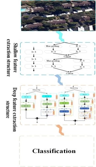
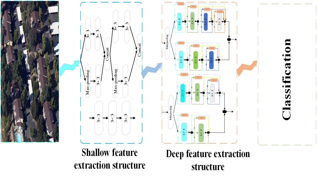
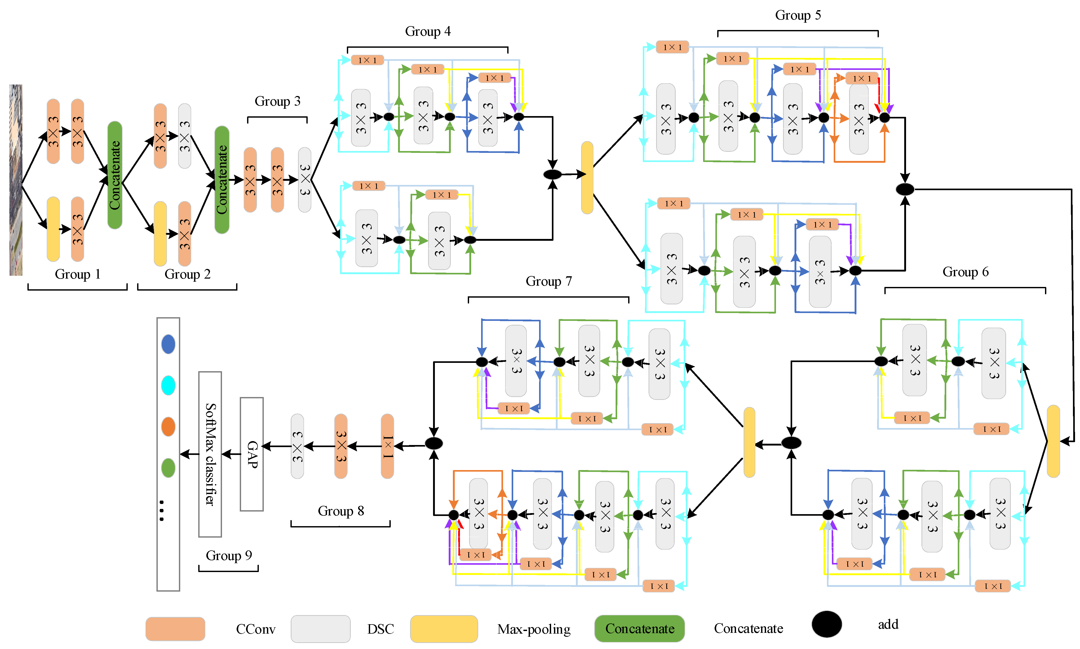
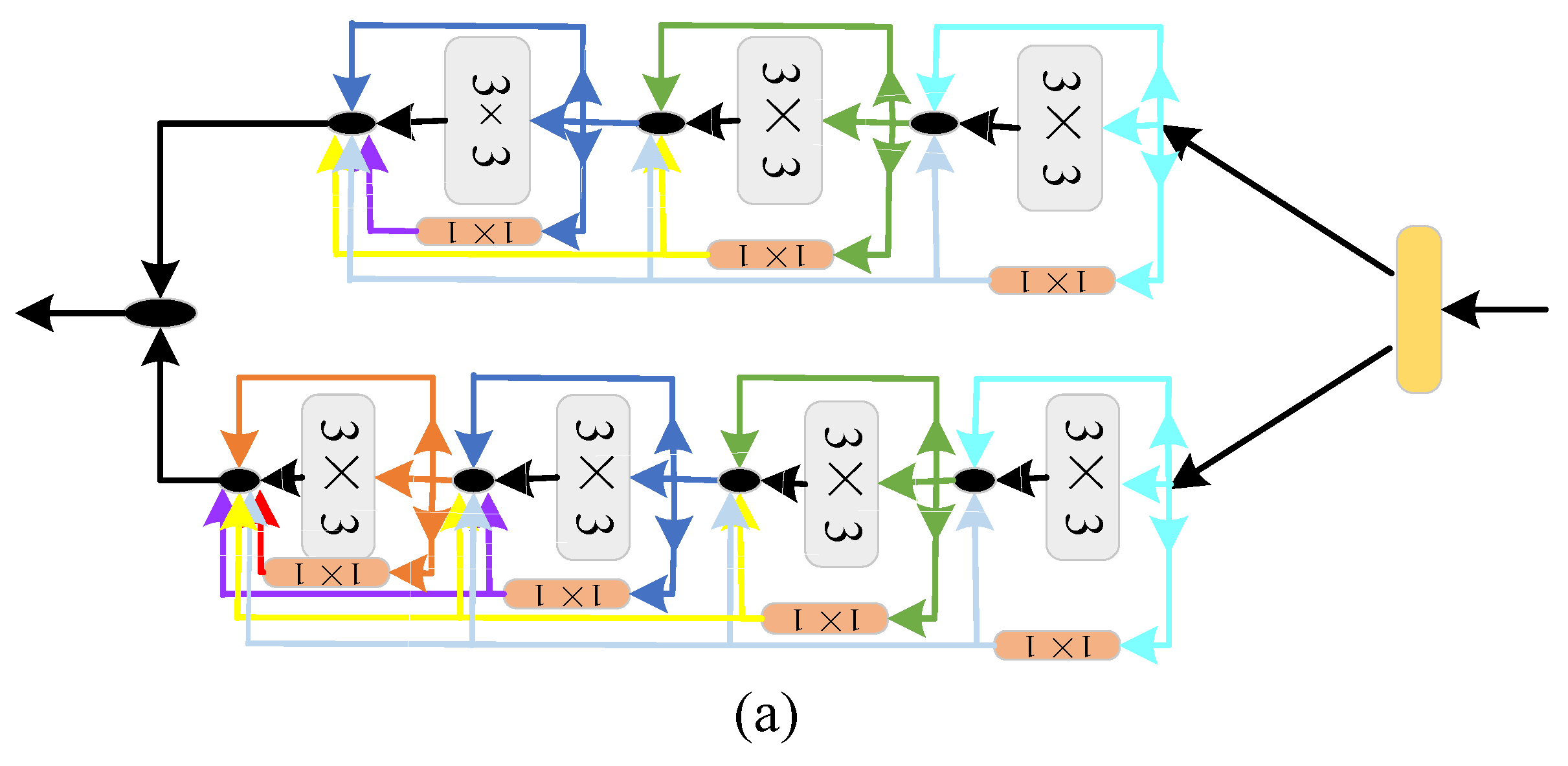
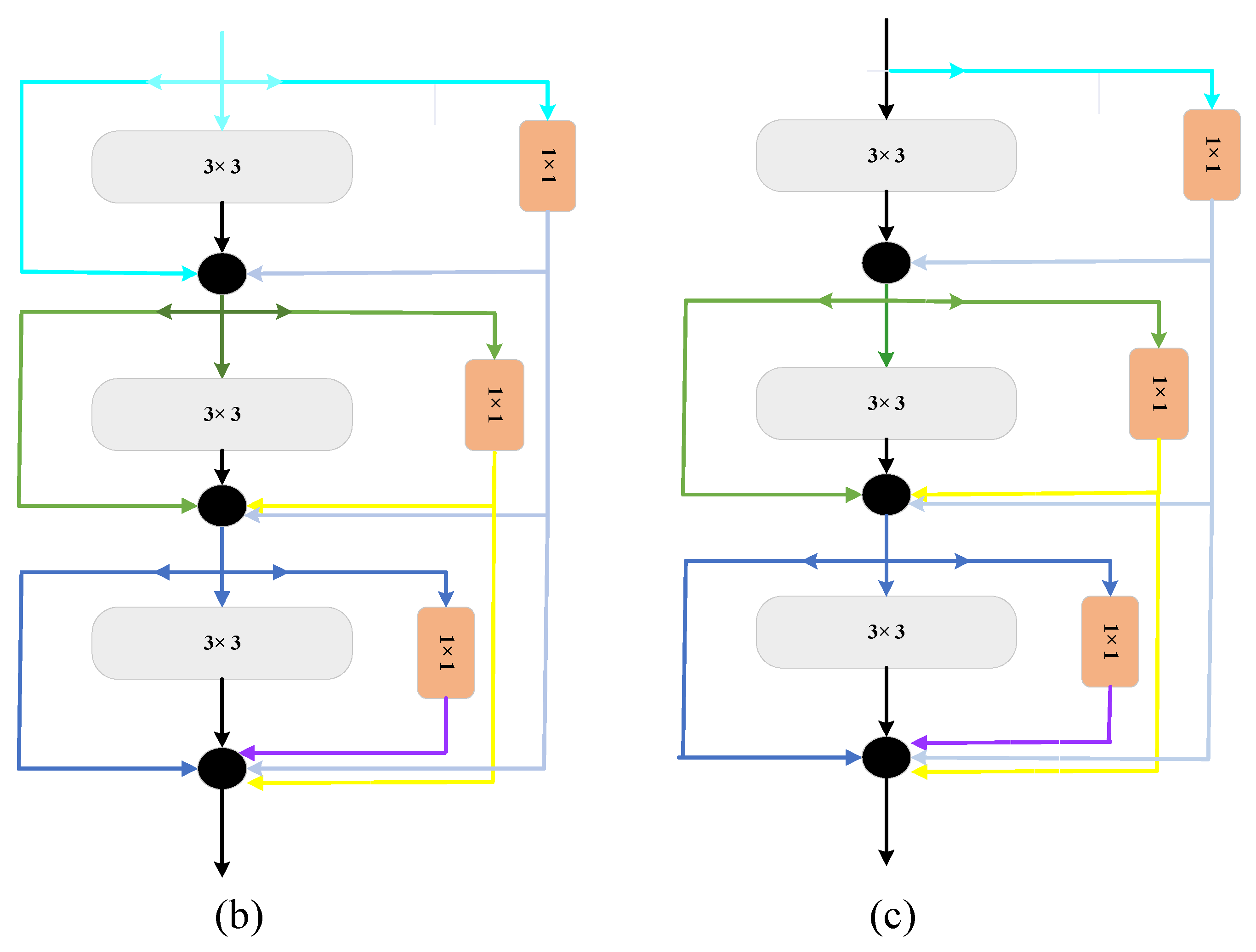
2.1. The Structure of the Proposed Method

The overall structure of the model is shown in Figure 1, which is divided into nine parts. In the first and second groups, we propose a feature extraction structure suitable for the shallow layers of the network (see Section 2.2 for the specific structure model). In the third group, the combination of standard convolution and depthwise separable convolution is adopted, and the maximum pool layer is used for downsampling to compress the spatial dimensions of the input images and reduce the risk of overfitting caused by irrelevant features. Groups 4 through 8 mainly extract representative features of remote sensing images. Groups 4 through 7 adopt the designed dual branch multi-level feature intensive fusion method to extract richer feature information. In Group 8, we used sequential 1 × 1 standard convolution, 3 × 3 standard convolution, and 3 × 3 depthwise separable convolution to extract deep-level features. On the basis of double branch fusion, the multi-level features are fully exchanged and fused, which not only improves the classification accuracy but also greatly improves the speed of the network and realizes the balance of accuracy and speed. In addition, in order to extract more features, the number of convolution channels in Groups 5 and 8 is widened to 256 and 512, respectively (see Section 3.2 for the specific channel number setting of other groups). Group 9 is used for classification, and the feature information obtained by the final fusion is utilized for calculating the probability of each scene category.

In deep feature extraction structures from Group 4 to Group 7, each layer can fully extract the information of the current layer through three branches of 3 × 3 depthwise separable convolution, 1 × 1 standard convolution, and Identity. In addition, by fusing the features extracted by 1 × 1 standard convolution with each previous layer, the shallow information loss due to network deepening can be effectively avoided. Using batch normalization (BN) [42] can reduce the dependence of the network on parameter initialization, make the training faster, and use a higher learning rate. In addition, compared with the natural image data set [43], the number of remote sensing images available for training is very small. To avoid possible over-fitting during training, L2 regularization is adopted after the cost function, which is:

$$J(\odot )=\frac{1}{2m}\left[{\displaystyle \sum _{i=1}^m(h_{\odot }(x^{(i)})}-y^{(i)}{)}^2+\gamma \left({\displaystyle \sum _{j=i}^n{\odot }_j^2}\right)\right]$$

(1)

The partial derivative of the above formula is:

$$\frac{\partial J(\odot )}{\partial {\odot }_j}=\frac{1}{m}{\displaystyle \sum _{i=1}^m(h_{\odot }}(x^{(i)})-y^{(i)})x_j^{(i)}+\frac{\gamma }{m}{\odot }_j$$

(2)

In the gradient descent algorithm, in order to converge as quickly as possible, the parameters will be updated along the negative direction of the gradient, so a negative sign is added before the partial derivative of Formula (2) and multiplied by a learning rate factor $\chi$ to obtain the final iteration weight parameter ${\odot }_j$, that is:

$${\odot }_j={\odot }_j-\chi ·\frac{\partial J(\odot )}{\partial {\odot }_j}$$

(3)

$${\odot }_j=\left(1-\frac{\chi \gamma }{m}\right){\odot }_j-\frac{\chi }{m}{\displaystyle \sum _{i=1}^m\left(h_{\odot }\left(x^{(i)}\right)-y^{(i)}\right)}{x}_j^{(i)}$$

(4)

where $\gamma$ is the regularization factor, we set it to 0.005, $J\left(\right)$ is the objective function, $x$ is the training sample, $y$ is the label corresponding to the training sample, and $h_{\odot }(x^{(i)})$ is the predicted value. As can be seen from Formula (4), each time the gradient is updated ${\odot }_j$ is multiplied by a factor $1-\frac{\chi \gamma }{m}$ less than 1, so as to attenuate the weight parameters and prevent overfitting. In Group 9, global average pooling [44] is used instead of the traditional full connection layer to avoid the overfitting of the full connection layer.

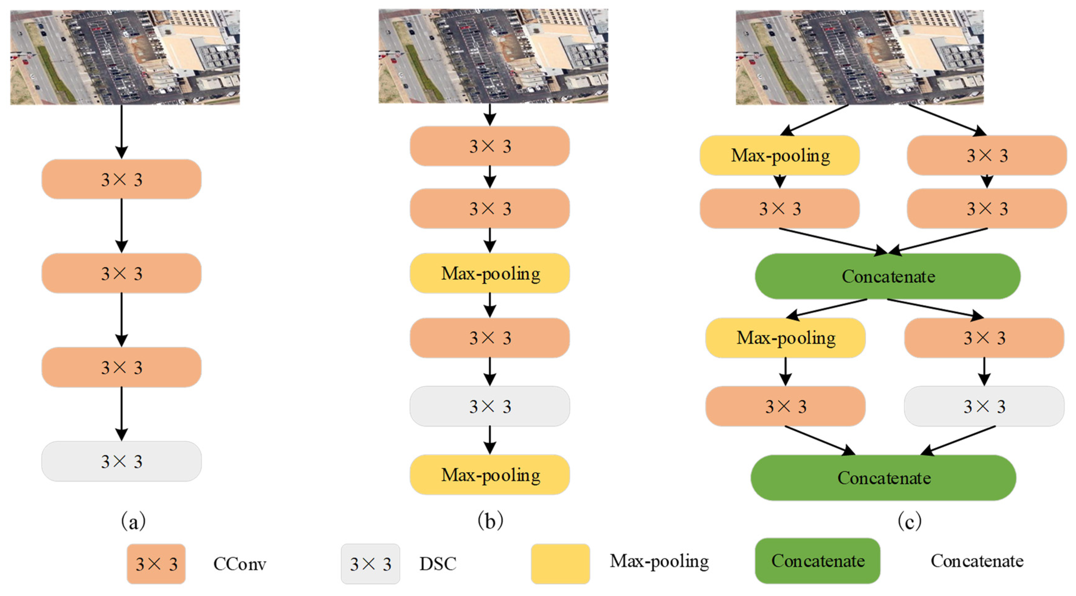
2.2. Shallow Feature Extraction Strategy

The first and second sets of downsampling structures are designed to extract the shallow features of the network. In the process of shallow feature extraction, the effect of downsampling on network performance is significant. Downsampling is the reduction of the convoluted feature map to a certain scale, reducing the spatial size of the image while preserving the main features of the image. The main methods of downsampling in deep convolution neural networks are maximum pooling downsampling and convolution downsampling. Pooling is a non-linear downsampling method that requires a deep convolution overlay. Generally speaking, it is better to use pooled downsampling for small convolution networks, but when the network is deep, multi-layer overlay convolution can learn better non-linear features from the training set. After analyzing the advantages and disadvantages of the two downsampling methods, a hybrid downsampling method based on pooling and convolution is proposed. The proposed hybrid downsampling structure is shown in Figure 2c. The pooling branch in this structure is used for downsampling, but pooling will lead to the loss of some key feature information, which is not conducive to extracting deep network features. Therefore, we use convolution to compensate for the lost features in another branch, which reduces the feature size and ensures the integrity of information to a great extent. Figure 2a,b are multi-layer convolution downsampling and pooling downsampling, respectively. In order to verify the performance of the proposed downsampling methods, the experimental comparisons of the three sampling methods are carried out in the third section.

2.3. Strategies to Optimize Time and Space Complexity

Figure 3a is the basic structure for optimizing time and space complexity. The structure is derived from the fusion of two branches with similar structures. For the sake of description, one of the branches is explained. According to the number of input and output channels in the first layer, two different structures are shown in Figure 3b,c. Each layer of the structure uses 3 × 3 depthwise separable convolution, 1 × 1 standard convolution, and Identity for feature extraction. Starting from the second layer, each layer of the structure not only uses 3 × 3 depthwise separable convolution, 1 × 1 standard convolution, and Identity for feature extraction but also integrates with the features extracted by 1 × 1 standard convolution in the previous layer. The process of dense fusion of multi-level features is as follows:

When the number of input and output channels of the first layer is the same ($C1=C2$), the structure is as shown in Figure 3b. The 3 × 3 branch of layer $i-1$ in this structure is represented by $\delta (BN(M^{(i-1)}\ast W^{(3)}))$, and the Identity branch of layer $i-1$, by $\delta (BN(M^{(i-1)}))$. Since each layer is fused with the 1 × 1 convolution branch of the previous layer starting from the second layer, we use ${\displaystyle \sum _{i=1}^i\delta (BN(M^{(i-1)}\ast W^{(1)}))}$ to represent the 1 × 1 convolution branch. The input of layer $i$ feature $M^{(i)}$ is $M^{(i-1)}$. In particular, we specify that the input of the first layer $M^{(1)}$ is $M^{(0)}$. The output features of each layer can be represented as:

$$M^{(i)}=\delta (BN(M^{(i-1)}\ast W^{(3)}))+\delta (BN(M^{(i-1)}))+{\displaystyle \sum _{i=1}^i\delta (BN(M^{(i-1)}\ast W^{(1)}))},i=1,2,3$$

(5)

Here, $BN$ is batch standardization; $\delta$ is the ReLU activation function; $W^{(3)}\in {ℝ}^{C_1\times C_2\times 3\times 3}$ represents the 3 × 3 depthwise separable convolution where the number of input channels is $C_1$ and the number of output channels is $C_2$. $W^{(1)}\in {ℝ}^{C_1\times C_2}$ represents the 1 × 1 convolution where the number of input channels is $C_1$ and the number of output channels is $C_2$.

When the number of input and output channels of the first layer is not the same ($C1\ne C2$), the structure is shown in Figure 3c. Only the first layer has no Identity branch, and the other layers have the same structure as in the case. The output feature of each layer is:

$$M^{(1)}=\delta (BN(M^{(0)}\ast W^{(3)}))+\delta (BN(M^{(0)}\ast W^{(1)})),i=1$$

(6)

$$M^{(i)}=\delta (BN(M^{(i-1)}\ast W^{(3)}))+\delta (BN(M^{(i-1)}))+{\displaystyle \sum _{i=1}^i\delta (BN(M^{(i-1)}\ast W^{(1)}))},i=2,3$$

(7)

The process of reducing model complexity is analyzed in detail as follows. The time complexity of a convolution neural network can be represented as:

$$T\sim O\left({\displaystyle \sum _{i=1}^L{M}_i^2}·K_i^2·C_{i-1}·C_i\right)$$

(8)

Here, $L$ denotes the number of convolution layers of the neural network, $M_i$ denotes the size of the output feature map of the $i$ convolution layer, $K_i$ denotes the convolution kernel size of the $i$ convolution layer, $i$ denotes the $i$ convolution layer of the neural network, and $C_{i-1}$ and $C_i$ denote the number of input and output channels $C_{in}$ and $C_{out}$ of the $i$ convolution layer of the neural network, respectively.

The spatial complexity of convolution neural networks is:

$$S\sim O\left({\displaystyle \sum _{i=1}^L{K}_i^2}·C_{i-1}·C_i+{\displaystyle \sum _{i=1}^L{M}_i^2}·C_i\right)$$

(9)

In Formula (9), the first summation expression represents the total weight parameters of all the layers with parameters in the model, and the second summation expression represents the size of the output feature map of each layer in the model.

2.3.1. Replace the Full Connection Layer with Global Average Pooling

Full Connection Layer is a special convolution layer whose convolution kernel size is the same as the input data size. The output feature map of each convolution kernel is a scalar, i.e., M = 1. The time and space complexity of the full connection layer are:

$$T\sim O(1^2·X^2·C_{in}·C_{out})$$

(10)

$$S\sim O(X^2·C_{in}·C_{out}+C_{out})$$

(11)

where X represents the size of the input image, M represents the size of the output feature map for each convolution kernel, K represents the size of the convolution kernel, $C_{in}$ and $C_{out}$ represent the number of input and output channels, respectively.

Formulas (10) and (11) show that the complexity of the full connection layer is related to the size of the input data. For global average pooling, the time and space complexity are:

$$T\sim O(C_{in}·C_{out})$$

(12)

$$S\sim O(C_{in}·C_{out})$$

(13)

As seen from (12) and (13), after using global average pooling, both time and spatial complexity are only related to the number of input-output channels, and the number of operations and parameters are greatly reduced.

2.3.2. Replacing Standard Convolution with Depthwise Separable Convolution

The standard convolution operation is to convolute all the channels of the input for each convolution kernel, and the depthwise separable convolution is that each convolution kernel acts on only a certain channel of the input, which reduces the complexity of the model.

The time complexity of standard convolution is:

$$T\sim O(M^2·K^2·C_{in}·C_{out})$$

(14)

The time complexity of depthwise separable convolutions is:

$$T\sim O(M^2·K^2·C_{in}+M^2·C_{in}·C_{out})$$

(15)

The number of parameters $P_{conv}$ of the standard convolution is:

$$P_{conv}=K·K·C_{in}·C_{out}$$

(16)

The number of parameters $P_{dsc}$ for the deep separable convolution is:

$$P_{dsc}=(K·K·C_{in}+C_{in}·C_{out})$$

(17)

The parameter number ratio of the depthwise separable and standard convolutions is:

$$P_{conv}/P_{dsc}=\frac{K·K·C_{in}+C_{in}·C_{out}}{K·K·C_{in}·C_{out}}=\frac{1}{C_{out}}+\frac{1}{K^2}$$

(18)

As can be seen from (14)–(18), when using a convolution kernel of 3 × 3, the parameter amount of the depthwise separable convolution is about $1/9$ that of the standard convolution. Therefore, the depthwise separable convolution is adopted, which can greatly reduce the number of parameters, effectively reduce the complexity of the model, and improve the running speed of the model.

2.3.3. Identity

In terms of network structure, the shallow network extracts simple and specific features. With the deepening of network structure, the extracted features become more complex and abstract. Since simple and abstract features can describe images from different aspects, the classification performance can be effectively improved through the information interaction between different hierarchical features. If Identity is not used, the classification of all images can only rely on complex features. After Identity is adopted, the shallow features can be retained, which can accelerate the running speed of the network.

3. Results

In this section, the proposed dual branching multi-level feature dense fusion method is comprehensively evaluated. Experiments are performed on four challenging datasets. The proposed BMDF-LCNN method is compared with some state-of-the-art classification methods. Experimental results demonstrate that the proposed method performs well with respect to various contrast indexes.

3.1. Dataset Settings

To prove the superiority of the proposed BMDF-LCNN method, the proposed BMDF-LCNN method and some state-of-the-art classification methods were compared experimentally in four datasets, the UC dataset [45], RSSCN dataset [46], AID dataset [47], and NWPU dataset [26]. The UC dataset is a remote sensing dataset of land use images from the USGS national map urban area imagery with a total of 2100 land use images in 21 categories, with 256 × 256 pixels per image. The RSSCN dataset is a remote sensing image dataset from Wuhan University with seven categories consisting of 2800 images, with 400 × 400 pixels per image. These images are sampled using different scales in different seasons and different weather conditions, making this dataset relatively challenging. The AID dataset is published jointly by Huazhong University of Science and Technology and Wuhan University. It has 10,000 remote sensing image datasets in 30 categories, with 600 × 600 pixels per image. The NWPU dataset is a remote sensing image dataset with 45 categories and 31,500 images created by Northern Polytechnic University, with 256 × 256 pixels per image. This dataset has the largest image size among the four datasets and the highest intra-class differences and inter-class similarities, which causes great challenges for classification tasks.

3.2. Setting of the Experiments

For the UC dataset, 80% of the images were randomly selected in each category as training data for model learning, and the remaining 20% of the images were used as test data to examine the performance of the model. For the RSSCN dataset, 50% of the images in each category were randomly selected as training data for model learning, and the remaining 50% were used as test data to verify model performance. For the AID dataset, 50% and 20% of the images were randomly selected in each category as training data for model learning, and the remaining images were used as test data to examine the performance of the model. For the NWPU45 dataset, 20% and 10% of the images in each category were randomly selected as training data for model learning, and the rest of the images were used as test data to verify the performance of the model.

The size of each convolution kernel is shown in Figure 1. Other settings are as follows:

In Group 1 and Group 2, the number of convolution filters is 32 and 64, respectively, with the first convolution step being 2 and the remaining convolution step being 1. To further extract high-level features, the number of convolution filters from Group 3 through Group 8 are 128, 128, 256, 256, and 512, respectively. Set the max-pooling size from Group 1 to Group 8 to 2 × 2, and the pool step is 2. All the steps of Group 3 through Group 8 are 1. To overcome the drawbacks of the small size of the training data and improve the generalization ability of the model, we used data enhancement to increase data diversity. The settings for data enhancement are as follows:

(1)

Multiplying all pixels of the input image by a scaling factor, which was set to 1/255, reduced the pixel value to between 0 and 1 and favored convergence of the model.

(2)

Select the appropriate angle to rotate the input image to change the orientation of the image content. Here, we chose a rotation angle of 0–60.

(3)

The input image was translated horizontally and vertically with a shift factor of 0.2.

(4)

The input image was randomly flipped to horizontal or vertical.

Furthermore, to reduce the risk of spillover of memory during training caused by excessive amounts of data, the input images were resized 256 × 256 with the bilinear interpolation method before training. Throughout the training process of the model, using an automatic learning rate reduction mechanism can reduce the learning rate according to the training situation and can quickly and accurately find the optimal model. The initial learning rate was set to 0.01. During the training process, the batch size was set to 16, and the momentum optimization algorithm was used to optimize the network for better and more stable convergence. Here we set the momentum factor to 0.9. The software used throughout the experiment was PyCharm. The final results were obtained by averaging the results of 10 experiments. The computer’s configuration is as follows: RAM: 16GB; Processor: AMD Ryzen 7 4800H with RadeonGraphics@2.90GHz; GPU: NVIDIAGeForceRTX2060 6G.

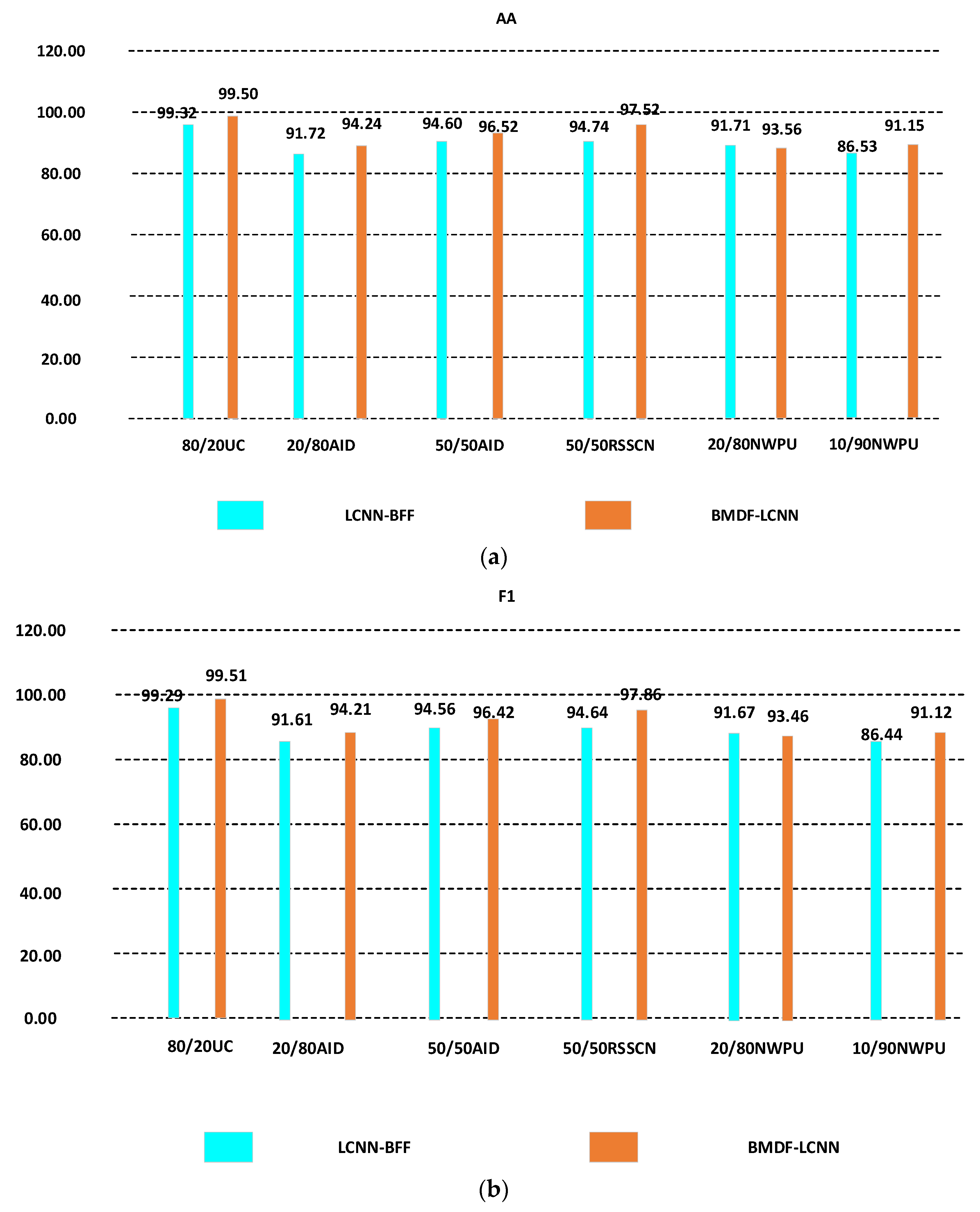
3.3. The Performance of the Proposed Model

To verify the advantages of the proposed BMDF-LCNN method over other methods, six evaluation indexes, including overall accuracy (OA), average accuracy (AA), Kappa coefficient (Kappa), confusion matrix, average training time (ATT), and weighting parameters were used to evaluate the proposed method comprehensively. OA represents the ratio of the correct number of classes to the total number of classes on all test sets, AA represents the ratio of the correct number of predictions for each class to the total number of classes and measures the quality of classification on each class by the proposed methods, ATT represents the average time spent training each image by the proposed methods, and F1 score can be regarded as the weighted average of model accuracy and recall rate. The higher the F1 value, the better the model. During the experiments, to ensure fairness of the experiments, all comparative experiments were conducted in the same experimental setting. Considering the proposed method is an improvement on the lightweight convolutional neural network-branch feature fusion (LCNN-BFF) method, in order to verify the advantages of the improved BMDF-LCNN method over the LCNN-BFF method, we use OA, AA, Kappa, and confusion matrix as evaluation indicators to compare the proposed method with LCNN-BFF method on four datasets: UC [45], RSSCN [46], AID [47], and NWPU [26]. The OA and Kappa results of the LCNN-BFF and BMDF-LCNN methods on six datasets are shown in

Table 1. Performance Comparison between LCNN-BFF and the Proposed Method.

	BMDF-LCNN		LCNN-BFF
	OA (%)	Kappa (%)	OA (%)	Kappa (%)
80/20UC	99.53	99.50	99.29	99.25
50/50RSSCN	97.86	97.50	94.64	93.75
20/80AID	94.46	94.26	91.66	91.37
50/50AID	96.76	96.24	94.62	94.41
10/90NWPU	91.65	90.65	86.53	86.22
20/80NWPU	93.57	93.42	91.73	91.54

.

As can be seen in Table 1, except for the 80/20UC dataset, both the OA and Kappa values of the proposed BMDF-LCNN method were elevated by more than 1% over those of the LCNN-BFF [41] method. The classification accuracy and Kappa value of the proposed BMDF-LCNN method on the UC dataset are close to 100%, which indicates that the method has better classification advantages on the UC dataset. Similarly, the BMDF-LCNN method has also achieved good classification results for the AID and NWPU datasets, with the most improvement on 10/90NWPU datasets, 5.12% higher classification accuracy, and 4.43% higher Kappa value than LCNN-BFF [41], indicating that the proposed method has better performance. Further, we use AP, F1, and confusion matrix as indicators to validate the advantages of the proposed method over other state-of-the-art classification methods.

The comparison of AA and F1 results between BMDF-LCNN and LCNN-BFF [41] is shown in Figure 4. Figure 4a shows that AA values obtained by BMDF-LCNN are superior to LCNN-BFF [41] in all comparison datasets. The highest performance improvement was achieved on 20/80AID, 50/50RSSCN, 20/80NWPU, and 10/90NWPU datasets, which were 2.52%, 2.78%, 1.85%, and 4.62% higher than LCNN-BFF, respectively.

As shown in Figure 4b, the F1 values obtained by the BMDF-LCNN method were also higher than that of LCNN-BFF. The four datasets, 20/80AID, 50/50RSSCN, 20/80NWPU, and 10/90NWPU, with the highest classification performance improvement, which was 2.6%, 3.22%, 1.79%, and 4.68% higher than LCNN-BFF [41], respectively.

Next, the confusion matrix is adopted to evaluate the performance of this method on four datasets, 20/80AID, 50/50RSSCN, 10/90NWPU, and 80/20UC. Each column in the confusion matrix represents the prediction category. Each line represents the actual category. The value on the diagonal line represents the probability value of the correct classification. The value outside the diagonal line indicates the probability of being wrongly classified as the current class.

From the results in Figure 5a, it can be seen that the classification accuracy of the BMDF-LCNN method for ‘Overpass’ and ‘Storage tanks’ is 95% on the 80/20UC dataset and 100% for other scenarios, which proves that this method has excellent performance on the UC dataset. Figure 5b shows that the BMDF-LCNN method achieves a classification accuracy of more than 96% for most scenes on the 50/50 RSSCN dataset. The recognition rate for ‘Industry’ is 94%. This is because the two scenes, ‘Industry’ and ‘Parking’, have mutually inclusive relationships, with the presence of cars in the industry and industry in the parking, which leads to easy confusion when classifying. Nevertheless, the BMDF-LCNN method still achieves high classification accuracy.

For the confusion matrix in Figure 6a, we can see that there are 20 categories on the 20/80AID datasets with classification accuracy above 95%, with the accuracy of ‘Forest’ and ‘Park’ at 100%. Five percent of the ‘Squares’ are misclassified as ‘Parks’, and five percent of the ‘Schools’ are misclassified as ‘Commercial’, mainly due to the high class similarity between ‘Parks’ and ‘Squares’, and ‘Schools’ and ‘Commercial’. In Figure 6b, on the 10/90NWPU datasets with high similarities between classes and intra-class differences, the classification accuracy of 39 classes is more than 90%, and that of ‘Chaparral’ and ‘Snowberg’ are 100%. Due to the high class similarity between ‘Palaces’ and ‘Churches’, 12% of palaces are misclassified as churches.

The above experiments fully demonstrate the validity of the proposed method through multiple evaluation indexes. The experimental results show that the dense fusion structure of two-branch and multi-layer features can significantly improve the classification accuracy and robustness of the network through the dense communication of different hierarchical features.

3.4. Comparison with Advanced Methods

In this section, in order to further verify the advantages of the proposed BMDF-LCNN method in model complexity and classification accuracy, the most advanced remote sensing scene classification methods proposed in the last two years were chosen and compared with the proposed BMDF-LCNN method on the UC [45], RSSCN [46], AID [47], and NWPU datasets [26]. These methods were evaluated using OA, AA, F1, the number of parameters, Kappa, ATT, and FLOPs as evaluation indexes.

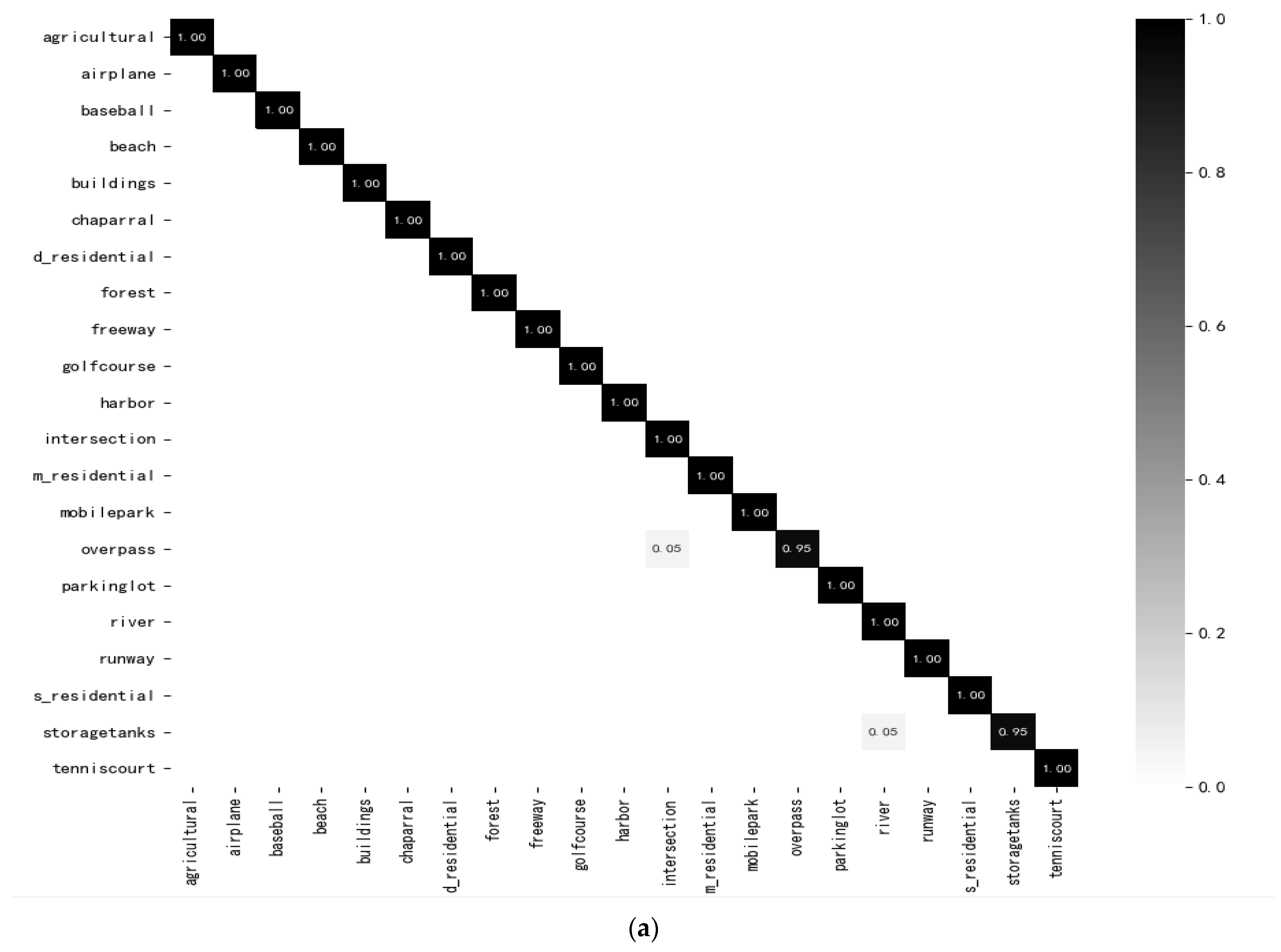
3.4.1. Experimental Results on UC-Merced Datasets

The comparison of the number of parameters, OA, AA, and F1 obtained by the proposed BMDF-LCNN method and that of the advanced methods are shown in

Table 2. Performance comparison of the proposed model with some state-of-the-art methods on UC Dataset.

The Network Model	OA (%)	AA (%)	F1	Number of Parameters
MRBF [14]	94.19 ± 1.5	94.25 ± 0.52	94.19 ± 0.26	89M
VWMF [23]	97.79	96.85	96.51	35M
VGG16-DF [27]	98.97	98.86	98.23	130M
BAFF [30]	95.48	95.69	94.96	130M
SF-CNN with VGGNet [32]	99.05 ± 0.27	98.89 ± 0.12	98.76 ± 0.15	130M
WSPM-CRC [33]	97.95	98.02	97.89	23M
Inception-v3-CapsNet [35]	99.05 ± 0.24	99.10 ± 0.15	99.05 ± 0.46	22M
ADFF [52]	98.81 ± 0.51	97.95 ± 0.92	97.84 ± 0.25	23M
MG-CAP(Bilinear) [53]	98.60 ± 0.26	98.50 ± 1.5	98.46 ± 0.18	45M
SCCov [48]	98.04 ± 0.23	98.35 ± 0.48	98.02 ± 0.29	6M
LiG with sigmoid kernel [51]	98.92	98.75	98.59	23M
GBNet + global feature [54]	98.57 ± 0.48	98.46 ± 0.43	98.32 ± 0.62	138M
FACNN [55]	98.81 ± 0.24	98.86 ± 0.19	98.76 ± 0.38	130M
SSRL [56]	94.05 ± 1.2	94.35 ± 0.09	94.05 ± 0.27	210M
VGG_VD16 + SAFF [57]	97.02 ± 0.78	96.56 ± 0.29	96.49 ± 0.21	15M
PANNet [49]	99.21 ± 0.18	98.26 ± 0.51	98.10 ± 0.27	28M
EfficientNet [58]	94.37	93.59	93.38	65M
EfficientNet-B3-Attn-2 [59]	99.21 ± 0.22	99.05 ± 0.19	98.98 ± 0.13	15M
Siamese [50]	94.29	93.56	93.37	21M
Contourlet CNN [50]	98.97	98.27	98.09	12.6M
BMDF-LCNN (Proposed)	99.53 ± 0.24	99.50 ± 0.15	99.51 ± 0.27	6M

. We can see in Table 2, for the UC dataset [45] with a training rate of 80%, the proposed method achieves a classification accuracy of 99.53%, which exceeds all the comparison methods. This indicates that the dense fusion module with two branches and multi-layers can significantly improve classification accuracy. Inception-v3-CapsNet [35], SF-CNN with VGGNet [32], SCCov [48] and PANNet [49] all achieve more than 99% classification accuracy. However, these four methods have a large number of parameters and do not have a good trade-off between the complexity of the model and the classification accuracy. The parameters of SCCov [48] are only 6M, which is the same as that of the proposed BMDF-LCNN method. However, the accuracy of SCCov [48] is only 98.04%, which is 1.49% lower than the proposed method. The F1 score of the proposed method is 99.51%, 1.49% higher than the lightweight method SCCov [48] and 1.42% higher than Contourlet CNN [50]. In addition, the Kappa values of the proposed methods are compared with those of the most advanced methods on the UC dataset [45], and the results are shown in

Table 3. Comparing the Kappa values of the proposed model with some advanced methods on the UC dataset.

The Network Model	Year	Kappa (%)
R.D [13]	2019	94.50
LiG with sigmoid kernel [51]	2020	97.63
EfficientNet [58]	2020	92.37
SE-MDPMNet [34]	2019	97.74
Fine-tune MobileNet [34]	2019	96.92
Siamese [50]	2019	94.00
Contourlet CNN [50]	2020	97.81
BMDF-LCNN (Proposed)	2021	99.50

. As shown in Table 3, the Kappa value of the proposed BMDF-LCNN method is 99.50%, 1.69% higher than that of Contourlet CNN [50], 1.87% higher than that of LiG with sigmoid kernrl [51], and 1.76% higher than that of SE-MDPMNet [34]. The comparison of the above data shows that the proposed BMDF-LCNN method can provide better classification performance.

To verify the strong immediacy of the proposed method, the proposed BMDF-LCNN method and several state-of-the-art methods were experimentally contrasted on UC datasets [45] under the same configuration conditions. The ATT comparison results are shown in

Table 4. The average time between the proposed model and some advanced methods for image processing.

The Network Model	ATT(s)
GBNet [54]	0.053
GBNet + global feature [54]	0.039
Siamese [50]	0.052
Siamese [50]	0.048
BMDF-LCNN (Proposed)	0.017

. From Table 4, we can see that the ATT of the proposed method is 0.017 s, which saves 0.035 s, 0.031 s to process an image with the two methods in [54] and saves 0.036 s and 0.022 s to process an image with the two methods in [50]. This further verifies the effectiveness of the method.

3.4.2. Experimental Results on RSSCN Datasets

Table 5. Performance comparison of the proposed model with some advanced methods on RSSCN datasets.

The Network Model	Year	OA (%)	AA (%)	F1	Number of Parameters
VWMF [23]	2019	89.10	88.96	88.69	35 M
WSPM-CRC [33]	2019	93.60	94.01	93.60	23 M
SPM-CRC [33]	2019	93.86	93.79	93.75	23 M
VGG16 + SVM [47]	2017	87.18	87.09	86.95	130 M
ADFF [52]	2019	95.21 ± 0.50	95.35 ± 0.67	94.87 ± 0.56	23 M
Two-stage deep feature fusion [60]	2018	92.37 ± 0.72	92.09 ± 0.53	92.35 ± 0.45	18 M
Fine-tune MobileNet [34]	2019	94.71 ± 0.15	93.52 ± 0.25	94.59 ± 0.19	3.5 M
SE-MDPMNet [34]	2019	92.46 ± 0.66	93.08 ± 0.42	92.46 ± 0.26	5.17 M
EfficientNet-B3-Attn-2 [59]	2021	96.17 ± 0.23	95.68 ± 0.35	95.53 ± 0.76	15 M
Contourlet CNN [50]	2020	95.54 ± 0.17	95.62 ± 0.26	95.06 ± 0.62	12.6 M
BMDF-LCNN (Proposed)	2021	97.86 ± 0.25	97.52 ± 0.10	97.86 ± 0.19	6 M

lists the comparison results of OA, AA, F1 scores and the number of parameters between the proposed method and the comparison method. It can be seen that the classification accuracy of this method is the highest. The OAs of the proposed methods are 2.32%, 2.65%, 5.40%, and 1.69% higher than that of Contourlet CNN [50], ADFF [52], SE-MDPMNet [34], and EffecientNet-B3-Attn-2 [59], respectively. The AAs of the proposed methods are 1.9%, 2.17%, 4.44%, and 1.99% higher than that of Contourlet CNN [50], ADFF [52], SE-MDPMNet [34], and EffecientNet-B3-Attn-2 [59], respectively. Moreover, compared with other methods, the proposed method has the least number of parameters, which accounts for only 4.61% of the parameters of VGG16+SVM [47], and 26.09% of the parameters of SPM-CRC [33], WSPM-CRC [33], and ADFF [52]. The F1 score of the proposed method is also the highest among all comparison methods. These indicators verify that the proposed network model has good classification performance.

3.4.3. Experimental Results on AID Datasets

The comparison results between the proposed BMDF-LCNN method and the most advanced method are listed in

Table 6. Performance comparison of the proposed model with some advanced methods on AID datasets.

The Network Model	OA (20/80) (%)	AA (20/80) (%)	OA (50/50) (%)	AA (50/50) (%)	Number of Parameters
BAFF [30]	91.23	90.65	93.56	93.42	130 M
VGG16-CapsNet [35]	91.63 ± 0.19	91.26 ± 0.59	94.74 ± 0.17	94.65 ± 0.36	22 M
MG-CAP(Bilinear) [53]	92.11 ± 0.15	92.28 ± 0.25	95.14 ± 0.12	95.26 ± 0.24	130 M
SCCov [48]	91.10 ± 0.15	91.35 ± 0.16	93.30 ± 0.13	93.45 ± 0.49	6 M
GBNet [54]	90.16 ± 0.24	89.94 ± 0.27	93.72 ± 0.34	93.68 ± 0.56	18 M
GBNet + global feature [54]	92.20 ± 0.23	91.87 ± 0.36	95.48 ± 0.12	94.97 ± 0.16	138 M
FACNN [55]	90.87 ± 0.53	91.05 ± 0.48	95.45 ± 0.11	95.62 ± 0.19	25 M
VGG_VD16 + SAFF [57]	90.25 ± 0.29	90.25 ± 0.68	93.83 ± 0.16	93.76 ± 0.28	15 M
InceptionV3 [62]	93.27 ± 0.17	94.05 ± 0.49	95.07 ± 0.22	95.38 ± 0.17	45.37 M
ResNet50 [62]	92.39 ± 0.15	91.69 ± 0.72	94.69 ± 0.19	95.02 ± 0.26	25.61 M
VGG19 [62]	87.73 ± 0.25	87.80 ± 0.16	91.71 ± 0.42	91.54 ± 0.65	19 M
EfficientNet [58]	86.56 ± 0.17	87.06 ± 0.15	88.35 ± 0.16	88.56 ± 0.53	65 M
LiG with RBF kernel [61]	94.17 ± 0.25	94.05 ± 0.52	96.19 ± 0.28	96.27 ± 0.39	2.07 M
Fine-tune MobileNetV2 [34]	94.13 ± 0.28	94.20 ± 0.18	95.96 ± 0.27	95.06 ± 0.28	10 M
MSDFF [63]	93.47	93.56	96.74	96.46	15 M
BMDF-LCNN (proposed)	94.46 ± 0.15	94.24 ± 0.10	96.76 ± 0.18	96.52 ± 0.23	6 M

. When the training ratio is 20%, the overall classification accuracy of the proposed method reaches 94.46%, which is 0.29% and 0.33% higher than that of LiG with RBF kernel [61] and that of Fine-tuneMobileNetV2 [34], respectively. The average accuracy of the proposed method is 94.24%, which is 2.89% and 0.19% higher than the lightweight methods SCCov [48] and LiG with RBF kernel [61], respectively. When the training ratio is 50%, the proposed method has the highest overall classification accuracy, which is 96.76%, which exceeds the accuracy of all the comparison methods. This accuracy is 1.31% higher than that of FACNN [55], 0.57% higher than that of LiG with RBF kernel [61], and 0.8% higher than that of Fine-tune MobileNetV2 [34]. Compared with the lightweight networks SCCov [48] and VGG_VD16 + SAFF [57], the average classification accuracy of the proposed method is improved by 3.07% and 2.76% respectively. This proves that our method can extract the features of images more effectively and understand the semantics of images more accurately. As far as the weight parameters are concerned, the weight parameters of the proposed method are 6M, slightly higher than that of LiG with RBF kernel [61], but our method can provide higher classification accuracy than LiG with RBF kernel [61].

The Kappa values of the proposed BMDF-LCNN method are compared with those of other methods, as shown in

Table 7. Comparison of Kappa results between the proposed model and other advanced methods on the AID dataset.

The Network Model	OA (50%)	Kappa (%)
VGG19 [62]	91.71	90.06
ResNet [62]	94.69	93.47
InceptionV3 [62]	95.07	93.91
EfficientNet [58]	88.35	87.21
LiG with RBF kernel [61]	96.19	94.33
Fine-tune MobileNet V2 [34]	95.96	94.83
BMDF-LCNN (Proposed)	96.76	96.24

. It can be seen that the Kappa values of the proposed method are 96.24%, 1.91% higher than that of LiG with RBF kernel [61] and 1.41% higher than that of Fine-tune MobileNet V2 [34].

3.4.4. Experimental Results on NWPU Dataset

Experiments were carried out on the NWPU data set. The comparison results between the proposed BMDF-LCNN method and some of the most advanced methods are shown in

Table 8. Performance comparison of the proposed model with some advanced methods on the NWPU dataset.

The Network Model	OA (10/90) (%)	AA (10/90) (%)	OA (20/80) (%)	AA (20/80) (%)	Number of Parameters	Year
R.D [13]	89.36	89.05	91.03	90.68	20 M	2019
VGG16-CapsNet [35]	85.08 ± 0.13	85.12 ± 0.22	89.18 ± 0.14	89.32 ± 0.19	22 M	2019
MG-CAP with Bilinear [53]	89.42 ± 0.19	89.06 ± 0.16	91.72 ± 0.16	90.95 ± 0.33	45 M	2020
SCCov [48]	84.33 ± 0.26	83.56 ± 0.48	87.30 ± 0.23	97.41 ± 0.53	6 M	2020
LiG with sigmoid kernel [51]	90.19 ± 0.11	89.57 ± 0.36	93.21 ± 0.12	93.05 ± 0.15	23 M	2020
VGG_VD16 + SAFF [57]	84.38 ± 0.19	84.23 ± 0.23	87.86 ± 0.14	88.03 ± 0.10	15 M	2021
VGG19 [62]	81.34 ± 0.32	81.02 ± 0.64	83.57 ± 0.37	83.69 ± 0.23	19 M	2020
Inception V3 [62]	85.46 ± 0.33	84.87 ± 0.15	87.75 ± 0.43	86.25 ± 0.45	45.37 M	2020
ResNet50 [62]	86.23 ± 0.41	85.73 ± 0.28	88.93 ± 0.12	88.42 ± 0.16	25.61 M	2020
EfficientNet [58]	78.57 ± 0.15	78.42 ± 0.18	81.83 ± 0.15	81.58 ± 1.19	65 M	2020
LiG with RBF kernel [61]	90.23 ± 0.13	89.28 ± 0.32	93.25 ± 0.12	92.82 ± 0.64	2.07 M	2020
MSDFF [63]	91.56	90.86	93.55	92.76 ± 0.35	15 M	2020
Contourlet CNN [50]	85.93 ± 0.51	86.05 ± 0.26	89.57 ± 0.45	89.08 ± 0.25	12.6 M	2020
BMDF-LCNN (Proposed)	91.65 ± 0.15	91.15 ± 0.10	93.57 ± 0.22	93.56 ± 0.35	6 M	2021

. In Table 8, when the training ratio is 10%, the overall classification accuracy of the proposed method reaches 91.65%, which is 1.42% higher than that of LiG with RBF kernel [61] and 1.46% higher than that of LiG with sigmoid kernel [51]. Compared with the lightweight networks SCCov [48] and LiG with RBF kernel [61], the average classification accuracy of the proposed method is improved by 7.59% and 1.87% respectively. When the training ratio is 20%, the overall classification accuracy is 0.32%, which is 0.36% and 0.02% higher than that of LiG with RBF kernel [61], LiG with sigmoid kernel [51], and MSDFF [63], respectively. The average accuracy of the proposed method is 93.56%, which is 4.48% and 0.8% higher than the lightweight methods Contourlet CNN [50] and MSDFF [63], respectively. In terms of parameters, compared with LiG with RBF kernel [61] with small parameters, when the training ratio is 10%, the classification accuracy of the proposed method is improved by 1.42%, and when the training ratio is 20%, the classification accuracy of the proposed method is improved by 0.32%. Compared with SSCov [48] with the same parameters, when the training ratio is 10%, the classification accuracy of the proposed method is improved by 7.32%, and when the training ratio is 20%, the classification accuracy of the proposed method is improved by 6.27%. Experimental results show that the proposed method has better classification performance and fewer parameters, which is very suitable for mobile devices.

The comparison of Kappa values of different methods is shown in

Table 9. Comparison of Kappa values between the proposed method and some advanced methods on 20% NWPU45 dataset.

The Network Model	OA (20%)	Kappa (%)
VGG19 [62]	83.57	82.17
ResNet [62]	88.93	87.61
InceptionV3 [62]	87.75	86.46
EfficientNet [58]	81.83	79.53
LiG with RBF kernel [61]	93.25	93.02
Fine-tune MobileNet V2 [34]	93.00	92.93
BMDF-LCNN (Proposed)	93.57	93.42

. It can be seen that the Kappa of the proposed method is 93.42%, which is 0.40% and 0.49% higher than that of LiG with RBF kernel [61] and Fine-tune MobileNet V2 [34], respectively. The validity of the proposed method is further proved.

3.5. Comparison of Three Downsampling Methods

To validate the performance of our proposed downsampling methods, three downsampling methods mentioned in Section IIB are used in the first and second layers of the network. Experiments were performed on two datasets, i.e., UC and RSSCN, and the OA and Kappa were used as evaluation indicators. As shown in Figure 2, for the Conv-Downsampling (CD), the first and third convolution steps are 1, and the second and fourth convolution steps are 2. For the pooling downsampling (Maxpooling-Downsampling, MD), the convolution kernels are all 3 × 3, with convolution steps of 1 × 1. The size of max-pooling is 2 × 2, and the pooling step size is 2. A new downsampling method is proposed in Figure 2c. The experimental results are shown in

Table 10. Comparison results of OA and Kappa of three downsampling methods on UC and RSSCN datasets.

Downsampling Method	OA (80/20UC) (%)	Kappa (80/20UC)	OA (50/50RSSCN) (%)	Kappa (50/50RSSCN)
CD	99.29	99.15	94.56	94.30
MD	98.81	98.53	93.64	93.25
Proposed	99.53	99.50	97.86	97.50

. As shown in Table 10, both the classification accuracy and Kappa values of pooling downsampling are lower than those of convolution downsampling on the two datasets. The reason is that convolution downsampling in deep networks yields better non-linear performance than pooled downsampling. The classification accuracy of the proposed downsampling methods on 80/20UC and 50/50RSSCN datasets is 99.53%, 97.86%, and the Kappa values are 99.50%, 97.50%, respectively, which are higher than those of the other two downsampling methods. This further proves that the multi-level features dense fusion method can classify remote sensing scene images more effectively.

3.6. Evaluation of Size of Models

To further validate the effectiveness of our proposed method, we used FLOPs and parameter quantities to compare it with advanced methods, where FLOPs measure the complexity of the model, and the parameter quantities measure the size of the model. The results are shown in

Table 11. Evaluation of some models.

The Network Model	OA (%)	Number of Parameters	FLOPs
LCNN-BFF [41]	94.64	6.1 M	24.6 M
GoogLeNet [47]	85.84	7 M	1.5 G
CaffeNet [47]	88.25	60.97 M	715 M
VGG-VD-16 [47]	87.18	138 M	15.5 G
MobileNetV2 [34]	94.71	3.5 M	334 M
SE-MDPMNet [34]	92.46	5.17 M	3.27 G
Contourlet CNN [50]	95.54	12.6 M	2.1 G
BMDF-LCNN (Proposed)	97.86	6 M	24 M

. It can be seen from Table 11 that compared with LCNN-BFF, the proposed method has slight advantages in parameter quantity and FLOPs, and the classification accuracy is still 3.22% higher than that of LCNN-BFF, which proves the great advantages of the proposed method. In addition, compared with other lightweight methods, such as MobileNetV2 [34] and SE-MDPMNet [34], the proposed method also can achieve a higher classification accuracy with fewer FLOPs and realize a good balance between model accuracy and complexity.

4. Discussions

In order to show the performance of the proposed method more intuitively, in this section, three kinds of visualization including grad cam, t-distribution random neighbor embedding (T-SNE), and randomly selected and tested are discussed and analyzed. The grad cam displays the extracted features according to the degree of significance through the visual thermal map. The last layer of convolution neural network contains the richest spatial and semantic information. Therefore, grad cam makes full use of the features of the last layer of convolution to generate an attention map to display important areas of an image. In this experiment, some remote sensing scene images ‘Industries’, ‘Fields’, ‘Residence’, ‘Grass’, ‘Forests’ in the RSSCN dataset are randomly selected. The visualization results of thermal diagrams of the improved BMDF-LCNN method with the original LCNN-BFF method are shown in Figure 7.

We can see that from Figure 7, for ‘Industries’ scenarios, the LCNN-BFF method does not accurately focus on the factory area but instead shifts the focus to the highway, whereas the proposed BMDF-LCNN method is well focused on the factory area. For both ‘Fields’ and ‘Grass’ scenarios, there was a partial deviation in the focused areas predicted by the LCNN-BFF model, ignoring the similar surrounding targets and searching with limited targets, while the BMDF-LCNN method is well focused on the target area. In addition, for scenario areas such as ‘Residence’ and ‘Forests’, the LCNN-BFF method has limited coverage and cannot extract the target completely, thus affecting the classification accuracy. However, the proposed BMDF-LCNN method can obtain a complete area of interest in these scenarios.

Next, we visualize the classification results on UC (8/2) and RSSCN (5/5) datasets using t-distribution random neighbor embedding (T-SNE). T-SNE maps high-latitude features to two-dimensional or three-dimensional space for visualization, which can evaluate the classification effect of the model very well. The result of the T-SNE visualization is shown in Figure 8.

From Figure 8, it can be seen that the proposed model has better global feature representation ability and increases the separability and relative distance between individual semantic clusters, which can more accurately distinguish different scene categories and improve the classification performance of the method.

In addition, some scene images of the UCM21 dataset were randomly selected and tested by the proposed BMDF-LCNN method. The experimental results are shown in Figure 9. As shown in Figure 9, for these test images, the predictive confidences of the proposed model are all more than 99%; some even reach 100%. This demonstrates that the proposed method can extract significantly discriminative features from input images more effectively and improve the classification accuracy of remote sensing scene images.

5. Conclusions

For the classification of remote sensing scene images, a lightweight network based on the dense fusion of dual-branch, multi-level features is presented. In addition, a new downsampling method was designed to obtain more representative feature information. The network through the three branches of 3 × 3 depthwise separable convolution, 1 × 1 standard convolution, and identity, the information of the current layer can be fully extracted and fused with the features extracted by 1 × 1 standard convolution in the previous layer, which realizes the information interaction between different levels of features, and effectively improves the classification performance and computational speed of the model. The proposed method is compared with the other most advanced methods on four data sets of remote sensing scene images. Experiments show that the proposed method can provide better classification accuracy and achieve a balance of speed and classification performance.

The proposed model still needs to be improved. When multi-level feature intensive fusion occurs, some redundant data will be generated, which increases the computational complexity. Future work should find a method that can selectively fuse, reduce the generation of redundant data, and further construct a lightweight model that incorporates both speed and precision.

References

1. Hu, F.; Xia, G.S.; Hu, J.; Zhang, L. Transferring deep convolutional neural networks for the scene classifification of high-resolution remote sensing imagery. Remote Sens. 2015, 7, 14680–14707. [Google Scholar] [CrossRef] [Green Version]
2. Liu, Q.; Zhou, F.; Hang, R.; Yuan, X. Bidirectional-convolutional LSTM based spectral-spatial feature learning for hyperspectral image classifification. Remote Sens. 2017, 9, 1330. [Google Scholar] [CrossRef] [Green Version]
3. Lu, X.; Yuan, Y.; Zheng, X. Joint dictionary learning for multispectral change detection. IEEE Trans. Cybern. 2017, 47, 884–897. [Google Scholar] [CrossRef]
4. Li, Y.; Peng, C.; Chen, Y.; Jiao, L.; Zhou, L.; Shang, R. A deep learning method for change detection in synthetic aperture radar images. IEEE Trans. Geosci. Remote Sens. 2019, 57, 5751–5763. [Google Scholar] [CrossRef]
5. Peng, C.; Li, Y.; Jiao, L.; Chen, Y.; Shang, R. Densely based multiscale and multi-modal fully convolutional networks for high-resolution remote-sensing image semantic segmentation. IEEE J. Sel. Topics Appl. Earth Observ. Remote Sens. 2019, 12, 2612–2626. [Google Scholar] [CrossRef]
6. Ghamisi, P.; Maggiori, E.; Li, S.; Souza, R.; Tarablaka, Y.; Moser, G.; Chen, Y. New frontiers in spectral-spatial hyperspectral image classifification: The latest advances based on mathematical morphology, Markov random fifields, segmentation, sparse representation, and deep learning. IEEE Geosci. Remote Sens. Mag. 2018, 6, 10–43. [Google Scholar] [CrossRef]
7. Swain, M.J.; Ballard, D.H. Color indexing. Int. J. Comput. Vis. 1991, 7, 11–32. [Google Scholar] [CrossRef]
8. Ojala, T.; Pietikainen, M.; Maenpaa, T. Multiresolution gray-scale and rotation invariant texture classifification with local binary patterns. IEEE Trans. Pattern Anal. Mach. Intell. 2002, 24, 971–987. [Google Scholar] [CrossRef]
9. Song, C.; Yang, F.; Li, P. Rotation invariant texture measured by local binary pattern for remote sensing image classifification. In Proceedings of the 2nd International Workshop on Education Technology and Computer Science, ETCS, Wuhan, China, 6–7 March 2010; Volume 3, pp. 3–6. [Google Scholar]
10. Oliva, A.; Antonio, T. Modeling the shape of the scene: A holistic representation of the spatial envelope. Int. J. Comput. Vis. 2001, 42, 145–175. [Google Scholar] [CrossRef]
11. Dalal, N.; Triggs, B. Histograms of oriented gradients for human detection. In Proceedings of the CVPR, IEEE Computer Society Conference on Computer Vision and Pattern Recognition, Boston, MA, USA, 7–12 June 2015; pp. 886–893. [Google Scholar]
12. Sivic, J.; Zisserman, A. Video Google: A text retrieval approach to object matching in videos. In Proceedings of the IEEE International Conference on Computer Vision (ICCV), Nice, France, 13–16 October 2003; p. 1470. [Google Scholar]
13. Zhou, Y.; Liu, X.; Zhao, J.; Ma, D.; Yao, R.; Liu, B.; Zheng, Y. Remote sensing scene classifification based on rotationinvariant feature learning and joint decision making. EURASIP J. Image Video Process. 2019, 2019, 1–11. [Google Scholar] [CrossRef] [Green Version]
14. Wang, C.; Lin, W.; Tang, P. Multiple resolution block feature for remote-sensing scene classifification. Int. J. Remote Sens. 2019, 40, 6884–6904. [Google Scholar] [CrossRef]
15. Lienou, M.; Maitre, H.; Datcu, M. Semantic annotation of satellite images using latent Dirichlet allocation. IEEE Geosci. Remote Sens. Lett. 2010, 7, 28–32. [Google Scholar] [CrossRef]
16. Beltran, R.F.; Haut, J.M.; Paoletti, M.E.; Plaza, J.; Plaza, A.; Pla, F. Multimodal probabilistic latent semantic analysis for sentinel-1 and sentinel-2 image fusion. IEEE Geosci. Remote Sens. Lett. 2018, 15, 1347–1351. [Google Scholar] [CrossRef]
17. Li, Y.; Jin, X.; Mei, J.; Lian, X.; Yang, L.; Zhou, Y.; Bai, S.; Xie, C. Neural architecture search for lightweight non-local networks. In Proceedings of the CVPR, IEEE Computer Society Conference on Computer Vision and Pattern Recognition, Seattle, WA, USA, 14–19 June 2020; pp. 10294–10303. [Google Scholar] [CrossRef]
18. Redmon, J.; Farhadi, A. YOLO9000: Better, Faster, Stronger. In Proceedings of the IEEE Conference on Computer Vision and Pattern Recognition, Honolulu, HI, USA, 21–26 July 2017. [Google Scholar]
19. Springenberg, J.T.; Dosovitskiy, A.; Brox, T.; Riedmiller, M. Striving for Simplicity: The All Convolutional Net. arXiv 2014, arXiv:1412.6806. [Google Scholar]
20. Chaib, S.; Liu, H.; Gu, Y.; Yao, H. Deep feature fusion for VHR remote sensing scene classifification. IEEE Trans. Geosci. Remote Sens. 2017, 55, 4775–4784. [Google Scholar] [CrossRef]
21. Lu, X.; Ji, W.; Li, X.; Zheng, X. Bidirectional adaptive feature fusion for remote sensing scene classifification. Neurocomputing 2019, 328, 135–146. [Google Scholar] [CrossRef]
22. Zhao, H.; Liu, F.; Zhang, H.; Liang, Z. Convolutional neural network based heterogeneous transfer learning for remote-sensing scene classifification. Int. J. Remote Sens. 2019, 40, 8506–8527. [Google Scholar] [CrossRef]
23. Zhao, F.; Mu, X.; Yang, Z.; Yi, Z. A novel two-stage scene classifification model based on feature variable signifificance in high-resolution remote sensing. Geocarto Int. 2020, 1603–1614. [Google Scholar] [CrossRef]
24. Zhang, W.; Tang, P.; Zhao, L. Remote sensing image scene classifification using CNNCapsNet. Remote Sens. 2019, 11, 494. [Google Scholar] [CrossRef] [Green Version]
25. Long, J.; Shelhamer, E.; Darrell, T. Fully convolutional networks for semantic segmentation. In Proceedings of the CVPR, IEEE Computer Society Conference on Computer Vision and Pattern Recognition (CVPR), Boston, MA, USA, 7–12 June 2015; pp. 3431–3440. [Google Scholar]
26. Cheng, G.; Han, J.; Lu, X. Remote Sensing Image Scene Classification: Benchmark and State-of-the-art; IEEE: Piscataway, NJ, USA, 2017; Volume 105, pp. 1865–1883. [Google Scholar]
27. Boualleg, Y.; Farah, M.; Farah, I.R. Remote sensing scene classifification using convolutional features and deep forest classififier. IEEE Geosci. Remote Sens. Lett. 2019, 16, 1944–1948. [Google Scholar] [CrossRef]
28. Xie, J.; He, N.; Fang, L.; Plaza, A. Scale-free convolutional neural network for remote sensing scene classifification. IEEE Trans. Geosci. Remote Sens. 2019, 57, 6916–6928. [Google Scholar] [CrossRef]
29. Liu, X.; Zhou, Y.; Zhao, J.; Yao, R.; Liu, B.; Zheng, Y. Siamese convolutional neural networks for remote sensing scene classifification. IEEE Geosci. Remote Sens. Lett. 2019, 16, 1200–1204. [Google Scholar] [CrossRef]
30. Liu, B.; Meng, J.; Xie, W.; Shao, S.; Li, Y.; Wang, Y. Weighted spatial pyramid matching collaborative representation for remote-sensing-image scene classifification. Remote Sens. 2019, 11, 518. [Google Scholar] [CrossRef] [Green Version]
31. Cheng, G.; Han, J. A survey on object detection in optical remote sensing images. ISPRS J. Photogramm. Remote Sens. 2016, 117, 11–28. [Google Scholar] [CrossRef] [Green Version]
32. Iandola, F.N.; Han, S.; Moskewicz, M.W.; Ashraf, K.; Dally, W.J.; Keutzer, K. SqueezeNet: AlexNet-level accuracy with 50x fewer parameters and <0.5 MB model sizee. arXiv 2016, arXiv:1602.07360. [Google Scholar]
33. Howard, A.G.; Zhu, M.; Chen, B.; Kalenichenko, D.; Wang, W.; Weyand, T.; Andreetto, M.; Adam, H. MobileNets: Effificient convolutional neural networks for mobile vision applications. arXiv 2017, arXiv:1704.04861. [Google Scholar]
34. Zhang, B.; Zhang, Y.; Wang, S. A lightweight and discriminative model for remote sensing scene classifification with multidilation pooling module. IEEE J. Sel. Topics Appl. Earth Observ. Remote Sens. 2019, 12, 2636–2653. [Google Scholar] [CrossRef]
35. Hu, J.; Shen, L.; Sun, G. Squeeze-and-excitation networks. In Proceedings of the CVPR, IEEE Computer Society Conference on Computer Vision and Pattern Recognition, Salt Lake City, UT, USA, 18–23 June 2018; pp. 7132–7141. [Google Scholar]
36. Howard, A.; Sandler, M.; Chu, G.; Chen, L.C.; Chen, B.; Tan, M.; Wang, W.; Zhu, Y.; Pang, R.; Vasudevan, V.; et al. Searching for MobileNetV3. In Proceedings of the IEEE/CVF International Conference on Computer Vision, Seoul, Korea, 27-28 October 2019. [Google Scholar]
37. Ma, N.; Zhang, X.; Zheng, H.T.; Sun, J. Shufflenet v2: Practical guidelines for efficient cnn architecture design. In Proceedings of the European Conference on Computer Vision, Munich, Germany, 8–14 September 2018; pp. 116–131. [Google Scholar]
38. Wan, H.; Chen, J.; Huang, Z.; Feng, Y.; Zhou, Z.; Liu, X.; Yao, B.; Xu, T. Lightweight Channel Attention and Multiscale Feature Fusion Discrimination for Remote Sensing Scene Classification; IEEE: Piscataway, NJ, USA, 2021; Volume 9, pp. 94586–94600. [Google Scholar]
39. Bai, L.; Liu, Q.; Li, C.; Zhu, C.; Ye, Z.; Xi, M. A Lightweight and Multiscale Network for Remote Sensing Image Scene Classifification. IEEE Trans. Geosci. Remote Sens. 2021, 18, 1–5. [Google Scholar] [CrossRef]
40. Li, J.; Weinmann, M.; Sun, X.; Diao, W.; Feng, Y.; Fu, K. Random Topology and Random Multiscale Mapping: An Automated Design of Multiscale and Lightweight Neural Network for Remote-Sensing Image Recognition. IEEE Trans. Geosci. Remote Sens. 2021. [Google Scholar] [CrossRef]
41. Shi, C.; Wang, T.; Wang, L. Branch Feature Fusion Convolution Network for Remote Sensing Scene Classification. IEEE J. Sel. Top. Appl. Earth Obs. Remote. Sens. 2020, 13, 5194–5210. [Google Scholar] [CrossRef]
42. Ioffe, S.; Szegedy, C. Batch normalization: Accelerating deep network training by reducing internal covariate shift. In Proceedings of the 32nd International Conference on International Conference on Machine Learning, Lille, France, 6–11 July 2015; pp. 448–456. [Google Scholar]
43. Russakovsky, O.; Deng, J.; Su, H.; Krause, J.; Satheesh, S.; Ma, S.; Huang, Z.; Karpathy, A.; Khosla, A.; Bernstein, M.; et al. Imagenet large scale visual recognition challenge. Int. J. Comput. Vision 2015, 115, 211–252. [Google Scholar] [CrossRef] [Green Version]
44. Lin, M.; Chen, Q.; Yan, S. Network in network. In Proceedings of the International Conference on Learning Representations (ICLR), Banff, MT, Canada, 14–16 April 2014; pp. 1–10. [Google Scholar]
45. Yang, Y.; Newsam, S. Bag-of-visual-words and spatial extensions for land-use classifification. In Proceedings of the ACM International Symposium on Advances in Geographic Information, San Josem, CA, USA, 2–5 November 2010; pp. 270–279. [Google Scholar]
46. Zou, Q.; Ni, L.; Zhang, T.; Wang, Q. Deep learning based feature selection for remote sensing scene classifification. IEEE Geosci. Remote Sens. Lett. 2015, 12, 2321–2325. [Google Scholar] [CrossRef]
47. Xia, G.S.; Hu, J.; Hu, F.; Shi, B.; Bai, X.; Zhong, Y.; Zhang, L.; Liu, X. AID: A benchmark data set for performance evaluation of aerial scene classifification. IEEE Trans. Geosci. Remote Sens. 2017, 55, 3965–3981. [Google Scholar] [CrossRef] [Green Version]
48. He, N.; Fang, L.; Li, S.; Plaza, J.; Plaza, A. Skip-connected covariance network for remote sensing scene classifification. IEEE Trans. Neural Netw. Learn. Syst. 2020, 31, 1461–1474. [Google Scholar] [CrossRef] [Green Version]
49. Zhang, D.; Li, N.; Ye, Q. Positional context aggregation network for remote sensing scene classifification. IEEE Geosci. Remote Sens. Lett. 2020, 17, 943–947. [Google Scholar] [CrossRef]
50. Liu, M.; Jiao, L.; Liu, X.; Li, L.; Liu, F.; Yang, S. C-CNN: Contourlet convolutional neural networks. IEEE Trans. Neural Netw. Learn. Syst. 2021, 32, 2636–2649. [Google Scholar] [CrossRef]
51. Xu, C.; Zhu, G.; Shu, J. Robust joint representation of intrinsic mean and kernel function of lie group for remote sensing scene classifification. IEEE Geosci. Remote Sens. Lett. 2021, 18, 796–800. [Google Scholar] [CrossRef]
52. Li, B.; Su, W.; Wu, H.; Li, R.; Zhang, W.; Qin, W.; Zhang, S. Aggregated deep fifisher feature for VHR remote sensing scene classifification. IEEE J. Sel. Topics Appl. Earth Observ. Remote Sens. 2019, 12, 3508–3523. [Google Scholar] [CrossRef]
53. Wang, S.; Guan, Y.; Shao, L. Multi-granularity canonical appearance pooling for remote sensing scene classifification. IEEE Trans. Image Process. 2020, 29, 5396–5407. [Google Scholar] [CrossRef] [PubMed] [Green Version]
54. Sun, H.; Li, S.; Zheng, X.; Lu, X. Remote sensing scene classifification by gated bidirectional network. IEEE Trans. Geosci. Remote Sens. 2020, 58, 82–96. [Google Scholar] [CrossRef]
55. Lu, X.; Sun, H.; Zheng, X. A feature aggregation convolutional neural network for remote sensing scene classifification. IEEE Trans. Geosci. Remote Sens. 2019, 57, 7894–7906. [Google Scholar] [CrossRef]
56. Yan, P.; He, F.; Yang, Y.; Hu, F. Semi-supervised representation learning for remote sensing image classifification based on generative adversarial networks. IEEE Access 2020, 8, 54135–54144. [Google Scholar] [CrossRef]
57. Cao, R.; Fang, L.; Lu, T.; He, N. Self-attention-based deep feature fusion for remote sensing scene classifification. IEEE Geosci. Remote Sens. Lett. 2021, 18, 43–47. [Google Scholar] [CrossRef]
58. Pour, A.M.; Seyedarabi, H.; Jahromi, S.H.A.; Javadzadeh, A. Automatic detection and monitoring of diabetic retinopathy using effificient convolutional neural networks and contrast limited adaptive histogram equalization. IEEE Access 2020, 8, 136668–136673. [Google Scholar] [CrossRef]
59. Alhichri, H.; Alswayed, A.S.; Bazi, Y.; Ammour, N.; Alajlan, N.A. Classification of Remote Sensing Images Using EfficientNetB3 CNN Model With Attention. IEEE Access 2021, 9, 14078–14094. [Google Scholar] [CrossRef]
60. Liu, Y.; Liu, Y.; Ding, L. Scene classification based on two-stage deep feature fusion. IEEE Geosci. Remote Sens. Lett. 2018, 15, 183–186. [Google Scholar] [CrossRef]
61. Xu, C.; Zhu, G.; Shu, J. A lightweight intrinsic mean for remote sensing classifification with lie group kernel function. IEEE Geosci. Remote Sens. Lett. 2021, 18, 1741–1745. [Google Scholar] [CrossRef]
62. Li, W.; Wang, Z.; Wang, Y.; Wu, J.; Wang, J.; Jia, Y.; Gui, G. Classifification of high-spatial-resolution remote sensing scenes method using transfer learning and deep convolutional neural network. IEEE J. Sel. Topics Appl. Earth Observ. Remote Sens. 2020, 13, 1986–1995. [Google Scholar] [CrossRef]
63. Xue, W.; Dai, X.; Liu, L. Remote Sensing Scene Classification Based on Multi-Structure Deep Features Fusion. IEEE Access 2020, 8, 28746–28755. [Google Scholar] [CrossRef]
Figure 1. The proposed BMDF-LCNN network model.
Remotesensing 13 04379 g001
Figure 2. Three downsampling structure diagrams. (a) Convolutional Downsampling (b) Maximum Pooled Downsampling (c) Our proposed downsampling method (each convolution layer is followed by BN layer and RELU).
Remotesensing 13 04379 g002
Figure 3. Optimizing time and space complexity structures. (a) Basic structure diagrams for optimizing time and space complexity. (b) A structure diagram with the same number of input and output channels in the first layer of the branch, (c) A structure diagram with a different number of input and output channels in the first layer of the branch (each convolution layer is followed by BN and ReLU layers).
Remotesensing 13 04379 g003aRemotesensing 13 04379 g003b
Figure 4. Performance comparison of BMDF-LCNN and LCNN-BFF. (a) Comparison of AA values between BMDF-LCNN and LCNN-BFF. (b) Comparison of F1 values between BMDF-LCNN and LCNN-BFF.
Remotesensing 13 04379 g004
Figure 5. Confusion Matrices of BMDF-LCNN Method on UC and RSSCN Datasets. (a) Confusion matrix obtained on 80/20 UC datasets. (b) Confusion Matrix on 50/50 RSSCN Dataset.
Remotesensing 13 04379 g005aRemotesensing 13 04379 g005b
Figure 6. Confusion matrices of BMDF-LCNN method proposed on 20/80 AID and 10/90 NWPU datasets. (a) Confusion Matrix on 20/80AID Dataset. (b) Confusion Matrix on 10/90NWPU Dataset.
Remotesensing 13 04379 g006
Figure 7. Thermal diagram on RSSCN dataset.
Remotesensing 13 04379 g007
Figure 8. T-SNE visualization results on 80/20 UC and RSSCN (50/50) datasets. (a) T-SNE visualization results on 80/20 UC datasets. (b) T-SNE visualization results on 50/50 RSSCN datasets.
Remotesensing 13 04379 g008
Figure 9. Random classification prediction results.
Remotesensing 13 04379 g009