1. Introduction
Soil salinization is a process of land degradation leading to agricultural output reduction. The primary salinization of soil and secondary salinization caused by unreasonable human disturbance, such as irrigation, grazing, and farming, seriously restrict agricultural production and economic development in arid areas. Hyperspectral remote sensing technology can obtain continuous spectral information of different ground objects with high spectral resolution [
1,
2,
3], which has a strong advantage in the quantitative prediction of soil properties. Although many scientists have used hyperspectral technology to carry out prediction research of soil properties, they face difficulties due to the differences in soil parent material, soil type, soil forming process, particle size, pre-treatment method, testing environment, modeling method, and salt information content of saline soil in different areas. Consequently, the prediction precision of soil by hyperspectral remote sensing technology varies to a certain extent [
4,
5,
6,
7]. For example, Nawar et al. [
8] collected the soil of the EI-Tina plain in Egypt, and used partial least squares regression (PLSR) and multivariate adaptive regression splines (MARS) to predict soil salt, and it was found that the MARS model was superior to the PLSR model in salt prediction and mapping performance. Chen et al. [
9] collected saline soil samples from the Yellow River Delta in China, and studied them using near infrared reflectance spectroscopy based on non-negative matrix factorization (NMF) to predict soil salt content. The simulation results showed that the method of NMF combining indoor and outdoor spectra can improve the correlation between salt content and spectra as well as improve the accuracy of prediction models. An et al. [
10] explored the feasibility of estimating soil salt content using field hyperspectral data and satellite remote sensing images in Kenli County, an area on the Yellow River Delta, and simulation results showed that the sensitive bands of soil salt were mainly concentrated in the visible and near infrared sections. Summers et al. [
11] studied the soil in Jamestown, South Australia, by using an ASD spectrometer to measure soil hyperspectral values in an indoor environment and PLSR to predict soil properties. The simulation results showed that the PLSR model could predict the contents of clay, organic carbon, iron oxide, and carbonate, with characteristic spectral bands at 1900–2200 nm, 600–900 nm, 400–1100 nm, and 1900–2300 nm, respectively.
The main subjects of the hyperspectral studies above were saline soils affected by human activities such as farming, and the predicted elements focused on were soil properties such as total salt content, organic matter, electrical conductivity, nitrogen, phosphorus, potassium, and water content. However, the precision of prediction was not high, and studies of hyperspectral data on saline soil disturbed by different human activities is lacking. Moreover, change to soil properties is further complicated given the inevitable influence of varied human activity. Therefore, it is a challenge to quantitatively predict the total salt content of soil under different human disturbance conditions.
In addition, the pre-processing of hyperspectral data is a key to building a high-precision prediction model. Thus, improving the prediction precision of the prediction model is a central concern among researchers [
12,
13,
14,
15,
16]. An optimal pre-processing method can fully reveal information hidden in the spectrum. Traditional integral differential models (1st or 2nd order) are widely used in the pre-processing of ground hyperspectral data [
17], but the physical model of the system described is an approximate way of processing which ignores the reality of the system in the natural world. However, fractional-order differential models extend the order concept of the integral differential to any order due to “memory” and “wholeness”, and thus can delineate the physical characteristics of the system in the natural world more clearly [
18,
19]. Compared with integral differential models, a model described by a fractional-order differential is more accurate and is widely used in the fields of signal analysis, weather forecast, image processing, biomedicine, viscoelastic materials, fractal theory, automatic control, and more [
20,
21,
22]. However, it is only in recent years that the fractional-order differential model has been used to pre-process soil hyperspectral data by scientists. Hong et al. [
23] collected soil samples from the Hanjiang Plains of Wuhan, and calculated the fractional-order differential of soil spectra from order 0.0 to order 2.0 at intervals of order 0.25. The results of the simulation showed that the RPD derived by PLS-SVM (partial least squares-support vector machines) was better than that of the PLSR model, and a 1.25-order PLS-SVM model is the best prediction model for prediction of soil organic matter. Wang et al. [
24] took the saline soil in the Ebinur Lake Wetland National Nature Reserve in Xinjiang as their research object and used the fractional-order differential coupled gray correlation analysis-BP neural network modeling method to quantitatively predict the organic matter content. The simulation results showed that the accuracy of quantitative prediction of organic matter was the highest when the model was at an order of 1.2. Zhang et al. [
25] collected soil in northwest China, measured indoor hyperspectral data, analyzed organic content, and pre-processed the soil hyperspectral data with fractional-order derivatives (FOD) at an interval of 0.05. The simulation results found the correlation between FOD and organic matter was best within an order range of 1.05–1.45.
The above research found that the fractional-order differential method could delineate the variation of soil hyperspectral reflectance in detail so that more hidden information can be mined and the accuracy of the retrieval model can be improved. These fractional-order differential studies mainly aim at the calculation of indoor hyperspectral values from soil, while there are few reports on the application of field hyperspectral data from soil. Indoor hyperspectral data are measured in a dark room with controlled lighting by using a 50 W halogen lamp to simulate the solar light source. These testing conditions are ideal and ignore the actual environment of the soil. In addition, air drying, grinding, and sieving of soil before measurement may change the original hyperspectral characteristics of the soil. The field hyperspectral data are measured in open air, which can reflect the real natural environment of the soil. However, it is more difficult to collect field hyperspectral data, and the collected field hyperspectral data are usually limited. Using a small sample size, it is more difficult to improve the RPD of field hyperspectral data on soil property prediction by fractional-order differential modeling.
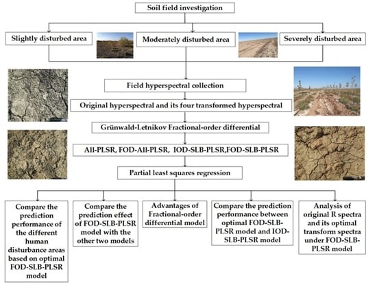
In this study, the hyperspectral reflectance of five kinds of spectra (R, , 1/R, lgR, 1/lgR) at different fractional orders were calculated by collecting the field hyperspectral data of soil samples from different human disturbance areas. Bands reaching a 0.01 significance level at different fractional orders were extracted to establish a significance level band partial least squares model (FOD-SLB-PLSR) based on the fractional-order differential. The purposes of this study were (1) to establish a soil salt content prediction FOD-SLB-PLSR model with high precision under different human disturbance conditions for the three areas, and to compare the results with those of PLSR models established by other methods (All-PLSR, FOD-All-PLSR, IOD-SLB-PLSR), (2) to conclude what kind of spectrum transformation data (R, , 1/R, lgR, 1/lgR) are the best for predicting different soil salt content in areas with slight, moderate, and severe human disturbance, (3) to identify the effect of different pretreatment methods on the accuracy of soil salt content prediction, and to extract more detailed information via fractional-order differential modeling, and (4) to select the optimal input variables from soil hyperspectral band, combination significance level band, and fractional-order differential modeling.
2. Materials and Methods
2.1. Overview of the Research Areas
The research areas are located in Fukang City of Changji Hui Autonomous Prefecture in Xinjiang Uygur Autonomous Region, in the margin of alluvial fan (87°44′E–88°46′E, 44°45′N–45°45′N) to the southeast of Xinjiang 102 Corps. Fukang is an important part of the economic belt on the north slope of Tianshan Mountain, about 50 km from Urumqi and about 90 km from Changji Hui Autonomous Prefecture. Fukang is one of the typical representatives of arid areas in Xinjiang, with a total land area of about 853,500 hm2, and is the main backbone of the agriculture- and animal husbandry-based economy. Fukang City possesses limestone, coal, mirabilite, oil, and other important mineral resources, as well as Tianshan Tianchi, desert ecosystems, Bogda Peak, Wuyun mosque, and other important tourism sites.
According to the specific conditions of the ground surface in the research areas, 5 sampling lines were arranged in Area A, with spacing between the sampling lines of about 500 m to 700 m, and 6 representative sampling points set on each sampling line. Area B was also divided into 5 sampling lines with spacing of about 400 m to 600 m, with 5 to 7 representative sampling points set on each sampling line. Area C consisted of two tracts of farms, with areas smaller than that of A or B, and six sampling lines arranged with spacing between sampling lines of about 200 m to 400 m. Five representative sampling points were set on each sampling line. In each area, samples were collected at 30 points for a total of 90 sample points for sample collecting, as shown in
Figure 1. In this way, a grid covering different sub-areas was formed across the entire research area, and the sampling points did not only reflect the soil property of each sub-area, but also controlled for distribution uniformity of sampling points in each area.
2.2. Classification of Research Areas with Different Disturbance Levels
The inevitable disturbance caused by human activity is mainly reflected in the different methods, intensity, and duration of human land use. Therefore, under the process of land development in arid areas, inevitable disturbances of different degrees caused by human activity will affect the ecological environment of the area and will induce changes to the original scheme of ground water and surface water causing spatial disequilibrium of water content. This ultimately results in changes to the salt content transfer rate and transport channels, aggravating the complexity of salt and water variation. One principal result of this process is a change in soil characteristics.
The desert and woodland soils to the northwest of Fukang City in Changji Hui Autonomous Prefecture, Xinjiang, which are affected by human activity to varying degrees and represent a variety of landscape and land use modes, are targeted for experimental study to elucidate the relationship between soil properties and intensity of human activity. The soil samples were divided into three areas based on intensity of human activity: a lightly disturbed area (Area A), a moderately disturbed area (Area B), and a severely disturbed area (Area C). The field environment of soil collection and soil crust of samples in Areas A, B, and C are shown in
Figure 1c–e. The locations of the three areas are near one another, and are only separated by natural ditches and man-made fences. Thus, conditions such as soil properties, sun exposure, atmospheric temperature, humidity, and waterfall are essentially the same. Namely, the environmental backgrounds of the soils in the three areas were kept constant.
The sampling area was divided into three types of soil areas according to the degree of human interference (
Figure 1). The specific environments of the three study areas are described as follows:
Slightly disturbed area (Area A): there is a water conveyance canal from south to north in the study area (marked in the pink of
Figure 1b). Its length is 15.30 km, depth is 5 m, upper width and lower width are 24 m and 6 m respectively [
26]. Area A is far away from human settlements due to the blockage of the water canal; humans only occasionally visit this area, and its topography basically maintains its original state, without destruction of the original component information in the soil, and without effect on the original vegetation. The vegetation coverage in this area is relatively high, generally about 30%. In some areas, there is a
Haloxylon ammodendron forest. The associated plants are mainly salt-tolerant vegetation, such as
Haloxylon ammodendron,
Kalidium foliatum,
Tamarix chinensis,
Salsola collina,
Reaumuria soongonic, etc. In addition, there are a large number of biological crusts on the soil surface of Area A, which are black and well developed.
Moderately disturbed area (Area B): Area B is located near the 102nd Corps in Fukang City, Xinjiang Uygur Autonomous Region. The soil in this area was cultivated in the 1950s and then abandoned. The daily activities of humans interfere with this area to a certain extent, which has led to certain changes in the vegetation and destroyed the original composition information in the soil. The ridges that were ploughed at that time still remain on the soil surface today; the width of the ridges is about 3 m, the distance between the ridges is about 0.4 m, and the depth of the furrows is about 0.3 m. The vegetation coverage in this area is relatively low, about 15%, mainly short shrubs such as Salsola collina or Reaumuria soongonic, accompanied by a small amount of saline vegetation such as Tamarix chinensis and Alhagi spaysifolia. In addition, there are some biological crusts on the surface of some soils in Area B; the degree of development of biological crusts is relatively poor compared with those in Area A.
Severely disturbed area (Area C): Area C is mainly composed of two artificial forest farms. All the soil was plowed and developed around 2015, which meant it was strongly disturbed by human activities. A large amount of artificial land reclamation has resulted in the removal of all the original vegetation on the surface, and the various soil attributes have been changed, among them, soil salinity, organic matter, nitrogen, phosphorus and potassium have changed greatly. The artificially planted trees are mainly elm trees. The average tree height in the woodland is about 2.5 m, the average crown width is about 0.5 m × 0.5 m, the row spacing in the woodland is about 3 m, and the plant spacing is about 1 m. Plastic hose drip irrigation is used in the woodland, and white salt can be seen on the soil surface. There are also few crusts on the soil surface in Area C.
2.3. Collection of Soil Sample Data
Soil samples were collected from 1 to 10 October 2017, for 10 days in total, and were sampled according to the position information of the 90 sampling points set up in
Figure 1. We collected 5 topsoil samples from 0–10 cm depth within 1 m around each sampling point by using the plum-blossom pile sampling method. We thoroughly mixed the samples and place them in sealed sampling bags in an aluminum box, then sealed and marked the samples. Meanwhile, coordinate data of sampling points were recorded using GPS positioning, as well as the vegetation type, vegetation coverage, crusting condition, and land utilization. We also took photographs of the sampling environment at each sampling point. All soil samples were transported back to the laboratory, and after natural air-drying, impurity removal, grinding and sieving, were sent to the Xinjiang Institute of Ecology and Geography at the Chinese Academy of Sciences for determination of total salt content.
2.4. Measurement of Soil Hyperspectral Data
The field hyperspectral data of the soil samples were measured using a FieldSpec®3Hi-Res type ground-object spectrometer manufactured by American ASD (Analytical spectral device). The measurements range of all bands was 350–2500 nm, and the number of output bands was 2151, in which the band range of 350–1000 nm was visible light with a spectral resolution of 3 nm and a sampling interval of 1.4 nm. The band range of 1001–2500 nm was near infrared with a spectral resolution of 8 nm and a sampling interval of 1.1 nm. The resampling interval was 1 nm.
The collection of field soil and soil sample hyperspectral data were performed at the same time, from 12:30–15:30 local time, and the measurements were conducted when weather conditions were clear, sunny, and not windy. The FieldSpec
®3Hi-Res ground-object spectrometer was subjected to a whiteboard correction operation prior to each soil hyperspectral collection, and the soil was measured only when 100% of the baseline was obtained [
26,
27]. Measurements were taken at 25 °C of the probe field view angle and at a height of 15 cm vertical to the ground, during which 5 points were chosen within 1 m of each sample point. Measurements were replicated 10 times at each point, thus 50 hyperspectral data readings were collected from each sample point. The average value of 50 hyperspectral data readings was calculated using View Spec Pro software pre-sets in the spectrometer, which was then taken as the measured hyperspectral reflectance value of each sample point. In addition, researchers made careful observations upon each hyperspectral data measurement. If any outlier hyperspectral data were measured, the data were excluded from analysis and soil was measured again.
2.5. Delete Interference Bands
The soil hyperspectral reflectance data measured by the FieldSpec
®3Hi-Res spectrometer has a detection band range of 350–2500 nm, and each hyperspectral reflectance data reading contains 2151 bands’ information. However, the ultraviolet bands for 350–399 nm and the short-wave infrared bands for 2401–2500 nm collected by the spectrometer are affected by noise, which results in a low signal-to-noise ratio, large amplitude changes, poor data quality, and data instability. This paper takes the 23rd soil sample in Area A as an example: the hyperspectral reflectance of the edge bands is shown in
Figure 2, and the fluctuation of the hyperspectral reflectance is relatively large. Therefore, this paper deletes the 350–399 nm and 2401–2500 nm edge bands.
Figure 3,
Figure 4 and
Figure 5 show the original hyperspectral reflectance values of soils in Areas A, B, and C at 350–2500 nm, and the original hyperspectral reflectance of the three regions fluctuates very obviously in the 1350 nm and 1900 nm bands, which was caused by the influence of the soil moisture absorption bands. At the same time, when we collect field hyperspectral data, those bands will have a greater impact on the accuracy of the quantitative prediction model for soil total salt. Therefore, this study deletes the 1340–1420 nm and 1800–1960 nm bands located near the moisture absorption bands, and deletes the 350–399 nm and 2401–2500 nm bands.
Figure 3b,
Figure 4b and
Figure 5b show the hyperspectral reflectance curves with deletion of the interference bands. There was a total of 1759 bands remaining when the interference bands were deleted.
2.6. Grünwald-Letnikov Fractional-Order Differential
In 1867, the mathematician Grünwald first proposed an analytical fractional-order differential formula using the Gamma and Mittag–Leffler functions. However, the mathematician Letnikov, who was completely unaware of the definition of Grünwald’s work, independently derived another expression using the same method in 1868. Such is the present definition of Grünwald–Letnikov, which extends the order range of the classical integral differential with continuous functions [
28] from the integral order to the fractional order by calculating the limit of the difference approximate recursion formula of the original integral differential [
29,
30,
31].
Since Grünwald–Letnikov’s is a discrete definition, it is convenient for numerical calculation. Thus, in this study, we use the Grünwald–Letnikov expression to research hyperspectral signals. The formula is as follows:
where p represents the order of the differential, the p order differential when p is a positive real number, and the p order integral when p is a negative real number. h represents the differential step, t represents the upper limit of the differential, a represents the lower limit of the differential, and
represents the Gamma function.
The derivation of Equation (1) is as follows:
Assuming an
order differential in the function f(x), then the first order differential f(x) is defined as:
The second order differential of
is defined as:
The third order differential of
is defined as:
By analogy, the n
th order differential of the function
can be deduced by mathematical induction as:
In which, represents the number of combinations,
Since the binomial expansion can be expressed as Equation (6):
The coefficients of the binomial can be directly calculated by Equation (7):
By extending the formula for calculating the n-order differential to the case of non-integer v, the expression of the binomial can be changed into the form of infinite series, namely:
Then the expression of the extended binomial can be expressed as Equation (9):
Assuming , the value of the function f(x) is zero and the sum of infinite terms can be transformed into the sum of finite terms. Thus, expression of the Grünwald–Letnikov fractional-order differential derived at this time is shown in Equation (1).
Assuming that the function f(x) is a one-dimensional hyperspectral signal, the band range is
,
equally divided by the differential step
. Since the resampling interval of the ASDFieldSpec
®3Hi-Res spectrometer is 1 nm, the differential step can be set as
. Thus, the difference expression of the v order fractional-order differential of the function f(x) can be derived from Equation (1) as follows:
In Equation (10), represents 0.0 order differential; that is, no fractional-order differential processing is performed on the hyperspectral. represents a 1.0 order differential of the integral order, and represents a 2.0 order differential of the integral order. In this study, the fractional-order differential pre-processing calculation on the hyperspectral signal is performed using Matlab software.
From Equation (10), the v-order fractional-order differential value of function f(x) in the given band is related not only to the hyperspectral reflectance f(x) of the band, but also the hyperspectral reflectance of all bands prior. That is, the reflectance is related to , , , , . Moreover, the calculation process incorporates point distance as a parameter affecting the value of the fractional-order differential. That is, the weight value corresponding to closer points is larger and the influence on the differential value is likewise greater, while the weight value corresponding to farther points is smaller and the influence on the differential value is likewise smaller. This property reflects “memory” and “global” in the fractional-order differential, which is the most significant difference between fractional and integral differential.
2.7. Modeling Process of FOD-SLB-PLSR Model
We sorted bands reaching a 0.01 significance level band (i.e., the characteristic band) of each spectral transformation for total salts at different differential orders, then took the corresponding hyperspectral reflectance thereof as an independent variable. Data on the total salts were treated as dependent variables to establish the partial least squares regression (FOD-SLB-PLSR) model based on the significance level bands of fractional-order differential (realized on Matlab software). The modeling steps used are as follows:
① Carry out four mathematical transformations (, 1/R, lgR, 1/lgR) on the original soil hyperspectral data (R) to obtain various transformed hyperspectral data.
② Calculate the correlation coefficient between the original spectrum of 0.0-order (0.0-order indicates no performed differential value calculation) as well as its transformed data and total salt, then test the significance level of the correlation coefficient. Select the band for which the test result reaches the 0.01 significance level as the characteristic band of the differential order. If no correlation coefficient of any band at the order of 0.0 passes the 0.01 significance test, then carry out step ④.
③ Take the hyperspectral reflectance corresponding to the selected characteristic band from step ② as the independent variable, and the salt data as the dependent variable, then use the partial least squares regression method to build the model.
④ Execute the calculation if order of differential , then continue to execute step ⑤. Otherwise, continue to execute step ⑦.
⑤ Take 0.1 as the order interval of the fractional-order differential, then use formula (10) from
Section 2.5 to calculate the spectral data of the original spectrum and its transformed data following the 0.1 order differential.
⑥ Repeat steps ② to ⑤ until orders 0.0–2.0 have been completed.
⑦ End of modeling process.
The FOD-SLB-PLSR model building process is as shown in
Figure 6.
2.8. Evaluation Method of Model Precision
In this paper, five precision evaluation indices are used to evaluate the effect of prediction modeling [
32,
33]. That is, the coefficient of determination for calibration dataset (
), root mean squared error for calibration dataset (
), coefficient of determination for validation dataset (
), root mean squared error for validation dataset (
), and the ratio of the performance to deviation (RPD) of the model. The calculation formulas of
, RMSE, and PRD are as follows [
34,
35,
36]:
where n represents the number of soil samples;
represents the measured values of the ith soil sample;
represents the average of the measured values of all soil samples;
represents the predicted values of the ith soil sample;
represents the average of the predicted values of all soil samples; and SD represents the standard deviation of the soil sample in the validation dataset.
In general, the optimal prediction model has the largest
and RPD values and the smallest RMSE value.
indicates the degree of fit and stability of the model. The closer its value to 1, the higher the degree of fit and the better the stability of the model. When
, the fit between the predicted value and measured value of the model and stability were excellent. When
, the fit between the predicted and measured values of the model was very good, as well as the stability. When
, the fit between the predicted and measured values was acceptable, and the stability was relatively good. The smaller and closer to 0 the value of RMSE, the smaller the prediction error of the model and the higher the prediction accuracy. RPD is used to evaluate the ratio of the performance to deviation of the prediction model [
37,
38,
39]. When
, the prediction capability of the model was excellent. When
, the prediction capability of the model was very good. When
, the prediction capability of the model was relatively good. When
, the prediction capability of the model was average. When
, the prediction capability of the model was poor. When
, the prediction capability of the model was very poor and a prediction could not be made.
The dataset needed to be divided into validation and calibration datasets before establishing a hyperspectral prediction model. The concentration gradient method was used as the basis for classification, which selects the samples as the validation dataset samples according to a certain concentration interval of all the soil samples based on the total salt content. This method can ensure that the selected validation dataset sample data is relatively evenly distributed in all soil sample data, so the selected sample has a certain degree of representativeness. A total of 90 soil samples were collected in this study, and 30 samples were in Areas A, B, and C respectively. The dataset was divided by the concentration gradient method. Therefore, 20 samples were selected as the calibration dataset, and 10 samples were selected as the validation dataset.
3. Simulation Results
The estimation results of All-PSLR, FOD-All-PLSR, and FOD-SLB-PLSR models on total salt in each area were all sorted out to clearly explain the difference of total salt prediction in different areas by different methods. The estimation results of the soil total salt in Areas A, B, and C are shown in
Table 1,
Table 2 and
Table 3, respectively.
The All-PSLR model takes the hyperspectral reflectance corresponding to all bands as the independent variable. The PLSR model based on the five spectra had very poor predictive ability, and its RPD value was less than 0.5 in Areas A and C, and less than 1 in Area B, meaning that the total salt content of three regions could not be predicted.
The FOD-All-PLSR model is a method based on the All-PSLR model, which uses the hyperspectral reflectance of all bands after fractional differentiation as an independent variable to establish a PLSR model. Compared with the All-PSLR model, its prediction effect was improved to some extent, but the improvement was still not large. Its RPD value was less than 1 in the three regions, and it was still unable to effectively predict the total salt in the three regions.
While the FOD-SLB-PLSR model showed improvement over the FOD-All-PLSR model that is, taking the significance band reaching 0.01 level as the characteristic band after fractional-order differential to establish the PLSR model, it eliminated the band variables with low correlation and obtained an estimation model with good prediction and high stability. Compared with the All-PSLR and FOD-All-PLSR model, the prediction of this model was improved greatly.
3.1. Area A
3.1.1. Prediction of Total Salt Content in Area A by Different Estimation Models
There were four models (R of order 1.4, R of order 1.8, 1/lgR of order 1.6, and
of order 1.8) in the FOD-SLB-PLSR model with RPD values between 1.8 and 2.0 (
Figure 7), and the R
2 values were between 0.66 and 0.80. This shows that the four models had good ability to predict soil total salt content in Area A, and the fitting effect between predicted and measured values was also good. Among them, RPD, R
2, and RMSE of the validation dataset were 1.8126, 0.7608, and 3.6691, respectively in the R model of order 1.4. Similarly, these values were 1.8715, 0.7199, and 3.4859, respectively in the R model of order 1.8; 1.8444, 0.6759, and 3.2087, respectively in the
model of order 1.8; and 1.9061, 0.7121, and 3.2268, respectively in the 1/lgR model of order 1.6. Thus, the optimal model for predicting the total salt content in Area A was the 1.6 order 1/lgR, in which the RPD was enhanced by 1.85%, R
c2 was enhanced by 4.58%, and RMSE
v and RMSE
c were reduced by 7.43% and 90.44%, respectively, compared to the optimal 1.8 order fractional model of the original spectrum.
From the above analysis, the optimal FOD-SLB-PLSR model was superior not only to All-PSLR models, but also to all FOD-All-PLSR models (
Table 1). That is to say, the fractional-order differential model reaching 0.01 level significance test band can eliminate the redundancy, fully extract hyperspectral information, and model to predict soil salt information well. Meanwhile, in the FOD-SLB-PLSR models, good prediction was seen among higher-order differentials (above 1.4 order), and the RPD of optimal FOD-SLB-PLSR model was enhanced by 1.85% compared with the optimal R-based FOD-SLB-PLSR model (fractional order 1.8).
Meanwhile, the optimal prediction model for each method was selected for easier comparison. Among them, All-PLSR represented a PLSR model based on all bands, and only the prediction results of R and the optimal transformation at the order of 0.0 (i.e., when no differential value calculation was performed) are listed. FOD-All-PLSR represents the PLSR model based on all bands of the fractional-order differential, and only prediction results of R and the optimal transformation at the optimal differential order are listed. FOD-SLB-PLSR represents the PLSR model based on the 0.01 significance level bands of the fractional-order differential, and only the prediction results at the optimal differential order of each of the five spectra are listed below.
3.1.2. Scatter Plots of Prediction Models
The sample data of the validation dataset was used for testing in order to verify the prediction accuracy of the total salt for the estimation model with five spectra (
Figure 8). The black dotted line represents the 1:1 regression line, and the blue solid line represents the fitted equation line between the predicted value and the measured value. When the fitting equation line is closer to the 1:1 regression line, it indicates that the prediction accuracy of the model is higher. The data points in the All-PSLR and FOD-All-PLSR models are very scattered on both sides of the fitted line.
It can be seen from
Figure 8 showing the FOD-SLB-PLSR model that the measured and predicted data of the 1.6-order 1/lgR, 1.8-order
, and 1.8-order R models are more evenly distributed on both sides of the fitting line. The fitting degrees of these three models are better. However, the prediction effect based on the 1.6-order 1/lgR model is the best: the maximum RPD is 1.9061, the smaller RMSE is 3.2268, the larger R
2 is 0.7121, and the fitting equation is expressed as
.
3.2. Area B
3.2.1. Estimation of Total Salt Content in Area B by Each Modeling Method
The RPD values of two models (1/R of order 1.7 and 1/R of order 1.9) in the FOD-SLB-PLSR model were greater than those calculated with 1.8 (
Figure 9), and R
2 values were between 0.66 and 0.80, indicating that the predicted and measured values of these two models fitted well. Of these, the RPD, R
2, and RMSE of the verification dataset were 1.8315, 0.6876, and 6.5592, respectively in the 1.9-order 1/ R model; and 2.0761, 0.7458, and 6.9361, respectively in the 1.7-order 1/R model. This indicates that the 1/R model of order 1.9 had a good prediction ability for total salt content. The 1.7-order 1/R model was the optimal model for predicting soil total salt content in Area B, and prediction results showed an improvement in RPD by 19.06% and in R
v2 by 5.56% with a reduction in RMSE
v by 40.23% compared with the optimal 1.6-order fractional model of the original spectrum.
In summary, we see that the optimal model for predicting total salt content in Area B was the optimal FOD-SLB-PLSR model, and a few models with relatively good predicting ability were mainly concentrated in the fractional orders of 1.7 and 1.9 of 1/R. The fractional differentiation of 1/R can eliminate the noise of soil spectral reflectance in areas with moderate disturbance. Furthermore, the RPD in the optimal FOD-SLB-PLSR model was enhanced by 19.06% compared with the optimal fractional 1.6-order of FOD-SLB-PLSR model based on R.
3.2.2. Scatter Plots of Prediction Models
The accuracy of the prediction model to estimate the total salt with the validation dataset data is shown in
Figure 10. The data points in the All-PSLR and FOD-All-PLSR models are scattered and not distributed around the fitted line.
It can be seen from
Figure 10 showing the FOD-SLB-PLSR model that the data points of the 1.7-order 1/R model are very evenly distributed on both sides of the fitting line, and the fitting equation is
. The RPD, R
2, and RMSE values of the validation dataset are 2.0761, 0.7458, and 6.9361, respectively. Moreover, the data points of the 1.6-order R, 1.9-order
, and 1.6-order lgR models are also relatively evenly distributed on both sides of the fitting line, but the fitting effect is not as good as that of the 1.7-order 1/R model.
3.3. Area C
3.3.1. Prediction of Total Salt Content in Area C by Various Methods
The RPD values of FOD-SLB-PLSR model in two models (lgR of order 1.8 and lgR of order 1.9) were between 2.0 and 2.5 (
Figure 11) and R
2 values were between 0.75 and 0.85. Among these values, the RPD, R
2, and RMSE for the verification dataset were 2.2892, 0.8202, and 6.6363, respectively, under the 1.8-order lgR model; and 2.1370, 0.7996, and 5.3727, respectively, under the 1.9-order lgR model. Therefore, the lgR of order 1.9 shows a good prediction strength for total salt content, and the fitting effect between predicted values and measured values was favorable. The 1.8-order lgR model is the optimal model for predicting soil total salt content in Area C and has a good prediction strength for total salt content. The fit between predicted and measured values was also good. Compared with the optimal 1.8-order fractional model of the original spectrum, RPD was enhanced by 46.23%, R
v2 was enhanced by 45.92%, and R
c2 was enhanced by 23.63%, while RMSEv and RMSE
c were reduced by 25.05% and 31.09%, respectively.
It can be concluded that under FOD-SLB-PLSR models, a few models with good prediction ability were concentrated near the fractional orders of 1.8 and 1.9 for lgR. This indicates that estimation of soil total salt content in areas with severe human disturbance not only requires the original data’s spectral transformation (especially the logarithmic transformation), but also fractional-order differential processing. If these conditions are satisfied, the model can estimate the total salt content in Area C. Furthermore, compared with the optimal FOD-SLB-PLSR model (1.8 order) based on R, the optimal FOD-SLB-PLSR model RPD values were enhanced by 46.23%.
3.3.2. Scatter Plots of Prediction Models
The test results of the prediction model to estimate the total salt are shown in
Figure 12. The data points in the All-PSLR and FOD-All-PLSR models are very scattered on both sides of the fitted line.
The test results of the optimal FOD-SLB-PLSR model for
Figure 12(c1–c5) show that the data points of the 1.8-order lgR model are most evenly distributed around the fitting line, and the RPD, R
2, and RMSE of the validation dataset are 2.2892, 0.8202, 6.6363, respectively. The fitting equation is
, so this model has the best prediction effect on the total salt in Area C. The 1.2-order 1/lgR model has the worst test effect, and the data points are very scattered on both sides of the fitted line. The data points of the 1.8-order R and
models are also scattered around the fitting line. The data points of the 1.0-order 1/R model are relatively evenly distributed around the fitting line.
4. Discussion
4.1. Compare the Prediction Performance of the Different Human Disturbance Areas Based on Optimal FOD-SLB-PLSR Model
The disturbance of the ecosystem has become a widespread phenomenon. In the arid and semi-arid areas of China, because there is interference such as human grazing and agricultural activities, humans have reclaimed large areas of wasteland into cultivated land and forest land. However, few scientists have compared and analyzed the prediction performance of soil salinity models in different human interference environments. Duan et al. [
26] adopted a multiple linear regression model to predict the salt content of the three interference regions, but did not use the preprocessing method of fractional-order differential modeling. Tian et al. [
40] employed a multiple regression model to quantitatively estimate soil total potassium content in one region, and did not compare the estimation effect of different research areas. Fu et al. [
41] only studied the pretreatment effect of soil total phosphorus content in one region, but did not analyze the prediction performance. Moreover, this paper compares the prediction effects of total soil salt models in different interference regions in detail. The results of the proposed FOD-SLB-PLSR model vary greatly on the prediction of total salt content in different human disturbance areas, which can be seen from
Table 1,
Table 2 and
Table 3.
In the area with slight human activity, the FOD-SLB-PLSR model based on the 1/lgR transform spectrum of 1.6-order was the best model for predicting the total soil salt in Area A, and its RPD, R2, and RMSM were 1.9061, 0.7121, 3.2268, respectively. The prediction effect based on the R original spectrum of 1.8-order for RPD, R2, and RMSM were 1.8715, 0.7199, 3.4859, respectively. Those results indicate that the prediction accuracy of the soil total salt content model based on the original spectral data preprocessed by fractional-order differential modeling is almost the same as that of the optimal model based on the 1/lgR transformed spectral preprocessed by fractional-order differential modeling.
In the area of moderate human activity, the optimal model for predicting soil total salt content was based on the 1/R transformation of the original spectrum then processed by fractional-order differential modeling. This best model was the 1/R transform spectrum of 1.7-order, and its RPD, R2, and RMSM were 2.0761, 0.7458, 6.9361, respectively. It shows that the prediction capability of the best model was very good.
In the area with severe human activity, the model based on lgR transformation through 1.8-order fractional-order differential pretreatment was best; its RPD, R2, and RMSM were 2.2892, 0.8202, 6.6363, respectively, and its prediction capability was very good due to its RPD value between 2.0 and 2.5.
These results may indicate that the greater the degree of disturbance to the soil, the greater the need to transform the original spectrum. Meanwhile, the RPD values that provided an optimal FOD-SLB-PLSR model for each area were: Area A (1.9061) < Area B (2.0761) < Area C (2.2892). This indicates that the prediction effect of data processed by fractional-order differential calculation increases with human disturbance increases and results in a higher-precision model.
4.2. Compare the Prediction Effect of FOD-SLB-PLSR Model with the Other Two Models
The results of
Table 1,
Table 2 and
Table 3 show that the prediction performance of the optimal FOD-SLB-PLSR model for each area was superior to corresponding All-PSLR, and FOD-All-PLSR models for soil total salt content. It indicates that the original soil hyperspectral data undergo spectral transformation and fractional-order differential processing is insufficient. This is because a total of 1759 all band variables were included in the All-PSLR and FOD-All-PLSR models, and there were a large number of redundant band variables, which will not only lead to low accuracy of the prediction model, but also make the calculation of the model large. Therefore, it was necessary to further select the characteristic band information. This paper chose the characteristic band based on the 0.01 significance level band (SLB). The PLSR model established based on the characteristic waveband not only reduced the calculation required of the model, but also improved the prediction accuracy of the model.
Therefore, in order to achieve a good or relatively good prediction ability for these models, it is necessary to carry out fractional-order differential processing and use a model with bands that achieve a 0.01 significance level test. The method of extracting feature bands based on the significance level in this paper is consistent with previous research results of scientists. For example, Chen et al. [
42] estimated the nitrogen concentration of rubber trees using fractional calculus, and the PLSR was utilized to develop the estimation models with the wavelengths selected by significant test of correlation coefficient at 0.01 level. Zhang et al. [
43] studied the quantitative estimation of salt content of saline soil, and bands whose correlation coefficient passed the significance test at the level of 0.01 were used as features to participate in the modeling process.
4.3. Compare the Prediction Performance between Optimal FOD-SLB-PLSR Model and IOD-SLB-PLSR Model
IOD-SLB-PLSR represents a PLSR model based on significance level bands of integral differentials (1.0 and 2.0). The results of the optimal FOD-SLB-PLSR model compared with the optimal IOD-SLB-PLSR model are shown in
Table 4.
In Area A, compared with the model based on 1.0-order 1/lgR in prediction performance of the total salt content, the RPD of the optimal FOD-SLB-PLSR model was enhanced by 9.83%, R
c2 was enhanced by 0.38%, and RMSE
v and RMSE
c were reduced by 27.83% and 40.76%, respectively. Compared with the model based on 2.0-order 1/R, the RPD of the optimal FOD-SLB-PLSR model was improved by 21.91%, R
v2 was improved by 22.63%, and R
c2 was improved by 3.62%, while RMSE
v and RMSE
c were reduced by 29.90% and 89.96%, respectively (
Table 4). Furthermore, compared with the best integral order differential model (IOD-SLB-PLSR of 1.0-order 1/lgR), the RPD of the optimal FOD-SLB-PLSR model was enhanced by more than 9%.
In Area B, compared with the IOD-SLB-PLSR model based on 1.0-order 1/lgR prediction, the optimal FOD-SLB-PLSR model had a 59.26% improvement in RPD, 106.76% improvement in Rv2, 8.90% in Rc2, and a 51.69% reduction in RMSEv and 22.01% reduction in RMSEc. Compared with the IOD-SLB-PLSR model based on R of 2.0-order, the RPD of the optimal FOD-SLB-PLSR model improved by 45.66%, Rv2 improved by 59.50%, and RMSEv was reduced by 35.37%. Furthermore, compared with the optimal IOD-SLB-PLSR model (2.0-order R), the RPD in the optimal FOD-SLB-PLSR model was enhanced by more than 45%.
In Area C, compared with the 1/R of 1.0-order under the IOD-SLB-PLSR model in prediction performance of total salt content, the optimal FOD-SLB-PLSR model showed a 22.61% improvement in RPD, 4.98% improvement in Rv2, and 1.92% improvement in Rc2, while a 23.87% reduction was seen in RMSEv and a 5.06% reduction was seen in RMSEc. Compared with the lgR of 2.0-order under the IOD-SLB-PLSR model, RPD was enhanced by 51.17%, Rv2 was enhanced by 46.75%, and RMSEv was reduced by 15.25%. Furthermore, compared with the best integral differential model (IOD-SLB-PLSR), the optimal FOD-SLB-PLSR model RPD values were enhanced by more than 22%.
The optimal model was revealed in the fractional order results instead of the integer order results in the three regions, which is consistent with previous research results of scientists. For example, Wang et al. [
44] combined fractional-order differential and PLSR models to predict the organic matter content; the optimal model also was revealed in the fractional order of 1.8. Hong et al. [
23] used the partial least square–support vector machine (PLS–SVM) model to estimate the soil organic matter content, and the 1.25-order derivative spectra exhibited the best model performance. Zhang et al. [
25] found the 1.05- to 1.45-order range of PLS–SVM had the highest signal-to-noise ratio and was most suitable for soil organic matter content analysis.
4.4. Advantages of Fractional-Order Differential Model
Figure 13 shows the number of bands where the correlation coefficients between the five spectra and total salt passed the 0.01 significance level test. When the fractional order in Area A was from 0.0-order to 0.5-order, in Area B is from 0.0-order to 0.4-order, and in Area C from 0.0-order to 0.2-order, none of the correlation coefficients of any bands passed the 0.01 significance level test. It can be seen that the number of bands that passed the 0.01 significance level test in the fractional order was obviously more than those in the integer order, and these bands were concentrated in the high-order fractional order. For example, they were mostly around the 1.2-order in the slight human interference region, around the 1.8-order in the moderate interference region, and around the 1.3-order in the severe interference region.
The FOD-SLB-PLSR models with optimal prediction ability were all concentrated at the higher order differential. The results of this paper are basically consistent with those of previous scientists. For instance, Lao et al. [
45] found that the optimal fractional-order differential spectra of Ca
2+, CO
32− and Cl
− were on the 1.65-, 1.90-, and 1.55-order derivative spectra, respectively. Xu et al. [
46] found that the optimal performance was achieved by the 1.8-order, 1.6-order, and 1.2-order spectra for Hg, Cr, and Cu, correspondingly. Wang et al. [
47] found the most effective model was established based on random forest with the 1.5-order derivative.
4.5. Analysis of Original R Spectra and Its Optimal Transform Spectra under FOD-SLB-PLSR Model
No matter which spectrum transformation was used under the FOD-SLB-PLSR model, the fractional-order differential order of the optimal model was often similar to that of the optimal model based on the fractional-order differential of the original spectrum (
Table 5). For instance, the fractional-order differential order of optimal model was the 1.6-order based on the1/lgR transform spectrum in Area A, while it was the 1.8-order based on the R spectrum. In addition, it was the 1.7-order of optimal model based on the 1/R transform spectrum in Area B, while it was the 1.6-order based on the R spectrum. Moreover, it was the 1.8-order of the R spectrum and the optimal lgR transform spectrum in Area C. This suggests that the order of the optimal model of the fractional-order differential is closely related to its optimal model for the original spectral differential.


 ,
, 


